A New VSLMS Algorithm for Performance Analysis of Self Adaptive Equalizers

International Journal of Trend in Scientific Research and Development (IJTSRD)

Volume 5 Issue 1, November-December 2020 Available Online: www.ijtsrd.com e-ISSN: 2456 – 6470

A New VSLMS Algorithm for Performance

Analysis of Self Adaptive Equalizers

B. R. Kavitha

_{, P. T. Jamuna Devi}

1

_{Assistant Professor, Department of Computer Science,}

Vivekanandha College of Arts and Sciences for Women, Tiruchengode, Tamil Nadu, India

2

_{Online Content Developer, Worldwide Teacher Academy,}

A Unit of My Canvas Private Limited,

Coimbatore, Tamil Nadu, India

The fundamental feature of the LMS (Least Mean Squares) algorithm is the step size, and it involvesa cautious adjustment. Large step size may lead to loss of stability which are required for fast adaptation. Small step size leads to low convergence which are needed for insignificant excess mean square error. Consequently, several changes of the LMS algorithm in which the step size modifications are made throughout the adaptation method which depend on certain specific features, were and are still under development. A new variable step-size LMS algorithm is examined to solve the problem of LMS algorithm. The algorithm will be based on the sigmoid function which develops the non-linear functional relation among error and step. The algorithm solves the problem of setting parameters in the function by introducing the error feedback strategy to adjust the parameters adaptively. Compared with other algorithms, simulation results show that the algorithm performs perfect at convergence rate and steady-state error with a better applicability.

KEYWORDS: Inter symbol interference, Least Mean Square, Bit Error Rate, Adaptive Equalizer, communication channel, Evolutionary Programming

How to cite this paper: B. R. Kavitha | P. T. Jamuna Devi "A New VSLMS Algorithm for Performance Analysis of Self Adaptive Equalizers" Published in International Journal of Trend in Scientific Research and Development (ijtsrd), ISSN: 2456-6470, Volume-5 | Issue-1, December 2020, pp.1517-1523, URL: www.ijtsrd.com/papers/ijtsrd38229.pdf Copyright © 2020 by author (s) and International Journal of Trend in Scientific Research and Development Journal. This is an Open Access article distributed under the terms of

the Creative

Commons Attribution

License (CC BY 4.0)

(http://creativecommons.org/licenses/by/4.0)

1. INTRODUCTION

The algorithm of LMS (Least mean square)[1] is widely used in many areas as radar system due to its simpleness. LMS algorithm is based on the steepest descent principle; it replaced the random grad by instant grad and reach at the optimized weight along the negative direction of weight grad to minimize the mean square error. But the requirement for the convergence rate and the steady state error by LMS algorithm with the fixed step size is contradictory. Reference [2] presented the algorithm that variable step-size parameter is proportional to the error, as improves the performance, but not ideal. Reference [3] presented a method called S function variable step-size LMS algorithm (SVLMS), step adjustment strategy of the algorithm is advanced to some extent, but the step changes sharply when the algorithm error approximate zero, as may increase the steady-state error. Reference [4] made further improvement on the basis of reference [3], and corrected the step sharp changes when the algorithm error approximate zero, but the key parameters in the algorithms need to set manually, and the improper parameter setting will seriously affect the performance of the proposed algorithm. Reference [5-6] presented the relevant variable step-size LMS algorithm respectively based on versiera, hyperbolic tangent function and arc tan function to remit the contradiction between convergence rate and steady-state error partly. This paper presents the Error Feedback Least Mean Square (VSLMS)

algorithm based on Sigmoid function referring to Reference [4].The algorithm uses the feedback idea by introducing the parameter error factor to solve problems on Sigmoid parameter setting, it can improve the convergence rate, steady-state error and other performance indexes, and it has the extensive adaptability.

Generally utilized filters can be split into three types: adaptive filter, IIR (Infinite Impulse Response) filter, and FIR (Finite Impulse Response) filter. FIR filter can be intended as the system with linear phase characteristic and random amplitude-frequency characteristic. The planning objective of FIR filter is that the necessary condition of filter coefficients for performing indexes should be satisfied and the hardware resources of system could be saved. Contrasting with FIR filter, IIR filter has greater effectiveness and lower order in accordance with condition of similar amplitude-frequency response. Though, the drawback of IIR filter is the non-linear stage characteristic, which limits the implementation range of filter. In this article, the hypothetical basis of IIR filter and FIR filter is the Linear Time-Invariant System, which implies analysis method and the structure design among IIR filter and FIR filter are comparable. In a word, FIR filter is appropriate to the condition that the amplitude-frequency characteristic is various from the linear phase characteristic or the

conventional filter characteristic is necessary; IIR filter is appropriate to the requirement that the amplitude-frequency characteristic is provided and the phase characteristic is not taken into account.

2. ADAPTIVE FILTER OF THE CLOSED-LOOP SYSTEM

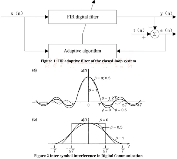
In this article, the structure factors of the adaptive filter analyzed could be automatically adjust by the usage of LMS algorithm, in accordance with the numerical characteristics of input signal. The adaptive filter is comprised of the digital filter with adaptive algorithm and adjustable factors. This article concentrates on the FIR adaptive filter of the closed-loop system, which is demonstrated in Figure 1. A y(n) is the output signal which is being generated with the usage of FIR digital filter and is associated with the input signal x(n). A e(n) is the error signal which is generated with the contrast

of target signal t(n) an output signal y(n). The filter factors can be altered routinely, in accordance with the optimum standard for error signal an FIR adaptive filter. The method of adjusting factors of FIR adaptive filter is referred to as the “tracking process” once the statistical features of input signals are undetermined and the procedure of adjusting factors of FIR adaptive filter is referred to as the “learning process” once the statistical features of input signals are being analyzed. An adaptive filter is primarily comprised of the digital filter with the adaptive algorithm and the adjustable factors. The final aim of adaptive algorithm is to encounter the optimum measure of error expected signal, and among estimated signal and the optimum algorithm is the determining factor for the structure and performance of adaptive measure. This article approves LMS algorithm as the optimum benchmark to solve the optimum problem.

Figure 1: FIR adaptive filter of the closed-loop system

Figure 2 Inter symbol Interference in Digital Communication

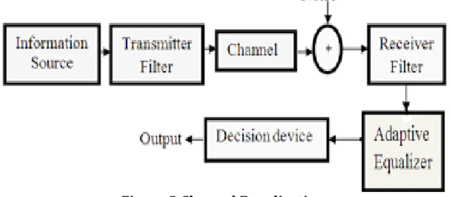
3. NECESSARY FOR CHANNEL EQUALIZATION

Adaptive equalizers may be unsupervised and supervised equalizers. In supervised equalizers it is required to stimulate the system on a regular basis with a recognized training or experimental signal disrupting the broadcasting of practical information. A reproduction of this experimental signal is also available at the transmitter and the transmitter relates the response of the entire system with input to automatically update its factors. Various communication systems such as digital radios or digital television do not offer the range for the usage of a training signal. In such a condition the equalizer requires some form of self-recovery or unsupervised technique to update its factors are referred to as blind equalizers. Latest developments in signal processing methods have offered broad range of nonlinear equalizers. In nonlinear channels with the period for differing attributes, nonlinear equalizer offers improved performance in comparison to linear equalizers due to their nonlinear determination made by the boundaries.

Figure 3 Channel Equalization

Figure 3 demonstrates the usage of adaptive equalizer for channel equalization in a communications system. The knowledge of the ‘desired’ response was required by an adaptive filtering algorithm to form the error signal necessary for the adaptive procedure in order to operate. For the adaptive equalization, the communicated series is the ‘desired’ response. In practice, an adaptive equalizer is situated at the transmitter and is actually split from the source of its perfect desired response. One technique to generate the required response locally in the receiver is the usage of training order in which a reproduction of the desired response is stored within the receiver. Obviously, the power generator of this stored reference must be electronically synchronized with the known transmitted sequence. Second method is decision directed technique in which a great facsimile of the communicated series is being generated at the output of the decision device in the receiver. If this output is accurate communicated series, then it is utilized as the ‘desired’ response for the rationale of adaptive equalization.

3.1. Inter symbol Interference in Digital Communication

Several channels for communication, containing several broadcasting channels and telephone channels, may be commonly described as a band-limited linear filters. Subsequently, this type of channels is termed by their response of frequency C (f), which could be stated as

(1)

where, ϕ( f ) is referred to as the phase response and A(f) is referred to as the amplitude response. An additional feature thatis occasionally utilized in the location of the phase response is the group delay or envelope delay, which has been characterized as

(2)

A channel is believed to be ideal or non-distorting if, within the bandwidth Minhabited by the communicated signal, ϕ( f ) is a linear function of frequency and A( f ) =constant [or the envelope delay τ( f ) =constant]. Instead, if τ( f ) and A( f ) are not constant within the bandwidth inhabited by the transferred signal, the signal is distorted by the channel. If τ( f ) is not constant, a distortion on the transferred signal is referred to as delay bias and if A( f ) is not constant, the deformation is referred to as amplitude distortion.

As a consequence of the delay distortion and amplitude resulting from then on-ideal channel frequency response feature C(f ) , a sequence of pulses broadcasted through the channel at rates comparable to the bandwidth M are denigrated to the point that they will no longer be noticeable as well-characterized pulses at the collecting terminal. On the other hand, they correspond and, consequently, we have ISI (Inter symbol interference). As an instance of the impact of 2 delay distortion on a transferred pulse, p(t) Figure 4demonstrates a band limited pulse requiring zeros continually spaced in time at points considered ±T, ±2T,±3T, etc.

4. FORMULATION OF VS-LMS ALGORITHM

The algorithm is made up of three stages. In the initial step, the new step size is computed as:

µ(k + 1) = αµ(k) + γp2 (k); µmin < µ(k + 1) < µmax; (3) where γ > 0 and 1> α >0are tuning factors (as in Aboulnasr’s algorithm).

In the next phase, the time-averaged link among two successive error signal samples p (k) will be updated when: p(k + 1) = (1 − β(k)) p(k) + β(k)e(k)e(k − 1). (4) Finally, the original time-averaged error signal power β(k) is computed as:

β(k + 1) = ηβ(k) + λe2 (k); βmin < β(k + 1) < βmax; (5) where λ > 0 and 1>η >0are tuning factors and 1> β(k) >0; hence, one should select βmax < 1 so that the algorithm is combining the benefits of the algorithms with excellent tracking capability and excellent capability to handle the noise. Furthermore, the low mis adjustment and excellent convergence speed are attained, too. Though, the algorithm needs eight factors to be modified—this is certainly too numerous to utilize the algorithm into practical applications. The correlation among the error and the input is provided in the vector form:

pˆ(k) = βpˆ(k− 1) + (1 − β)u(k)e(k) (6) where 1>β >0 is an exponential factor. Then, the step size should be adjusted as:

µ(k + 1) = αµ(k) + γsjpˆ(k)j 2 e 2 (k) (7) with γs> 0. One of the advantages of utilizing adaptive channel estimation applicationis the algorithm converges quick despite of significantscales of γs and various levels of noise.

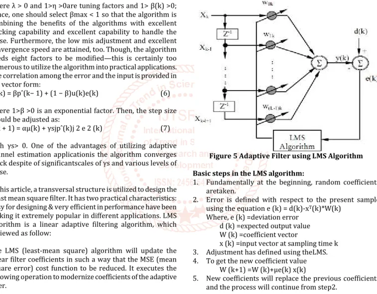
In this article, a transversal structure is utilized to design the Least mean square filter. It has two practical characteristics: Easy for designing & very efficient in performance have been making it extremely popular in different applications. LMS algorithm is a linear adaptive filtering algorithm, which reviewed as follow:

The LMS (least-mean square) algorithm will update the linear filter coefficients in such a way that the MSE (mean square error) cost function to be reduced. It executes the following operation to modernize coefficients of the adaptive filter.

Computes the error signal e (k) by utilizing the equation e (k) = d(k)-xT_{(k)*W(k) --- (1)}

Coefficient updating equation is

W (k+1) =W (k)+µe (k) x(k) --- (2) Where μ is the fixed step size of the adaptive filter u (k) is the input signal vector and (k) is the weight. The LMS ie least mean squares algorithm is one of the most famous algorithms in adaptive handling of the signal. Because of its robustness and minimalism was the focal point of many examinations, prompting its execution in

numerous applications. LMS algorithm is a linear adaptive filtering algorithm that fundamentally comprises of two filtering procedure, which includes calculation of a transverse filter delivered by a lot of tap inputs and creating an estimation error by contrasting this output with an ideal reaction. The subsequent advance is an adaptive procedure, which includes the programmed modifications of the tap loads of the channel as per the estimation error. The LMS algorithm is additionally utilized for refreshing channel coefficients. The benefits of the LMS algorithm are minimal calculations on the sophisticated nature, wonderful statistical reliability, straightforward structure, and simplicity of usage regarding equipment. LMS algorithm is experiencing problems regarding step size to defeat that EP ie evolutionary programming is utilized.

Figure 5 Adaptive Filter using LMS Algorithm Basic steps in the LMS algorithm:

1. Fundamentally at the beginning, random coefficients aretaken.

2. Error is defined with respect to the present sample using the equation e (k) = d(k)-xT_(k)*W(k)

Where, e (k) =deviation error d (k) =expected output value W (k) =coefficient vector

x (k) =input vector at sampling time k 3. Adjustment has defined using theLMS. 4. To get the new coefficient value

W (k+1) =W (k)+µe(k) x(k)

5. New coefficients will replace the previous coefficients and the process will continue from step2.

eqNew = comm.LinearEqualizer with the characteristics: Algorithm: 'LMS' WeightUpdatePeriod: 1 InitialWeightsSource: 'Auto' AdaptAfterTraining: true TrainingFlagInputPort: false InputSamplesPerSymbol: 2 InputDelay: 12 ReferenceTap: 6

Constellation: [0.7071 + 0.7071i 0.7071 + 0.7071i -0.7071 - -0.7071i -0.7071 - -0.7071i]

StepSize: 0.0100 NumTaps: 11

5. UPPER BOUND FOR THE STEP SIZE

Let's suppose that r is an upper bound on the number of different possible types of individuals, say a set Ω = {0, . . . , r − 1}. Such individuals can be strings, trees or whatever—our discussion is so general that the precise objects don’t matter. Even if the set of types can grow (such as trees) then practically speaking there will still be an upper bound r. The genetic system tries to solve an optimization problem in the following sense. Each individual in Ω is graded in terms of how well it solves the problem the genetic system is supposed to solve, expressed as a function f which maps Ω to some grading set G. For example, G can be the real interval [0, 1]. Let f(u) be the fitness oftype u. Then, the normalized fitness of individual u is ˆf(u) = f(u) P v∈Ω f(v) . To fix thoughts, we use fitness proportional selection where selection of individuals from a population is according to probability, related to the product of frequency of occurrence and fitness. That is, in a population P = (P(1), . . . , P(r)) of size n, where type u occurs with frequency P(u) ≥ 0 with P u∈Ω P(u) = n, we have probability p(u) to select individual u (with replacement) for the cross-over defined by p(u) = f(u)P(u) P v∈Ω f(v)P(v) . It is convenient to formulate the generation of one population from another one as a Markov chain. Formally A sequence of random variables (Xt) ∞ t=0 with outcomes in a finite state space T = {0, . . . , N−1} is a finite state time-homogeneous Markov chain if for every ordered pair i, j of states the quantity qi,j = Pr(Xt+1 = j|Xt = i) called the transition probability from state i to state j, is independent of t. If M is a Markov chain then its associated transition matrix Q is defined as Q := (qi,j ) N−1 i,j=0. The matrix Q is non-negative and stochastic, its row sums are all unity. Now let the Markov chain M have states consisting of nonnegative integer r-vectors of which the individual entries sum up to the population size exactly n and let P denote the set of states of M. The number of states N:= #P is given by [19] N = Ã n + r − 1 r − 1 ! .

Consider a process where the generation of a next population P 0 from the current population P consists of sampling two individuals u, v from P, removing these two individuals from P (P 00 := P −{u, v}), producing two new offspring w, z and inserting them in the population resulting in a population P 0 := P 00 S {w, z}. The transition probability qP,P0 of P → P 0 where P 0 results from sequentially executing the program “P(u) := P(u) − 1; P(v) := P(v) − 1;

P(w) := P(w) + 1; P(z) := P(z) + 1; P 0 := P,” replacing the pair of individuals u, v by w, z with {u, v} T {w, z} = ∅, is given by qP,P0 := 2p(u)p(v)b(u, v, w, z),

6. SIMULATED RESULTS

Statistical experimental method is a stochastic analysis method, which tests the dynamic characteristics of system and concludes the statistical results by mass data of computer simulations. The basic idea of problem solving is that a similar probability model should be built, then the statistical sampling should be carried out, the estimated values of sample should be considered as the approximate solution of original problem finally. The theoretical basis of statistical experimental method is law of large numbers, and the main method is the sampling analysis of random variables [7-11]. Simulation analysis should be carried out to visually display the LMS algorithm. Input signal is the synthesis signal, which is synthesized by a sine signal and a white noise signal. X(n) = √ 2s(n) + sqrt(10− SNR 10 )j(n) (3) Where s(n) is the sine signal, j(n) is the Gaussian white noise signal (average value is zero, power is one). The Gaussian white noise signal can form an interference cancellation system. It is noteworthy that there is not any time-delay in the LMS algorithm, because the correlation function of Gaussian white noise signal is the impulse function, the correlativity will disappear when the time-delay exists in the expected signal and input signal. Simulation conditions are shown in Table 1. Simulation results are shown in Figure 6. The results indicate that the convergence performances of LMS algorithm are prefect, the input signal canconverge to the expected signal (sine signal ornoise signal). Besides, the convergence speed and performances of LMS algorithm have great relationship with the length of filter and step factor. The simulation results show that the error rate of system with an adaptive equalizer has significant improvement gains over that of system without an adaptive equalizer. The smaller the error rate, the larger the SNR. The relationship between error rate and multi-path loss show thatthe error rate is largest when the loss factor is 0.5, which means the transmission paths of two signals are in the most interferential conditions. The simulation results accord well with the theoretical analysis.

In Figure 6, comparative convergence natures of optimized equalizers EPLMS along with equalizers prompted by ABC and ACO algorithms have been implemented for the various input signal. From the figure,it is clear that theproposed EPLMS performs more iterations with reduced time. Additionally, it was observed that amongst optimized Aes, EPLMS equalizer is the fastest one.

Table 1: BER Values Input Signal SNR ->

BER 4 8 16 20

EPLMS Equalizer 0.450e-01 0.769e-02 0.899e-04 0.698e-05 ACO-Equalizer 8.785e-02 1.264e-02 3.000 e-05 6.789 e-06 ABC-Equalizer 9.448e-02 9.930e-03 1.890 e-05 2.783 e-056

0 2 4 6 8 10 12 0 10 20 30 40 50 60 70 80 90 100 SNR B E R ABC-Equalizer ACO-Equalizer EPLMS

Figure 7 Comparison of BER act of EPLMS optimized equalizer with ABC and ACO equalizers for various input Signals

Figure 7shows that the EPLMS AEs disclose well BER acts in comparison to the AEs with ABC and ACO specificallythe greater SNR area. The comprehensive outcomes have been outlined in Table1.

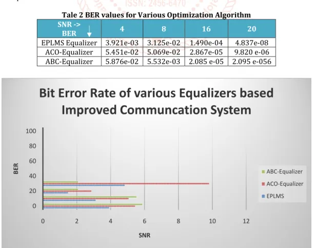
Tale 2 BER values for Various Optimization Algorithm SNR ->

BER 4 8 16 20

EPLMS Equalizer 3.921e-03 3.125e-02 1.490e-04 4.837e-08 ACO-Equalizer 5.451e-02 5.069e-02 2.867e-05 9.820 e-06 ABC-Equalizer 5.876e-02 5.532e-03 2.085 e-05 2.095 e-056

0 2 4 6 8 10 12 0 20 40 60 80 100 SNR B E R

Bit Error Rate of various Equalizers based

Improved Communcation System

ABC-Equalizer ACO-Equalizer EPLMS

From Figure 8 and Table 2, it has been noticed that the EPLMS equalizer effectively retains its superiority over ACO and ABC triggered AEs in improved communication systems. For illustration, EPLMS equalizers express the BER values of 43.125e-02 for an SNR value of 8 dB; whereas, ACOand ABC generated AEs to offer BER values of 5.069 e-02 and 5.532 e-03 for similar SNR value. More obviously, it was distinguished that the order of improvement in BER behavior of the EPLMS based EP improved communication system is viewed to be 101 over ABC and ACO based improved communication systems; however, the proportion increase in BER value utilizing EPLMS based improved communication system is observed to be 23.15%. In connection with this20 dB SNR level was deemed. Analogous improvements have also been observed for lower SNR segments. Henceforth, it can be clearly agreed that EPLMS optimized AEs surpass the AEs synchronized by ACO and ABC methods. Though, EPLMS optimized AE provides the optimal result amongst all the combinations.

7. CONCLUSION

The efficiency of the contemporary communication system can be decreased by the non-ideal feature of the channel, which is referred to as the ISI (inter-symbol interference).The equalization method is an effective technique to defeat the ISI and enhance the features of the system. Adaptive linear filter and several types of training algorithms are utilized to imitate various equalizer models. Here a digital communication model has been simulated which contains LMS algorithm along with evolutionary programming which is implemented in MATLAB in which the Equalizer performs a most important position in this model. In our design, since we are using evolutionary programming it will decide what would be the value of step size for a particular application so that (Mean Square Error) MSE is minimized and convergence is optimal. And also, faster convergence is obtained. Consequently, we can enhance the effectiveness of an interaction system. Several adaptive algorithms were intended to attain low BER, quick tracking, and high-speed convergence rate in previous two years. This article reviewed LMS algorithms along with evolutionary programming & offered a performance comparison by means of wide-ranging simulation with ABC and ACO. A comprehensive review offers that the EPLMS triggered Adaptive Equalizers (AEs) to offer quicker convergence act in comparison with ABC and ACO structures. Additionally, optimized equalizers are propelled by EPLMS techniques also demonstrate theirpre-eminence in accordance with the conditions of BER performance over the ABC and ACO algorithms. Moreover, it has also been observed that EPLMS is better for ABC and ACO optimized AEs. With the layout of the obtaining filters, we can reduce the impact of Inter symbol Interference.

REFERENCES

[1] Gupta, Anubha, and ShivDutt Joshi. "Variable step-size LMS algorithm for fractal signals." IEEE Transactions

on Signal Processing 56.4 (2008): 1411-1420.

[2] Li, Ting-Ting, Min Shi, and Qing-Ming Yi. "An

improved variable step-size LMS algorithm." 2011 7th

International Conference on Wireless Communications,

Networking and Mobile Computing. IEEE, 2011.

[3] Zhao, Haiquan, et al. "A new normalized LMAT

algorithm and its performance analysis." Signal

processing 105 (2014): 399-409.

[4] Wang, Yixia, Xue Sun, and Le Liu. "A variable step size LMS adaptive filtering algorithm based on L2 norm." 2016 IEEE International Conference on Signal

Processing, Communications and Computing (ICSPCC).

IEEE, 2016.

[5] Jamel, Thamer M. "Performance enhancement of

adaptive acoustic echo canceller using a new time varying step size LMS algorithm (NVSSLMS)." International Journal of Advancements in Computing

Technology (IJACT) 3.1 (2013).

[6] Aref, Amin, and MojtabaLotfizad. "Variable step size

modified clipped LMS algorithm." 2015 2nd

International Conference on Knowledge-Based

Engineering and Innovation (KBEI). IEEE, 2015.

[7] Sun, En-Chang, et al. "Adaptive variable-step size LMS filtering algorithm and its analysis." Journal of System

Simulation 19.14 (2007): 3172-3174.

[8] Dixit, Shubhra, and Deepak Nagaria. "LMS Adaptive

Filters for Noise Cancellation: A Review." International Journal of Electrical & Computer

Engineering (2088-8708) 7.5 (2017).

[9] Zhang, Zhong-hua, and Duan-jin Zhang. "New variable

step size LMS adaptive filtering algorithm and its performance analysis." systems Engineering and

Electronics 31.9 (2009): 2238-2241.

[10] Xu, Kai, Hong Ji, and Guang-xin YUE. "A modified LMS

algorithm for variable step size adaptive filters."

Journal of Circuits and Systems 4 (2004).

[11] Zhao, Haiquan, and Yi Yu. "Novel adaptive VSS-NLMS

algorithm for system identification." 2013 Fourth International Conference on Intelligent Control and