Rongfeng Zhang
Abstract
Diffractions in seismic data indicate discontinuities of the subsurface, although they are often obscured by and difficult to separate from the more prominent reflection events. A seismic section containing only diffractions could therefore be of great signifi-cance for the interpretation of seismic data. Here, some techniques such as dip filtering and Radon transform are adapted and used to extract diffractions from prestack seis-mic data. Final diffraction stack sections will be shown and possible applications are discussed. Both synthetic model examples and a real and complicated data set example are illustrated. We also show that not only can the identification of the discontinuities in structure be enhanced, but, also, the resolution may be dramatically improved in contrast to the traditional definition of resolution in seismology.
1
Introduction
Small and complex structure imaging is now gaining interest and stead in both academic and industry applications. Tremendous development and progress of relevant techniques such as prestack depth migration (PSDM), super-computer modeling and lithology inversion has, as a consequence, resulted. In spite of this progress, it appears that seismic diffractions, although essential for a good imaging, are rarely separately taken into account, especially in oil and gas exploration. In fact, diffractions are sometimes even considered as noise as, for example, in ground penetrating radar (GPR). As we will see later on, except for PSDM, conventional data processing largely favours reflections over diffractions. In other words, reflections, already strong, are enhanced even more than diffractions during the processing. This reflection-centered methodology tends to distort the weak diffractions during processing. Only when reflections are removed therefore, or at least attenuated, can the potentially unique value of diffractions be revealed following diffraction specific processing.
Actually, as early as 1952, Krey [5] considered applications involving diffractions. Harris et al. [1] in 1996, Landa et al. [6] in 1998 and Khaidukov et al. [3] in 2003 used diffractions
0 0.5 1.0 1.5 time(s) 100 200 300 400 (a) 0 0.5 1.0 1.5 time(s) 100 200 300 400 (b)
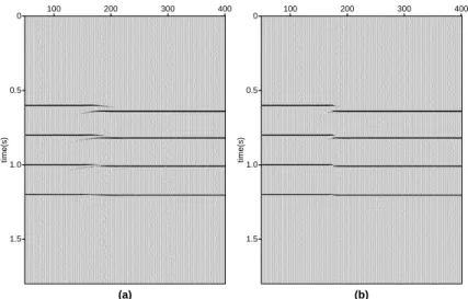
Figure 1: Vertical resolution illustration. (a) and (b) are stacked and migrated sections respectively. The ratios of the vertical throw to the wavelength are 1,0.5,0.25 and 0.125 from top to bottom reflections.
to detect inhomogeneities or scattering objects, and even imaging (Khaidukov et al. [4] in 2003 used a focusing-defocusing approach). What would result if diffractions were treated separately in routine seismic data processing? We will show that clear, high-resolution images of discontinuities such as faults and edges of pinchouts can be achieved.
By high-resolution, we actually mean super-resolution, when compared to the traditional definition of resolution. Typically, the vertical resolution of seismic exploration is defined as a quarter of the dominant wavelength
λ= υ
f (1)
whereυ is the velocity and f is the dominant frequency, which varies with both the medium and the source properties. Practically, we assume half wave length as a reasonable value for resolution. Figure 1 shows, from top to bottom, four reflections with different vertical throw (1, 1
2, 14 and 18 of wavelength). Figure 1 (a) is the stacked section and Figure 1 (b) is the migrated section. It can be seen that only faults with a vertical throw larger than 1 4 wavelength can be reliably resolved.
Lateral resolution is defined as Fresnel zone [2]
r= υ
2 s
t0
f (2)
the vertical travel time. This is slightly more complicated than the vertical resolution. Since
t0 is included, lateral resolution is also related to the distance from the source.
As the following sections will show, diffractions can provide higher resolution than that of the above convention. This is a striking but not surprising fact: if the size of an object is close to the wavelength, the dominant energy will be the diffracted rather than reflected. Reflections can, in fact, totally disappear. This phenomenon is well known in physics but is not fully utilized in exploration seismology.
2
Separation of diffractions and reflections
Diffractions and reflections have different characteristics, such as amplitude and travel time, which facilitates their separation. Complete separation is only possible in very rare cases, but, from a practical point of view, it is not necessary to completely eliminate the reflections. Our aim is to reveal the potential of diffractions — some part of reflections may remain as long as the diffractions are not masked.
Generally speaking, NMO, an adaptive dip-filter, migration, and de-migration operators will be used to suppress reflections. The procedure for suppressing reflections free of steep dipping reflection events is:
1. Sort the data into the common middle point (CMP) domain; perform velocity analysis, picking the velocities that correspond to reflections including multiples. Note that the velocity does not have to be monotonically increasing with time as required in normal velocity analysis.
2. Apply NMO corrections based on the velocities picked above. 3. Resort the data into the common shot point domain.
4. Apply an adaptive dip-filter to each shot gather, with dip angle chosen close to zero. 5. Resort the data to the CMP domain and apply inverse NMO correction using the same
velocity estimated at step 1.
6. Process the data as one requires, such as re-estimating primary velocity (based on diffractions) and NMO corrections and then stack, or even prestack depth migration.
Unlike conventional applications, the dip-filtering here used is basically to filter out the horizontal strong events since the reflections after NMO correction become the strong flat events. We found that the data have to be tapered on both sides in order to decreasing strong artifacts due to the filtering. This procedure was incorporated into the dip-filtering, obtaining much better results. We use the term adaptive dip-filtering. Figure 6 shows the effect of the tapering.
In case the data contain steep dipping reflection events, the procedure is modified to: 1. Sort the data into the CMP domain; perform velocity analysis, picking the velocities
corresponding to reflections including multiples. As before the velocity does not have to be monotonically increasing with time.
2. Apply NMO corrections based on the velocities picked above. 3. Resort the data into the common shot point domain.
4. Apply a linear Radon transform, filtering out the reflections in Radon domain then transform back.
5. Resort the data to the CMP domain and apply inverse NMO corrections using the same velocities estimated in step 1.
6. Process the data as required, such as re-estimating primary velocity (based on diffrac-tions) and NMO corrections and then stack, or even prestack depth migration.
The former procedure can very efficiently separate diffractions and reflections without af-fecting diffractions but is not suitable for arbitrary sections; the latter procedure can work on any sections but some reflection energy will be left in the section after filtering.
It is known that the reflection events of both the flat and the dipping reflectors in CMP domain are hyperbolae with apex located at zero offset. After NMO correction, the responses of flat reflectors will be flattened if the correct RMS velocity v0 is used, but events of the dipping reflectors are not flattened using the same velocity. However, if the velocity is adjusted by the dip angleα, that is
v = v0
cos(α) (3)
then those events corresponding to dipping reflections can also be flattened. This is also true for diffraction events and consequently this approach is not suitable to differentiate them.
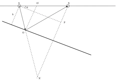
h O P α X / X S O/
Figure 2: Geometry of a single dipping reflector. αis the dip angle. S and X stands for the source and
the receiver respectively. X0 is the mirror point of X for the dipping reflector. O is the reflecting point on
the dipping reflector. his the distance between S and the dipping reflector. P is the perpendicular projection
point of S onXX0. O0 is the intersecting point of the normal line of the dipping plane with the surface.
However, we found that dipping reflection responses in the common shot gather domain will become dipping linear events if they are NMO corrected using RMS velocity without angle adjustment. First, we derive the travel time equation of a dipping reflector in common shot gather domain. For a flat reflector
t= 1
v
√
x2+ 4h2 (4)
wherev is the RMS velocity,h is the distance between the surface and the reflector,xis the offset (the distance between the source and the receiver) and t is the two-way travel time. For a dipping reflector, the travel time equation can be deduced from Figure 2 as
t= 1 v q x2+ 4hx·sin(α) + 4h2 (5) or t= 1 v q (x+ 2h·sin(α))2 + 4h2cos2(α) (6)
where h is the vertical distance between the source and the dipping reflector and α is the dip angle. It is a hyperbola with a shifted apex in−2h·sin(α). Appendix A gives the detail of the derivation. From the appendix, the travel time equation after NMO correction (using
a two term approximation) of a flat reflector and dipping reflector are tN M O = 2h v − 1 64 1 h3vx 4 −O(x6) (7) and tN M O = h(1 + cos2(a)) cos (a)v + sin (a)x cos (a)v + (1−cos (a))x2
4hcos (a)v +O(x
4) (8)
respectively. It is clear that ifxis not too large, the travel time for the flat reflector becomes a horizontal line as expected
tN M O ≈
2h
v (9)
but when α6= 0 , i.e. the dipping reflector, the linear term in equation can’t be ignored but higher order terms can be, so we have
tN M O ≈
h(1 + cos2(a))
cos (a)v +
sin (a)x
cos (a)v (10)
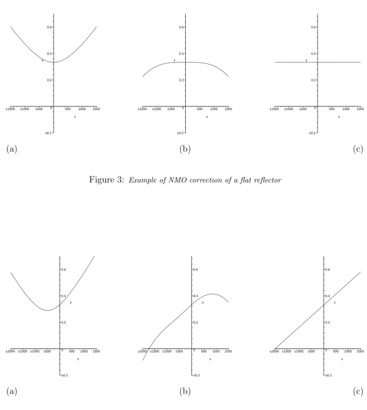
which is a dipping straight line. It is easy to see that ifα= 0 the result for dipping reflector is identical to that for a flat reflector. Figure 3 and Figure 4 show the numerical results. Figure 3 (a) shows the travel time curve for a flat reflector. It is a hyperbola with apex located at the zero offset. After NMO correction using a two-term approximation, the result is shown in Figure 3(b), which is a flat straight line in near and middle offsets, and Figure 3(c) shows the ideal corrected line. Similarly Figure 4 (a) shows the travel time curve of a dipping reflector (α = 300) which is a shifted hyperbola. Figure 4(b) shows the NMO corrected result which is a dipping straight line in the center portion. Figure 4(c) shows the ideal dipping straight line.
It must be pointed out that if higher terms are used in the NMO correction, the ideal results as shown in Figure 3 (c) and Figure 4 (c) are expected.
A linear Radon transform is now used to filter out those reflections after NMO correction. To achieve this, we developed a special strategy which will be illustrated with examples in section 3.5.
3
Synthetic data examples
The examples will show the reflection-suppressed or diffraction-only image and demonstrate the processing procedure and illustrate why conventional processing affects diffractions.
–0.2 0 0.2 0.4 0.6 y –1500 –1000 –500 500 1000 1500 x –0.2 0 0.2 0.4 0.6 y –1500 –1000 –500 500 1000 1500 x –0.2 0 0.2 0.4 0.6 y –1500 –1000 –500 500 1000 1500 x (a) (b) (c)
Figure 3: Example of NMO correction of a flat reflector
–0.2 0 0.2 0.4 0.6 y –2000 –1500 –1000 –500 500 1000 1500 x –0.2 0 0.2 0.4 0.6 y –2000 –1500 –1000 –500 500 1000 1500 x –0.2 0 0.2 0.4 0.6 y –2000 –1500 –1000 –500 500 1000 1500 x (a) (b) (c)
3.1
Example 1
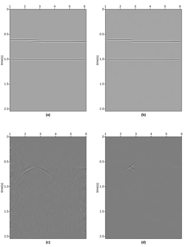
Figure 5 shows a simple example. The data do not contain multiples but do contain a small amount of noise. Figure 5(a) is the stack section of a simple three-layer structure with first reflection containing a small fault. The vertical throw of the fault is one wavelength. Figure 5(b) is the poststack time migrated section of Figure 5(a). Obviously, in Figure 5(a) the diffractions are obscured by strong reflections. When the reflections are removed, a clear diffraction section, Figure 5(c), results. After migration, Figure 5(d), the accurate location of the fault is depicted. The phase property of the migrated dots provide even more information about the property of the fault. Specifically, when comparing the two dots in Figure 5 (d), the top one is different from the bottom one in terms of positive to negative transition or phase feature.
Figure 6 shows an individual gather. Figure 6(a) is the original gather; Figure 6(b) is the reflection-suppressed gather using the adaptive dip-filter; 6(c) is the reflection-suppressed gather using normal dip-filtering. Clearly, the adaptive dip-filtering result does not exhibit the artifacts such as the strong four dots in Figure 6(c), caused by the strong boundary effects of the prominent reflections.
In this simple example, we are able to completely remove reflections, although as stated previously, this is not a stringent requirement.
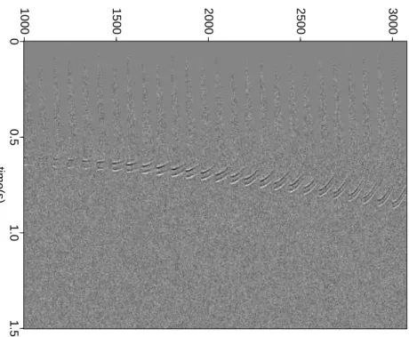
It should be pointed out that the stacking velocities used for NMO correction are picked from the reflection events as usual. The processing of Figure 5 and Figure 6 are all based on this velocity. However, this is definitely not correct for diffraction stacking. Figure 7 shows some NMO corrected and reflection-suppressed CMP gathers. Note that at some locations the diffractions are flattened, but at many locations they are not. Thus, when stacking them together, loss of diffraction energy is inevitable.
It is not surprising that there is a noticeable change when diffraction stacking velocity is used to stack diffractions. Figure 8 shows the comparison. Figure 8(a) shows the diffraction stack section stacked using reflection stacking velocity; 8(b) shows the diffraction stack section stacked using diffraction stacking velocity; 8(c) shows the poststack migrated section of 8(a); 8(d) shows the poststack migrated section of 8(b). Both stack section and migrated section have a remarkable change. In Figures 8(a) and 8(b), the flank, especially the right flank, of the diffractions have gained clarity. The artifacts just left to the apex in Figure 8(a) due to the wrong velocity used has disappeared in Figure 8(b). Compared to Figure 8(c), the focusing of the diffractions in Figure 8(d) is much better and, consequently, the
0 0.5 1.0 1.5 2.0 time(s) 1 2 3 4 5 6 (a) 0 0.5 1.0 1.5 2.0 time(s) 1 2 3 4 5 6 (b) 0 0.5 1.0 1.5 2.0 time(s) 1 2 3 4 5 6 (c) 0 0.5 1.0 1.5 2.0 time(s) 1 2 3 4 5 6 (d)
Figure 5: A three-layer structure example. (a) stack section; (b) poststack time migrated section; (c) the stack section of extracted diffractions; (d) the poststack time migrated section of Figure (c).
(a) (b) (c)
Figure 6: One gather in example 1 shows improvement due to the adaptive dip-filter. (a) is the original gather; (b) is the reflection-suppressed gather using normal dip-filtering; (c) is the reflection-suppressed gather using the adaptive dip-filtering.
0 0.5 1.0 1.5 time(s) 1000 1500 2000 2500 3000
resolution has been improved.
In this example, the maximum CMP fold is just 16. It can be expected that if the fold number increases, the differences will be more accentuated.
3.2
Example 2
This is a slightly complicated model. Figure 9 (a) shows the model that contains a multi-layer structure with a sink in the middle. Figure 9(b) shows three shot gathers of the synthetic data of this model. Besides the prominent four reflection events, there are many other events which are the diffractions. These diffractions are information-rich.
Figure 10 shows the stack section and migrated section respectively. Figure 10(a) shows the stack section. Figure 10(b) shows the poststack time migrated section of Figure 10(a). Obviously, in Figure 10(a) the diffractions are obscured by strong reflections. When the reflections are removed, a clear diffraction section, Figure 10 (c), stands out. After migration, Figure 10(d), the accurate location of the sink is depicted. Note that the phase properties of the focused points reflect the characteristics of the different points in the sink structure. In this example, the reflection stacking velocity is used for stacking both reflections and diffractions. As Figure 8 demonstrates, the result can be improved if diffraction stacking velocities are used.
3.3
Example 3
Diffractions can reveal features that reflections cannot under normal resolution limitations. Figure 11 shows a special example. Figure 11(a) and Figure 11(c) are the stack section and migrated section respectively through conventional processing which takes into account both reflections and diffractions. The model consists of two reflecting horizons with the first horizon containing a tiny fault whose vertical throw is just 1 meter, or 1
40 wavelength. It should not be surprising that this fault is totally absent in Figures 11 (a) and Figure 11(c) as it is far below the resolution limit. However Figures 11(b) and Figure 11(d), the diffraction stack section and the migrated diffraction section, respectively, clearly show the response of this fault.
To further challenge the resolution potential of diffractions, we slightly modified the the model so that the vertical throw is -1 meter which means the footwall and the hangingwall have been exchanged. The results are shown in Figure 12 (b) and Figure 13 (b). They are
0 0.5 1.0 1.5 2.0 time(s) 1 2 3 4 5 6 (a) 0 0.5 1.0 1.5 2.0 time(s) 1 2 3 4 5 6 (b) 0 0.5 1.0 1.5 2.0 time(s) 1 2 3 4 5 6 (c) 0 0.5 1.0 1.5 2.0 time(s) 1 2 3 4 5 6 (d)
Figure 8: Comparison between stacking using reflection velocity and using diffraction velocity. (a) is the diffraction stack section stacked using reflection stacking velocity; (b) is the diffraction stack section stacked using diffraction stacking velocity; (c) is the poststack migrated section of (a); (d) is the poststack migrated section of (b).
0 500 1000 1500 Depth (m) 500 1000 1500 (a) . 0 0.5 1.0 1.5 time(s) (b)
0 0.5 1.0 1.5 2.0 time(s) 1 2 3 4 5 6 (a) 0 0.5 1.0 1.5 2.0 time(s) 1 2 3 4 5 6 (b) 0 0.5 1.0 1.5 2.0 time(s) 1 2 3 4 5 6 (c) 0 0.5 1.0 1.5 2.0 time(s) 1 2 3 4 5 6 (d)
Figure 10: Stack section and migrated section of model (a) stack section; (b) poststack time migrated section; (c) the stack section of extracted diffraction; (d) the poststack time migrated section of Figure (c)
0 0.5 1.0 1.5 2.0 time(s) 0.5 1.0 1.5 2.0 (a) 0 0.5 1.0 1.5 2.0 time(s) 0.5 1.0 1.5 2.0 (b) 0 0.5 1.0 1.5 2.0 time(s) 0.5 1.0 1.5 2.0 (c) 0 0.5 1.0 1.5 2.0 time(s) 0.5 1.0 1.5 2.0 (d)
Figure 11: A tiny fault example. (a) the stack section which contains both reflections and diffractions; (b) the diffraction stack section only; (c) is the migrated section of (a), and (d) is the migrated section of (b).
0 0.2 0.4 0.6 0.8 1.0 1.2 1.4 time(s) 0.5 1.0 1.5 2.0 (a) 0 0.2 0.4 0.6 0.8 1.0 1.2 1.4 time(s) 0.5 1.0 1.5 2.0 (b) 0 0.2 0.4 0.6 0.8 1.0 1.2 1.4 time(s) 0.5 1.0 1.5 2.0 (c)
Figure 12: Diffraction stack sections of different tiny faults. (a) diffraction stack section of the fault with 1 meter vertical throw, (b) diffraction stack section of the fault with -1 meter vertical throw and (c) diffraction stack section of fault with zero vertical throw but has 1 meter horizontal discontinuity. All figures show events above 1.5 second.
the stack section and migrated section respectively. In addition, Figure 12 (d) and Figure 13 (d) show the response of the similar model but the vertical throw is zero and the first reflection has a 1 meter discontinuity at the same horizontal location as the other two models. Surprisingly, these three models that differ only slightly from each other, can be resolved and differentiated by means of the phase properties of the processed sections. Since there is no any difference in the conventional processed sections, they are not shown here.
3.4
Example 4
Figure 14 shows a classic geology structure, pinchout, example. The accurate determination of the edge of a pinchout is significant in data processing and interpretation. Figure 14(a) is the stack section of the pinchout. Figure 14(b) is the poststack time migrated section of Figure 14(a). Obviously, in Figure 14(a) the diffractions are obscured by prominent reflections. The exact edge of the pinchout is difficult to determine. When the reflections are removed, a clear diffraction section, Figure 14(c), results. After migration, Figure 14 (d), the accurate location of the pinching-out point can be determined.
0 0.2 0.4 0.6 0.8 time(s) 0.5 1.0 1.5 2.0 (a) 0 0.2 0.4 0.6 0.8 time(s) 0.5 1.0 1.5 2.0 (b) 0 0.2 0.4 0.6 0.8 time(s) 0.5 1.0 1.5 2.0 (c)
Figure 13: Diffraction migrated sections of different tiny faults. (a), (b) and (c) are corresponding migrated section of Figure 12 (a), Figure 12 (b) and Figure 12 (c). All figures show events above 1.0 second.
3.5
Dipping event examples
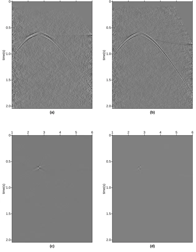
As introduced and proved in previous sections that, although a dipping event in a shot gather is hyperbolic in shape, after NMO correction, it becomes linear. As seen in Figure 15, Figure 15 (a) is the original shot gather that contains a flat reflection event, a dipping reflection event and a diffraction event. After NMO correction, as shown in Figure 15(b), the flat reflection event becomes a flat linear event and the dipping reflection event becomes a dipping linear event. Naturally, linear Radon transform was implemented to attenuate these events. Figure 15(c) shows the same data as in Figure 15(b) but in the linear Radon domain. As expected, those linear events which correspond to reflection events collapse to two dots. Simply muting out these dots, the reflections will be removed. However, we have to be careful, because those dots are not spikes in real data or even in this simple synthetic data that contains a small amount of noise. The noise, the finite aperture and banded spectra etc. are all factors which contribute to the specific patterns exhibited by the dots, as seen in Figure 15(d), which shows the same data as in Figure 15(c) but with different plot parameters to enhance the weak energy. This type of behaviour is also seen in multiple attenuation using the Radon transform.
To overcome this problem, a special strategy has been developed, which is outlined below:
0 0.5 1.0 1.5 2.0 time(s) 1 2 3 4 5 6 (a) 0 0.5 1.0 1.5 2.0 time(s) 1 2 3 4 5 6 (b) 0 0.5 1.0 1.5 2.0 time(s) 1 2 3 4 5 6 (c) 0 0.5 1.0 1.5 2.0 time(s) 1 2 3 4 5 6 (d)
Figure 14: Pinchout example. (a) stack section; (b) poststack time migrated section of (a); (c) the stack section of extracted diffraction; (d) the poststack time migrated section of Figure (c)
0 0.5 1.0 1.5 2.0 time(s) 0 500 1000 offset (a) 0 0.5 1.0 1.5 2.0 time(s) 0 500 1000 offset (b) 0 0.5 1.0 1.5 2.0 time(s) 0 200 400 600 800 1000 offset (c) 0 0.5 1.0 1.5 2.0 time(s) 0 200 400 600 800 1000 offset (d)
Figure 15: A single shot gather containing a dipping event. (a) The original shot gather; (b) After NMO correction; (c) After linear Radon transform; (d) The same as (c) except using different plot parameters to boost weak energy.
• Apply linear Radon transform to each shot gather;
• Manually or automatically pick the reflections in Radon domain; We actually developed an approach to automatically pick the points.
• We then have two ways to go: (1). We have the approach:
– From the picked points, we know the (τ, p ) values and we can generate those linear events in the original (x, t) domain based on these values and the specified wavelets.
– Apply the same linear Radon transform to the synthetic gather generated in the previous step. Thus, a similar patter in Radon domain of this synthetic gather to the pattern of the original data can be expected. For example, both events in (x, t) domain have the same finite aperture.
– Subtract the synthetic gather in the Radon domain from the the original data in the Radon domain entirely or just around the picked points. The latter is preferred because the synthetics may not be accurate.
(2). If the reflection events have subtle variations or the wavelets can not be accurately estimated, the above procedure may not work well. In this case, another approach is:
– From the picked points, knowing their (τ,p) values, we pick out the corresponding linear events in the original gather in the (x, t) domain based on these values and combine them together as a “picked gather”. Note that this is not a synthetic gather. Ideally, it has all the characteristics of the original reflections including the waveforms and apertures etc.
– Apply the same linear Radon transform to the picked gather generated in the previous step. Thus, a similar pattern in the Radon domain of this gather to the pattern of the original data can be expected.
– Subtract the picked gather in the Radon domain from the the original data in the Radon domain entirely or just around the picked points. The latter is preferred because of errors involved in any of the above steps.
Figure 16 illustrate this procedure. Figure 16 (a) is the same as Figure 15 (d) except that the two reflection dots are simply muted. Figure 16(b) and Figure 16(c) show the result of the complicated muting introduced above. They differ only in the subtraction. The subtraction of Figure 16(b) is carried on on entire section while, in Figure 16(c) it is only done around the picked points. Note that the slant events in the plots are the diffractions. Figures 16(d), 16(e) and 16(f) are the corresponding gathers in the (x, t) domain to Figure 16(a), 16(b) and 16(c), respectively. Clearly, the new subtraction approach works much better than simple muting.
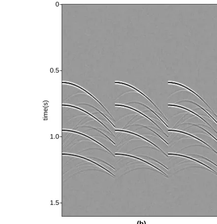
Figure 17 shows a model with one flat and two dipping events and the result of processing. The dipping events have opposite dip angles. Figure 17(b) shows the stack section. Figure 17 (c) shows the stack section processed by the linear Radon transform introduced above. After filtering, the two diffraction events stand out clearly.
4
Real data example
A real data example is given here in order to show what a real data diffraction section looks like. Figure 18 shows the conventional stack and post-stack time migrated sections of a 2D line from the Mississippi area, Gulf of Mexico. As expected, the salt top generates the strongest diffractions (at approximately 3 seconds). This is because the salt body has a large velocity contrast with the sediment environment and has many small fractures. The diffractions are so strong that even the multiples contain diffractions (at approximately 4 and 4.6 seconds) which becomes a big challenge for multiple attenuation. Figure 19 shows the stack and post-stack time migrated diffraction sections. From these figures, we get a clear diffraction image. A huge amount of diffractions are seen at the top of the salt. The diffraction multiples are clear. In addition, a few diffractions close to the sea bottom (at 2.2 seconds) are especially interesting. They clearly show the locations of the shallow faults that are obscured by the strong sea bottom reflections. Note the above post-stack time migrated sections are generated by F-K migration using constant velocity.
5
PSDM result
In case accurate velocities are known, PSDM can always give better results. Here, PSDM can be applied to the extracted diffractions to obtain a superior image.
0 0.5 1.0 time(s) 1.5 2.0 0 200 400 600 800 1000 offset (a) 0 0.5 1.0 time(s) 1.5 2.0 0 200 400 600 800 1000 offset (b) 0 0.5 1.0 time(s) 1.5 2.0 0 200 400 600 800 1000 offset (c) 0 0.5 1.0 time(s) 1.5 2.0 0 500 1000 offset (d) 0 0.5 1.0 time(s) 1.5 2.0 0 500 1000 offset (e) 0 0.5 1.0 time(s) 1.5 2.0 0 500 1000 offset (f)
Figure 16: Illustration of a special approach for attenuating reflections. (a), (b) and (c) are in linear
Radon domain and their corresponding figures in the (x, t) domain are shown in (e), (f) and (g) respectively.
0 0.5 1.0 1.5 2.0 time(s) 500 1000 1500 2000 2500 CMP (a) 0 0.5 1.0 1.5 2.0 time(s) 500 1000 1500 2000 2500 CMP (b) 0 0.5 1.0 1.5 2.0 time(s) 500 1000 1500 2000 2500 CMP (c)
Figure 17: A synthetic model with two dipping events and its diffraction extraction result. (a) the model containing a flat reflector but with a small fault, and two dipping reflectors; (b) the stack section of the response of (a) and (c) shows the diffraction stack section.
Figure 20 shows a moderate complex synthetic model experiment. Figure 20(a) shows Kirch-hoff PSDM result of the original data, and Figure 20(b) shows the KirchKirch-hoff PSDM result of the diffraction data. This model tries to model a small salt body embedded in a sediment environment. The sediment layer structure comes with several faults. Especially there are two small faults underneath the salt body. One (right side), with 4m vertical throw, can hardly be identified in Figure 20(a), and another one (left side), with 2m vertical throw, is totally absent in Figure 20(a). They are too small to be within the conventional resolution. In Figure 20(b), not only do the big faults and the embedded salt body stand out, but also the two tiny faults beneath the salt body can be clearly identified. Note that there are several missing steep parts of the salt body. This is because standard Kirchhoff PSDM that we used here does not use the full wavefield. In other words, it does not take full advantage of the diffraction data.
Since diffractions are weaker than reflections, noise will clearly have a larger impact on diffractions than reflections. Figure 21 shows another experiment to test the influence of noise. 20% by amplitude of noise was added to the data. Figure 21 (a) shows Kirchhoff PSDM result of the original data, and Figure 21(b) shows the Kirchhoff PSDM result of the diffraction data. Although a large amount of noise has been added, Figure 21(b) still shows meaningful result.
0 500 1000 1500 Depth(m) 500 1000 1500 2000 2500 3000 Distance(m) (a) 0 500 1000 1500 Depth(m) 500 1000 1500 2000 2500 3000 Distance(m) (b)
Figure 20: Moderately complex synthetic model with tiny faults. (a) Kirchhoff PSDM result of the original data; (b) the Kirchhoff PSDM result of the diffraction data.
0 500 1000 1500 Depth(m) 500 1000 1500 2000 2500 3000 Distance(m) (a) 0 500 1000 1500 Depth(m) 500 1000 1500 2000 2500 3000 Distance(m) (b)
Figure 21: Synthetic experiment with 20% added noise. (a) Kirchhoff PSDM result of the original data; (b) Kirchhoff PSDM result of the diffraction data.
6
Discussion and conclusions
In this report we describe a procedure by means of which we have attempted to remove all reflected energy so that the diffractions present in the section can stand out. In practice, and fortunately so, it is only required that the reflection energy is attenuated to the same level as that of the diffractions.
We have to bear in mind that the premise of diffraction imaging is the existence of discon-tinuities that can generate noticeable diffractions. Therefore, a smooth subsurface structure will not benefit from this technique. However imaging of discontinuities such as faults and unconformity points, especially their accurate location, is a very important task in explo-ration.
Diffractions are considerably more susceptible to noise than are reflections since the energy of diffractions is weaker than that of reflections. As a result, diffraction imaging is not suitable for strongly noise contaminated data. More CMP folds are always helpful. Note that the CMP folds used in our synthetic examples are very low. Real data normally have larger CMP folds. In addition, it is recommended that a split-spread geometry be adopted in acquisition for better recordings of diffractions.
Diffraction imaging, if used in reflection seismology, can generate not just different but higher resolution results. It is a process suitable for discontinuity identification and imaging. It can be incorporated into conventional data processing flow, but requires special attention in data interpretation. We believe that diffraction imaging would facilitate the work of the interpreter, especially in the solution and clarification of problems associated with complex structure.
A special strategy based on the linear Radon transform has also been developed to attenuate reflections. Obviously the underling idea of this strategy can be applied to other similar problems, such as multiple attenuation.
Acknowledgments
References
[1] J. M. Harris and G. Y. Wang. Diffraction tomography for inhomogeneities in layered background medium. In Geophysics, volume 61, pages 570–583. Soc. of Expl. Geophys., 1996.
[2] F. J. Hilterman. Interpretative lessons from three-dimensional modeling. In Geophysics, volume 47, pages 784–808. Soc. of Expl. Geophys., 1982.
[3] V. Khaidukov and E. Landa. Scattering Objects Detection Using Diffraction Imaging, page E08. Eur. Assn. Geosci. Eng., 2003.
[4] V. Khaidukov and T. Moser. Diffraction imaging by a focusing-defocusing approach, pages 1094–1097. Soc. of Expl. Geophys., 2003.
[5] T. Krey. The significance of diffraction in the investigation of faults. In Geophysics, volume 17, pages 843–858. Soc. of Expl. Geophys., 1952.
[6] E. Landa and S. Keydar. Seismic monitoring of diffraction images for detection of local heterogeneities. In Geophysics, volume 63, pages 1093–1100. Soc. of Expl. Geophys., 1998.
A
Travel time equation in common shot gather of a
dip-ping reflector and its NMO corrected expressions
Figure 2 shows the geometry of a dipping reflector with dip angleα. S andX stands for the source and the receiver respectively. X0 is the mirror point of X for the dipping reflector. O
is the reflecting point on the dipping reflector. h is the distance between S and the dipping reflector. P is the perpendicular projection of S on XX0. O0 is the intersection point of the
normal line of the dipping plane with the surface. From the figure, the travel time from S toX can be written as t= SO+OX v = SO+OX0 v , since 6 XOX0+6 OXX0+6 XX0O = 1800 6 SOO0 =6 O0OX 6 O0OX =6 OXX0 then 6 SOX0 = 1800 then t= SX 0 v = 1 v √ SP2+P X02 where SP =cos(α) and P X0 =XX0−x·sin(α) = 2h+xsin(α), so SX02 =x2+ 4h2+ 4hxsin(α)
and the travel time becomes
t= 1
v q
x2+ 4hsin(α) + 4h2.
Its NMO correction using the two-term approximation is
tN M O = 1 v q x2+ 4hsin(α) + 4h2− x2 4vh = 4h q x2+ 4hsin(α) + 4h2−x2 4vh
Expanding it to tN M O = 2h v (cos(α)− 1 2sin 2(α)) + sin(α) v (x+ 2hsin(α)) +( 1 4hvcos(α) − 1 4vh)(x+ 2hsin(α)) 2+O((x+ 2hsin(α))4) = h(1 + cos 2(a)) cos (a)v + sin (a)x cos (a)v + (1−cos (a))x2
4hcos (a)v +O(x+ 2hsin(α))
4).
Obviously the linear term cossin((αα))v will disappear if the dip angle α approaches zero and it reduces to the travel time equation for a flat reflector.