Residual diagnostics for interpreting CUB models

RESIDUAL DIAGNOSTICS FOR INTERPRETING CUB MODELS1

F. Di Iorio, M. Iannario

1. INTRODUCTION

In ordinary linear regression, graphical diagnostics can be very useful for de-tecting anomalous features in a fitted model (Atkinson, 1985; Belsey et al., 1980; Cook and Weisberg, 1994; Daniel and Wood, 1971; Fox, 1991, 1997; Weisberg, 1980). This validation step is pursued by residual analysis and it is worth consider-ing for several purposes: to check the structure of the model, verifyconsider-ing the nature and persistence of the postulated dependence, to detect outliers and/or influen-tial data, to assess the validity of classical linear hypotheses (homoscedastic and uncorrelated errors), to test distributional assumptions (Gaussianity, for instance) or shape behaviours (skewness, heavy tails), and so on.

However, when the response variable is not continuous (and specifically of categorical nature), it is difficult to interpret the usual definition of residuals and the related graphical devices. In fact, the results are invariably discrete and stan-dard techniques are not very effective. The problem has been mainly raised in the framework of Generalized Linear Models (GLM), as proposed by McCullagh (1980) and McCullagh and Nelder (1989). In this context, the definition of general-ized residuals have been derived by first-order conditions of the maximum likeli-hood equations (Lanweher, Pregibon and Shoemaker, 1984).

The specification and extensions of residual diagnostics to categorical and or-dinal data have been successfully pursued with ordered polytomous (probit and logit) analysis, as in Pregibon (1981). In this regard, Agresti (2010) synthesizes several approaches, and we mention the standardized residuals given by the ratio of the difference between the observed and the fitted values and the standard error of difference under the hypothesis that the model is correct. In addition, it can be informative to quote the residuals obtained by cumulative totals and referred to as Pearson-type residuals. In relation to this frame, Liu et al. (2009) proposed graphi-cal diagnostics based on cumulative sums of residuals to check the misspecifica-tion of the propormisspecifica-tional odd models. Moreover, Pruscha (1994) suggested partial

residuals whereas Bender and Benner (2002) introduced a smoothed partial resid-ual plot.

Other issues related to the analysis of residuals from a fitted model, have been obtained by using univariate and bivariate marginal distributions: Bartholomew and Tzamourani (1999) and Jöreskog and Moustaki (2001), among others. Finally, Lindsay and Roeder (1992) introduced residual diagnostics for mixture models.

In this paper, we analyze residual diagnostics with reference to ordinal data modelled by means of CUB models (Piccolo, 2003; D’Elia and Piccolo, 2005; Iannario, 2012; Iannario and Piccolo, 2012). More specifically, we define esti-mated residuals, their transformations and related graphical methods and then ex-tend the concept of binned residuals (Gelman and Hill, 2007) to CUB models. Re-sidual plots, based on first-order conditions of maximum likelihood equations, have been previously discussed by Di Iorio and Piccolo (2009).

The paper is organized as follows: the formulation and some basic features of CUB models are considered in section 2. Section 3 proposes a definition of re-siduals for such mixture models whereas section 4 introduces binned residual plots. Section 5 checks the usefulness of such device by means of empirical data set. Section 6 contains some final remarks.

2. BACKGROUND AND NOTATION

We analyze ordinal responses expressed on the support {1,2,...,m} where m>3 for identifiability purposes (Iannario, 2010). To be specific, we consider ratings data r =(r1, r2,..., rn)’ as the collection of scores assigned by a sample of n raters to a prefixed item.

Formally, CUB models2 _{are specified by considering the observed sample r of}

responsesas n realizations of a discrete random variable R whose probability dis-tribution is a mixture of Uniform and shifted Binomial random variables, both defined on the support {1,2,...,m}.

For improving fitting and interpretation, a logistic link among the parameters and some selected subjects’ covariates is conveniently assumed. The parameters of a CUB model (denoted by ư and Ʈ, respectively) are inversely related to uncer-tainty and feeling features of respondents, respectively. Instead, the observations of subjects’ covariates are collected for the two components in the matrices Y and W, respectively. Further details have been discussed by Iannario and Piccolo (2012).

Then, information for explaining the rating ri of the i-th subject, for i=1,2,...,n, is:

1 2 1 2

( |1,ri yi , yi , ,! yip|1,w wi , i , ,! wiq) .

It is related to parameters by the systematic links:

1 1

= ( ) = ; = ( ) = ; = 1, 2, , ,

1 i 1 i

i i _e yE i i _e wJ i n

S S E [ [ J

! (1)

where yi and wi are the covariates of the i-th subject for explaining Si and [i, re-spectively, and Ƣ= ( , , ,E E0 1! Ep) ; = ( , , , ) ,c ƣ J J0 1 ! Jq c are the vectors of the pa-rameter vectors (supposed fixed across individuals) for yi and wi, respectively.

As a consequence, for a given m>3, the probability distribution of a CUB model with p covariates for explaining uncertainty and q covariates for explaining feeling, hereafter denoted as CUB(p,q) model, turns out to be:

1 1

1 ( )

1 1 1

( = | , , , ) = .

1

1 (1 )

w_i r_i

i i i y_i w_{i m}

i

m e

Pr R r y w

r m m

e e J E J E J

ª§ · º

«¨ ¸ »

«_¬© ¹ »_¼ (2)

Given the sample information In=(r | Y | W ), if we let ƨ=(Ƣ´, ƣ´ )´ the set of all

p+q+2 parameters to be estimated, then the log-likelihood function is defined by:

=1

)

log ( | ) =_n n log[ ( = | , , ]._{i i i} i

L T I

¦

Notice that, for obtaining maximum likelihood (ML) estimates, an effective maximization approach to (3) is required and this is based on EM algorithm (Piccolo, 2006).

In order to assess the closeness between the observed responses and the fitted values, goodness-of-fit statistics have been introduced in the literature. Some of them are based on deviance and divergence measures (Cameron and Windmeijer, 1997; Hastie, 1987; McCullagh and Nelder, 1989) and these criteria are particu-larly useful in presence of covariates for comparing nested models.

When covariates are absent, the absolute differences between the probability

ˆ ˆ

( = | ) r( )

Pr R r T p T , evaluated by the estimated CUB model, and the corre-sponding observed relative frequency fr, r=1,2,...,m are often used as inverse measures of goodness of fit. Such quantities may be considered as starting points for building dissimilarity indexes (Leti, 1979; Simonoff, 2003) or direct normal-ized fitting measures as:

2

1

ˆ

1

1 | ( )|.

2 m

r r

r

F

_¦

An alternative normalized measure:

1 2 2 1 ˆ 1 1 1 ( ) m r r r f L

m p T

ª _{§ ·} º

« _{¨ ¸} »

« _{© ¹} »

has been proposed by Iannario (2009). This index has been derived by a first-order property of ML estimates.

As already mentioned, inferential issues for this class of models have been pur-sued by ML methods, and the related asymptotic inference may be applied by us-ing variance and covariance matrix of estimators (with ML estimates plugged in). Alternatively, nonparametric inference has been introduced in order to check the adequacy of an estimated model or to compare nested CUB models obtained for small sample size (Arboretti et al. 2011; Bonnini et al. 2011).

3. GENERALIZED RESIDUALS IN CUB MODELS

In a previous work, Di Iorio and Piccolo (2009) discussed generalized residuals for CUB models for uncertainty and feeling covariates. They defined, for i=1,2,...,n, the quantities:

( ) _ˆ

ˆ

1

(1 ( )) 1

( ) i i i e m p S S E T § · _{¨ ¸}

© ¹ (4)

( ) ˆ _ˆ

ˆ

1

1 ( ( 1) ( ))

( )

i i i

i

e m r m

m p [ S [ J T § · ¨ ¸

© ¹ (5)

which may be considered as ML generalized residuals with respect to ưi and Ʈi,

respectively. They are obtained from first-order conditions of ML equations and may be useful to investigate where and how significant covariates affect single probabilities. Notice that these quantities assume a number of different values depending on the number of modalities of covariates.

Hereafter, we introduce a different definition of residuals for CUB models which is more similar to the standard regression framework. For simplicity, we consider the common case where only the feeling parameter Ʈ is explained by co-variates W. Thus, the discussion is limited to CUB(0,q) models.

We define residuals as: ei=Ri - E(Ri|W=wi; ƨ) and their estimates as:

i

ˆe ri E R W( |i wi; ),T i 1, 2,..., .n

Since the expectation of a CUB model is: ( ) = ( 1) 1 ( 1)

2 2

m E R S m §_¨ [·_¸

© ¹ ,

given that covariates affect only the feeling parameter Ʈ, from (1), the previous residuals may be expressed as:

i ˆ ˆ

( 1)

1

ˆe ( 1) ( ) , 1, 2,..., .

2 2

i i

m

r ªS m § [ J · º i n

_{« ¨ ¸ »}

© ¹

¬ ¼ (6)

of ˆe is yet conditioned to _i Sˆ but the explicit reference to p_i( )Tˆ in denominators

– as it happens in definitions (4) and (5) – disappeared. Thus, small probabilities are not so influential on the residual computations.

Notice that:

( )_i ( _i ( |_{i i}; )) ( )_i ( |_{i i}; ) 0;

E e E R E R W w T E R E R W w T

2 2

1 1

( ) ( ) ( 1) ( 1) tanh ;

4 3 2

(1 )

i

i

A

i

i i A

A

e m

V e Var R m m

e

S

S S

ª § ª _{§ ·} º·º

« »

¨_¨ « ¨ ¸ »¸_¸

© ¹

« © «¬ »¼¹»

¬ ¼

where Ai=-wiƣ. Thus, the residuals (6) are heteroscedastic.

4. BINNED RESIDUAL PLOTS

In order to avoid the discrete pattern in the residual plot, which is the conse-quence of the ordinal nature of responses, we introduce a binned residual plot for CUB models according to similar proposals for dichotomous data.

Suppose that X is the variable we use to define J bins for plotting averaged re-siduals belonging to the selected j-th bin, for j=1,2,...,J. Such variable may be a subjects’ covariate (or a combination of them) but also a probability computed by the estimated CUB models.

To be consistent, we define the i-th residual belonging to the j-th bin as:

[ ], 1, 2,..., ; 1, 2,..., .

i j j

e i n j J

Typically, there is some arbitrariness in choosing the number of bins: we want enough points so that the averaged residuals are not so noisy, but it helps to have many bins to see more local patterns in the residuals. In this regard, it is a com-mon practice to specify ni as a constant value ( n, say) but some bins may pos-ses different size; so, our notation is taking this generalization into account.

Another approach would be to apply a nonparametric smoothing procedure such as lowess (locally weighted scatterplot smoothing: Cleveland, 1979). It com-bines the simplicity of linear least squares regression with the flexibity of nonlin-ear regression by fitting simple models to local subsets of data to build a function that describes the deterministic variation in the data.

The graphical device we are discussing about is a representation of the average of njobserved realizations of ei j[ ] for each group (bin) selected according to the

ordered values of a prefixed variable X. Then, the binned residuals are given by:

[ ] 1

1 nj _{, 1, 2,..., .}

j i j

i j

e e j J

This random variable is characterized by:

2 [ ] 1

1

( ) 0; ( ) , 1, 2,..., ,

j

n

j j i j

i j

E e Var e j J

n

¦

where we denoted by 2 [ ]

i j

V the variance of a CUB random variable (Piccolo, 2003) conditioned by the observed value of the X variable for the i–th subject.

Thus, to obtain a binned residual plot we order data with respect to the X variable into categories (bins), and then we plot the average residual versus the average value of the variable for each bin. Specifically, each point of the binned residual plot is specified by an abscissa computed on some average of X and an ordinate com-puted on the realizations of ej.

The asymptotic standard-error bounds, within which one would expect about 95% of the binned residuals to fall if the model is assumed to be true, are:

2 [ ]

1.96 i j , 1, 2,..., .

j

j J

n

V r

5. SOME EMPIRICAL EVIDENCE

To verify the effectiveness of the proposal we implement the analysis of binned residual plots for CUB models on a real data set. Specifically, we analyze a subset of ISFOL-2006 data by considering 20184 subjects which expressed their perception of subjective survival probabilities to 75 years; such data have been transformed in a qualitative assessment about the personal perception to survive by means of a Likert scale with m=7. For illustrative purposes, we refer to models fitted to such data and already discussed in Di Iorio and Piccolo (2009), Iannario and Piccolo (2010).

In the estimated CUB models, only the Gender, the deviations and the squared deviations of logarithm of Age turned out to be relevant covariates for explaining the feeling parameter, and the main results are reported in Table 1. As we can see, the inclusion of covariates for feeling parameter Ʈ does not sensibly modify the estimation of Sˆ, whereas significantly improves the goodness of fit measures (as shown by the increase of estimated log-likelihood functions and the correspond-ing reductions of BIC).

TABLE 1

CUB models for subjective survival probabilities to age 75

Models Parameter Estimates Log-likel. BIC

CUB(0,0) Sˆ 0.867(0.005) [ˆ 0.163(0.001) -30383 60782.3

CUB(0,1) Sˆ 0.865(0.005) Jˆ0 1.642(0.011) -30365 60754.5

Log(Age) Jˆ1 0.135(0.023)

CUB(0,2) Sˆ 0.867(0.005) Jˆ0 1.522(0.015) -30310 60652.7

Log(Age) Jˆ1 0.125(0.024)

[Log(Age)]2

2

ˆ 0.682(0.065)

J

CUB(0,3) Sˆ 0.868(0.005) Jˆ0 1.598(0.020) -30291 60622.8

Log(Age) Jˆ1 0.108(0.024)

[Log(Age)]2 Jˆ₂ 0.616(0.066)

Gender Jˆ3 0.121(0.020)

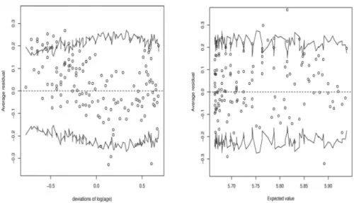
In the left panel of Figure 1, we observe a quadratic (parabolic) structure, which disappears in the right panel after the introduction of deviations of squared logarithm of age. Specifically, we observe that about 10% of the binned residuals corresponding to small values of the deviance of log(Age) exceeds the upper level of confidence bound.

Figure 1 – Binned residuals for [parameter with covariates Age (left panel) and Age2 _{(right panel).}

In addition, in the right panel of Figure 2, we report another kind of residual plot in which we observe the relationship between average residuals and expected values of the rating scores. In the left panel, a moderate amount of residuals falls outside of the dotted 95% confidence bands for the residual plot, whereas in the right panel just few binned residuals are located out of the confidence bands. Thus, such representations summarize and support the quality of the estimation.

Finally, if we compare the graphical devices for the same data set reported by Di Iorio and Piccolo (2009), and based on (4) and (5) definitions of residuals, it seems evident that Figures 1-2 depict in a sharper manner the information ob-tained by the model diagnostics step.

Figure 2 – Binned residuals for [parameter vs average of Age and expected values.

6. CONCLUDING REMARKS

In this work, we have discussed the role of residuals obtained by fitting CUB models to ordinal data as diagnostic tools for improving the interpretation and checking the effect of covariates. The binned residual plot seems a convenient trick to avoid the discreteness nature of such data which hides useful relation-ships and prevent from the detection of influential behaviors.

In this regard, further studies are necessary in order to explore related issues, as the effect of different size of bins since the arbitrariness in choosing the number of bins (see Gelman and Hill, 2007, pag. 97) may affect some conclusions. Inves-tigations of several data sets are important but also simulation studies should be performed in order to test the real effectiveness of such new diagnostic tools.

Department of Theory and Methods of Human FRANCESCA DI IORIO

and Social Sciences, Statistical Sciences Section MARIA IANNARIO

REFERENCES

A. AGRESTI, (2010), Analysis of ordinal categorical data, 2nd edition, J. Wiley & Sons, New Jer-sey.

R. ARBORETTI, S. BONNINI, M. IANNARIO, F. SOLMI, (2011), Permutation test approach for the analysis of rating data, Proceeding of SIS Meeting, Bologna.

A. C. ATKINSON, (1985), Plots, transformations, and regressions: an introduction to graphical methods of diagnostic regression analysis, Clarendon Press, Oxford.

D. J. BARTHOLOMEW, P. TZAMOURANI, (1999), The goodness of fit of latent trait models in attitude measurement, “Sociological Methods and Research”, 27:525-546.

D. A. BELSEY, E. KUH, R. E. WELSCH, (1980), Regression diagnostics: identifiying influential data and sources of collinearity, J. Wiley & Sons, New York.

R. BENDER, A. BENNER, (2000), Calculating ordinal regression models in SAS and S-Plus, “Biomet-rical Journal”, 42:677-699.

S. BONNINI, D. PICCOLO, L. SALMASO, F. SOLMI, (2011), Permutation inference for a class of mixture models, “Communications in Statistics. Theory and Methods”, forthcoming.

A. C. CAMERON, F. A. G. WINDMEIJER, (1997), An R-squared measure of goodness of fit for some com-mon nonlinear regression models, “Journal of Econometrics”, 77:329-342.

W. S. CLEVELAND, (1979), Robust locally weighted regression and smoothing scatterplots, “Journal of the American Statistical Association”, 74:829-836.

R. D. COOK, S. WEISBERG, (1994), An introduction to regression graphics, J. Wiley & Sons, New York.

C. DANIEL, F. S. WOOD, (1971), Fitting equation to data, J. Wiley & Sons, New York.

A. D’ELIA, D. PICCOLO, (2005), A mixture model for preference data analysis, “Computational Sta-tistics & Data Analysis”, 49:917-934.

F. DI IORIO, D. PICCOLO, (2009), Generalized residuals in CUB models: definition and applications, “Quaderni di Statistica”, 11:73-88.

J. FOX, (1991), Regression diagnostics: an introduction, Sage, Newbury Park, CA.

J. FOX, (1997), Applied regression analysis, linear models, and related methods, Sage, Thousand Oaks.

A. GELMAN, J. HILL, (2007), Data Analysis using Regression and Multilevel/Hierarchical Models, Cambridge University Press, New York.

T. HASTIE, (1987), A closer look at deviance, “The American Statistician”, 41:16-20.

M. IANNARIO, (2009), Fitting measures for ordinal data models, “Quaderni di Statistica”, 11:39-72.

M. IANNARIO, (2010), On the identifiability of a mixture model for ordinal data, “METRON”, LXVIII: 87-94.

M. IANNARIO, (2012), Modelling shelter choices in a class of mixture models for ordinal responses, “Sta-tistical Methods and Applications”, 21, 1-22.

M. IANNARIO, D. PICCOLO, (2010), Statistical modelling of subjective survival probabilities, “GE-NUS”, LXVI:17-42.

M. IANNARIO, D. PICCOLO, (2012), CUB models: Statistical methods and empirical evidence, in: R.S. KENETT, S. SALINI (eds.) “Modern Analysis of Customer Surveys: with application using R”, J. Wiley & Sons, New York, 231-258.

K. JÖRESKOG, I. MOUSTAKI, (2001), Factor analysis of ordinal variables: A comparison of three ap-proaches, “Multivariate Behavioral Research”, 36:347-387.

J. M. LANWEHER, D. PREGIBON, A. C. SHOEMAKER, (1984), Graphical methods for assessing logistic re-gression models, “Journal of the American Statistical Association”, 79:61-83.

B. G. LINDSAY, K. ROEDER, (1992), Residual diagnostics for mixture models, “Journal of the Ameri-can Statistical Association”, 87:785-792.

I. LIU, B. MUKHERJEE, T. SUESSE, D. SPARROW, S. K. PARK, (2009), Graphical diagnostics to check model misspecification for the proportional odds regression model. “Statistics in Medicine”, 28:412-429. P. MCCULLAGH, (1980), Regression models for ordinal data (with discussion), “Journal of the Royal

Statistical Society, Series B”, 42:109-142.

P. MCCULLAGH, J. A. NELDER, (1998), Generalized linear models, 2nd edition, Chapman & Hall, London.

D. PICCOLO, (2003), On the moments of a mixture of uniform and shifted binomial random variables, “Quaderni di Statistica”, 5:85-104.

D. PICCOLO, (2006), Observed information matrix for MUB models, “Quaderni di Statistica”, 8:33-78.

D. PREGIBON, (1981), Logistic regression diagnostics, “The Annals of Statistics”, 9:705-724. H. PURSCHA, (1994), Partial residuals in cumulative regression models for ordinal data, “Statistical

Papers”, 35:273-284.

S. WEISBERG, (1980), Applied linear regression, J. Wiley & Sons, New York. J. S. SIMONOFF, (2003), Analyzing categorical data, Springer, New York.

SUMMARY

Residual diagnostics for interpreting CUB models