ISSN: 1311-1728 (printed version); ISSN: 1314-8060 (on-line version)
doi:http://dx.doi.org/10.12732/ijam.v31i3.11
GLOBAL STABILITY ANALYSIS FOR LASSA FEVER TRANSMISSION DYNAMICS WITH
OPTIMAL CONTROL APPLICATION O.S. Obabiyi1, Akindele A. Onifade2§
1,2Department of Mathematics University of Ibadan
Ibadan, NIGERIA
Abstract: A mathematical model for transmission dynamics of Lassa fever with optimal control application is presented. The existence of region where the model is epidemiologically feasible is established with respect to the use of pesticide control measure. We use personal protection control measure and basic reproduction number in linear and nonlinear Lyapunov functions together with the Lasalle’s invariant principle to show that disease free and endemic equilibria are globally asymptotically stable. The existence and uniqueness of an optimality system are discussed. A characterization of the optimal control via adjoint variables is established. The possible impact of using combinations of the three controls either one at a time or two at a time or three at a time on the spread of the disease is also examined.
AMS Subject Classification: 92B05, 93A30
Key Words: mathematical model, reservoir host, global stability, reproduc-tion number, optimal control
1. Introduction
Lassa fever is an acute viral illness that occur in West Africa. The virus, a member of the virus family arenaviridae is a zonotic or animal borne. In
Received: May 3, 2018 c 2018 Academic Publications
other words, the well-known Lassa fever is mostly caused by the Lassa virus. The symptoms include flu-like illness characterized by fever, general weakness, cough, sore throat, headache, and gastrointestinal manifestations, [12]. Ac-cording to the World Health Organization, 300 000 to 500 000 cases of Lassa fever and 5000 deaths occur yearly across West Africa, [13]. The major and most common lesion of Lassa fever in humans occurs in the liver, [1, 2, 4, 5]. There are a number of ways in which the virus can be transmitted or spread to humans. The Mastomys rodents shed the virus in urine and droppings. There-fore, the virus can be transmitted through direct contact with these materials, touching objects or eating food contaminated with these materials, or through cuts or sores. Because Mastomys rodents often live in and around homes and scavenge on human food remains or poorly stored food, transmission of this sort is common. Contact with the virus also may occur when a person inhales tiny particles in the air contaminated with rodent excretions. This is called aerosol or airborne transmission.
Finally, because Mastomys rodents are sometimes consumed as a food source, infection may occur via direct contact when they are caught and pre-pared for food. Lassa fever may also spread through person-to-person contact. This type of transmission occurs when a person comes into contact with virus in the blood, tissue, secretions, or excretions of an individual infected with the Lassa virus. The virus cannot be spread through casual contact (including skin-to-skin contact without exchange of body fluids). Person-to-person trans-mission is common in both village and health care settings, where, along with the above-mentioned modes of transmission, the virus also may be spread in contaminated medical equipment, such as reused needles (this is called nosoco-mial transmission).
To put this research into proper perspective, we briefly give an account of some existing literatures on mathematical study of Lassa fever. D. Okuonghae and R. Okuonghae [8] discussed a mathematical model for the transmission of Lassa fever. Steady states of their model were examined for epidemic and endemic situations. The results of their model show that in the interim control of the rodents carrying the virus and some isolation policy for the infected individuals are the best strategies against the spread of the disease.
Bawa et al. [7] developed a mathematical model for Lassa fever transmission dynamics in two interacting population. They obtained the basic reproduction number and stability of the disease free equilibrium was established. The results of their work suggest that every effort must be put in place by all concerned to prevent the virus infection by reducing reproduction number.
trans-mission dynamics. They obtained the basic reproduction number which can be used to control the transmission dynamics of the disease and conditions for local stability of the disease free equilibrium was established.
Onuorah, Akinwande et al. [10] developed a mathematical model for Lassa fever as a six dimensional system of nonlinear ordinary differential equation with rigorous analyzes. The results of their analysis and numerical simulation show the effects of the control parameters on the various compartments of the model and conclude that if the basic reproduction number is low the disease will still continue to spread.
2. A Model for Optimal Control of Lassa Fever
We introduce the control functionsu1(t),u2(t), andu3(t) for prevention, treat-ment and use of pesticide respectively on a time interval [0, T]. Known practices of prevention are use of rodent-proof container, use of infection control measure such as complete equipment sterilization, improving home hygiene and strict barrier nursing such as masks, gloves, gowns and goggles to prevent human to human contact. Ribavirin the antiviral drug is effective in the treatment of Lassa fever but only if administered early in the course of illness, [6].
Consequently, 1−u1(t) describes the failure of prevention effort for t≥0;
α1 and α2 are the treatment rates of exposed and infected class respectively. We assumed that 0≤u2(t)≤1 to eliminate the case where the entire infected and exposed classes are treated effectively. Use of pesticide in and around homes can help reduce rodent population denoted by 1−u3(t). The model subdivides the total human population size at time t and discrete age ai de-noted by Nh(t, ai) with i = 0,1,2, ..., L and aL is the maximum age of hu-mans in the population, into susceptible huhu-mans Sh(t, ai), exposed humans
Eh(t, ai), infected humans Ih(t, ai) and recovered humansRh(t, ai). Hence we have Nh(t, ai) = Sh(t, ai) +Eh(t, ai) +Ih(t, ai) +Rh(t, ai). A loss of individ-uals is as a result of infection and natural death µh(ai)Sh(t, ai). The exposed human gain individuals through infection and loses individual when they be-come infectedǫh(ai)Eh(t, ai) and to natural deathµh(ai)Eh(t, ai). The infected human Ih(t, ai) gain individuals when exposed individuals becomes infected and loses individual when they die µh(ai)Ih(t, ai) and disease induced death
susceptible human Sh(t, ai) are susceptible,θ(ej) ∝ KvCv and θ(ej) is generated from urine and faeces of infectious rodents, whereCv is the amount of virus in air and Kv is the saturation of virus in air. Similarly,κ(ai) is generated from blood of infectious individuals,κ(ai) ∝ AvSv, whereAv is the amount of virus in needle and Sv is the saturation of virus in needle.
In a similar manner, we subdivides the total rodent population size at time t and discrete age ej denoted by Nr(t, ej) with j = 0,1,2, ..., T and
eT is the maximum age of rodents in the population, into susceptible rodents
Sr(t, ej), exposed rodentsEr(t, ej) and infected rodentsIr(t, ej). Hence we have
Nr(t, ej) =Sr(t, ej) +Er(t, ej) +Ir(t, ej). Susceptible rodent classSr(t, ej) gain more individual into rodent population by input rate Λr(ej), while it loses ro-dents through infection, natural death µr(ej)Sr(t, ej), hunting δr(ej)Sr(t, ej). Transmission of Lassa virus to susceptible rodents occurs when they share un-protected storage of garbage, food stuff and water with infected rodents or from inhalation of aerosols from urine. When a susceptible rodent interacts with infectious rodent, the virus enters the rodent with probability β(ej) and therefore the susceptible go to the exposed class Er(t, ej). The exposed rodent then becomes infectious and enters the class Ir(t, ei) after a given time. It is assumed that the recruitment rate of rodent is greater than rodent’s number of death at initial time (Λr(ej)≥µr(ej)Nr(0, ej)). In this study, it is assumed that individuals who recovered from Lassa fever will never go back to suscep-tible class again (they remain recovered for life). Thus, the transition dynamic is given by:
dSh(t, ai)
dt = Λh(ai)
− L
X
i=0 T
X
j=0
ρ(ai)σ1(ej)Ir(t, ej) +η(ai)σ2(ai)Ih(t, ai) +θ(ej) +κ(ai)
Nh(t, ai)
×Sh(t, ai)(1−u1(t))−µh(ai)Sh(t, ai), (1)
dEh(t, ai)
dt =
L
X
i=0 T
X
j=0
ρ(ai)σ1(ej)Ir(t, ej) +η(ai)σ2(ai)Ih(t, ai) +θ(ej) +κ(ai)
Nh
dIh(t, ai)
dt =
L
X
i=0
ǫh(ai)Eh(t, ai)−(ψ(ai)α2(ai)u2(t) +µh(ai) +δh(ai))Ih(t, ai), (3)
dRh(t, ai)
dt =
L
X
i=0
[γ(ai)α1(ai)u2Eh(t, ai) +ψ(ai)α2(ai)u2(t)Ih(t, ai)]−µh(ai)Rh(t, ai), (4)
dSr(t, ej)
dt = Λr(ej)
− T
X
j=0
β(ej)σ1(ej)Ir(t, ej) +θ(ej)
Nr(t, ej)
(1−u3(t))Sr(t, ej)
−(µr(ej) +δr(ej) + (1−u3(t)))Sr(t, ej), (5)
dEr(t, ej)
dt =
T
X
j=0
β(ej)σ1(ej)Ir(t, ej) +θ(ej)
Nr(t, ej)
(1−u3(t))Sr(t, ej)
−(ǫr(ej) +µr(ej) +δr(ej) + (1−u3(t)))Er(t, ej), (6)
dIr(t, ej)
dt =
T
X
j=0
ǫr(ej)Er(t, ej)−(µr(ej) +δr(ej) + (1−u3(t)))Ir(t, ej). (7)
2.1. Existence of Solutions
First, we obtain boundedness of the state system given an optimal control set U.
Theorem 2.1. Givenu1(t), u2(t) and u3(t)∈ U, the state equations
(2.1)-(2.7) has a bounded positive solution on feasible invariant region Rdefined by
Nh(0, ai)≤Nh(t, ai)≤ L
X
i=0
Λh(t, ai)
µh(ai) ,
Nr(0, ej)≤Nr(t, ej)≤ T
X
j=0
Λr(ej)
µr(ej) +δr(ej) + (1−u3)
with initial conditions Sh(0, ai)≥0, Eh(0, ai)≥0, Ih(0, ai)≥0,Rh(0, ai)≥0,
Sr(0, ej)≥0, Er(0, ej)≥0, Ir(0, ej)≥0.
Proof.If the total human population size is given byNh(t, ai) =Sh(t, ai) +
Eh(t, ai)+Ih(t, ai)+Rh(t, ai) and the total size of rodent population isNr(t, ej) =
Sr(t, ej) +Er(t, ej) +Ir(t, ej), then the system (2.5)-(2.7) gives
dNr(t, ej)
dt ≤Λr(ej)−
T
X
j=0
(µr(ej) +δr(ej) + (1−u3(t)))Nr(t, ej), (8)
and therefore the equation (2.8) leads to
Nr(t, ej)e(µr(ej)+δr(ej)+(1−u3(t))t ≤
T
X
j=0
Nr(0, ej) + Λr(ej)
µr(ej) +δr(ej) + (1−u3)
e(µr(ej)+δr(ej)+(1−u3(t))t
− Λr(ej)
µr(ej) +δr(ej) + (1−u3(t))
,
so that
Nr(t, ej)≤ T
X
j=0
Nr(0, ej)e−(µr(ej)+δr(ej)+(1−u3(t))t
+ Λr(ej)
µr(ej) +δr(ej) + (1−u3(t))
− Λr(ej)
µr(ej) +δ(ej) + (1−u3(t))
e−(µr(ej)+δr(ej)+(1−u3(t))t.
This implies
Nr(t, ej)≤ T
X
j=0
Λr(ej)
µr(ej) +δr(ej) + (1−u3(t))
×(1−e−(µr(ej)+δr(ej)+(1−u3(t))t
)
Taking the limit as t→ ∞ gives
Nr(t, ej)≤ T
X
j=0
Λr(ej)
µr(ej) +δr(ej) + (1−u3(t))
.
Similarly, from equations (2.1)-(2.4) we obtain
dNh(t, ai)
dt ≤Λh(ai)−
L
X
i=0
µh(ai)Nh(t, ai), (9)
and the inequality (2.9) gives
Nh(t, ai)eµh(ai)t≤ L
X
i=0
Nh(0, ai) + Λh(ai)
µh(ai)
eµh(ai)t−Λh(ai)
µh(ai), so that
Nh(t, ai)≤ L
X
i=0
Nh(0, ai)e−µh(ai)t+ Λh(ai)
µh(ai)
−Λh(ai)
µh(ai)e
−µh(ai)t.
This implies
Nh(t, ai)≤ L
X
i=0
Λh(ai)
µh(ai)
(1−e−µh(ai)t) +Nh(0, ai)e−µh(ai)t.
Taking the limit as t→ ∞ gives Nh(t, ai) ≤ L
X
i=0
Λh(t, ai)
µh(ai) . Thus, we have the following feasible region
R={Sh(t, ai), Eh(t, ai), Ih(t, ai), Rh(t, ai), Sr(t, ej), Er(t, ej), Ir(t, ej)∈ R7 :
Nr(t, ej)≤ T
X
j=0
Λr(ej)
µr(ej) +δr(ej) + (1−u3(t))
, Nh(t, ai)≤ L
X
i=0
Λh(ai)
µh(ai)
}.
2.2. Disease-Free Equilibrium Stable and Reproduction Number The system (2.1)-(2.7) has a disease-free equilibrium given by
π0 =
Λh(ai)
µh(ai)
,0,0,0, Λr(ej)
µr(ej) +δr(ej) + (1−u3)
,0,0
. (10)
Using the next generation matrix operator approach, we obtain the basic re-production number as,
R0(a) = L
X
i=0
η(ai)σ2(ai)ǫh(ai)
(γ(ai)α1(ai) +ǫh(ai) +µh(ai))(ψ(ai)α2(ai) +µh(ai) +δh(ai))
2.3. Global Stability of Disease Free Equilibrium
In this sub-section, we show that disease free equilibrium is globally asymptot-ically stable (GAS) with respect to only the range of prevention control.
Theorem 2.2. The disease-free equilibrium π0 of the model (2.1)-(2.7), is globally asymptotically stable inRif R0(a)≤1for all aand0≤u1(t)≤1 for
all t.
Proof. To determine global stability of the disease-free state, consider the following linear Lyapunov function
L= ǫh(ai)Eh(t, ai)
(µr(ej) +δr(ej))(ǫh(ai) +γ(ai)α1(ai)u2+µh(ai))qt
+ Ih(t, ai)
(µr(ej) +δr(ej))(ψ(ai)α2(ai)u2+µh(ai) +δh(ai)) + Er(t, ej)
Λr(ej)(β(ej)σ1(ej) +θ(ej))
+ Ir(t, ej)(ǫr(ej) +µr(ej) +δr(ej)) (β(ej)σ1(ej) +θ(ej))Λr(ej)ǫr(ej)
, (12)
whereqt= (ψ(ai)α2(ai)u2+µh(ai) +δh(ai)). The Lyapunov derivative (2.12) is given by
˙ L=
L
X
i=0 T
X
j=0
ǫh(ai)(ρ(ai)σ1(ej)Ir(t, ej) +θ(ej) +κ(ai))(1−u1) (µr(ej) +δr(ej))(ǫh(ai) +γ(ai)α1(ai)u2+µh(ai))qt
+ L
X
i=0
η(ai)σ2(ai)ǫh(ai)Ih(t, ai)(1−u1)
(µr(ej) +δr(ej))(ǫh(ai) +γ(ai)α1(ai)u2+µh(ai))qt −(µr(ej) +δr(ej))(ǫr(ej) +µr(ej) +δr(ej))Ir(t, ej))
(β(ej)σ1(ej) +θ(ej))Λr(ej)ǫr(ej) − Ih(t, ai)
µr(ej) +δr(ej) +
T
X
j=0
(β(ej)σ1(ej)Ir(t, ej) +θ(ej))(1−u3) Λr(ej)(β(ej)σ1(ej) +θ(ej))
,
˙ L=
L
X
i=0 T
X
j=0
ǫh(ai)(ρ(ai)σ1(ej)Ir(t, ej) +θ(ej) +κ(ai))(1−u1) (µr(ej) +δr(ej))(ǫh(ai) +γ(ai)α1(ai)u2+µh(ai))qt
+(1−u1)R0(a)Ih(t, ai)
µr(ej) +δr(ej)
− Ih(t, ai)
µr(ej) +δr(ej)
+ T
X
j=0
−(µr(ej) +δr(ej))(ǫr(ej) +µr(ej) +δr(ej))Ir(t, ej) (β(ej)σ1(ej) +θ(ej))Λr(ej)ǫr(ej)
,
˙
L ≤ (1−u1)R0(a)Ih(t, ai)
µr(ej) +δr(ej)
− Ih(t, ai)
µr(ej) +δr(ej)
=⇒ L ≤˙ 1
µr(ej) +δr(ej)
((1−u1)R0(a)−1)Ih(t, ai).
There, ˙L ≤0 forR0(a)≤1 and 0≤u1≤1. This is in sharp contrast with the results from many authors. Furthermore, ˙L= 0 if and only ifIh(t, ai) = 0. Thus π0 is globally asymptotically stable in R if R0(a) ≤ 1 for all a and 0≤u1 ≤1 for all t.
2.4. Global Stability of Endemic Equilibrium
In this sub-section, we investigate the global stability of endemic equilibrium of the model (2.1)-(2.7) in the range of prevention and vector (rodent) control. Theorem 2.3. The unique endemic equilibrium, Ee, of the model
(2.1)-(2.7) is globally asymptotically stable in R if R0(a) > 1, 0 ≤ u1(t) ≤ 1 and
0≤u3(t)≤1.
Proof. Let R0(a) > 1, 0 ≤ u1(t) ≤ 1 and 0 ≤ u3(t) ≤ 1 so that a unique endemic equilibrium exists and consider the following nonlinear Lyapunov func-tion
L=Sh(t, ai)−Sh∗(ai)−Sh∗(ai) ln
Sh(t, ai)
Sh∗(ai)
+Eh(t, ai)−Eh∗(ai)−Eh∗(ai) ln
Eh(t, ai)
E∗
h(ai)
+ (γ(ai)α1(ai)u2+ǫh(ai) +µh(ai)
ǫh(ai)
×
Ih(t, ai)−Ih∗(ai)−Ih∗(ai) ln
Ih(t, ai)
I∗
h(ai)
+Sr(t, ej)−Sr∗(ej)−Sr∗(ej) ln
Sr(t, ej)
S∗
r(ej)
+Er(t, ej)−Er∗(ej)−Er∗(ej) ln
Er(t, ej)
E∗
r(ej)
+(ǫr(ej) +µr(ej) +δr(ej))
ǫr(ej)
×
Ir(t, ej)−Ir∗(ej)−Ir∗(ej) ln
Ir(t, ej)
I∗
r(ej)
. (13)
The Lyapunov derivative of (2.13) is given by
˙ L=
L
X
i=0 Λh(ai)
1− S
∗
h(ai)
Sh(t, ai)
− L
X
i=0
µhSh(t, ai)
1− S
∗
h(ai)
Sh(t, ai)
+ L X i=0 T X j=0
(ρ(ai)σ1(ej)Ir(t, ej) +η(ai)σ2(ai)Ih(t, ai) +θ(ej) +κ(ai)) ×S∗h(ai)f(Nh)(1−u1(t))
− L X i=0 T X j=0
(ρ(ai)σ1(ej)Ir(t, ej) +η(ai)σ2(ai)Ih(t, ai) +θ(ej) +κ(ai))ft
Eh(t, ai)
− L
X
i=0
(γ(ai)α1(ai)u2(t) +µh(ai) +ǫh(ai))qtIh(t, ai)
ǫh(ai)
+ L
X
i=0
(ǫh(ai) +µh(ai) +γ(ai)α1(ai)u2(t))Eh∗(ai)
+ L
X
i=0
(γ(ai)α1(ai)u2(t) +µh(ai) +ǫh(ai))qtIh∗(ai)
ǫh(ai)
− L
X
i=0
(γ(ai)α1(ai)u2(t) +µh(ai) +ǫh(ai))Ih∗(ai)Eh(t, ai)
Ih(t, ai)
+ T
X
j=0 Λr(ej)
1− S
∗
r(ej)
Sr(t, ej)
− T
X
j=0
(µr(ej) +δr(ej))Sr(t, ej)
1− S
∗
r(ej)
Sr(t, ej)
+ T
X
j=0
(β(ej)σ1(ej)Ir(t, ej) +θ(ej))Sr∗(ej)f(Nr)(1−u3(t))
− T
X
j=0
(β(ej)σ1(ej)Ir(t, ej) +θ(ej))Sr(t, ej)Er∗(ej)f(Nr)(1−u3(t))
− T
X
j=0
(ǫr(ej) +µr(ej) +δr(ej))(µr(ej) +δr(ej))Ir(t, ej)
ǫr(ej)
+ T
X
j=0
(ǫr(ej) +µr(ej) +δr(ej))Er∗(ej)
− T
X
j=0
(ǫr(ej) +µr(ej) +δr(ej))Ir∗(ej)Er(t, ej)
Ir(t, ej)
+ T
X
j=0
(ǫr(ej) +µr(ej) +δr(ej))(µr(ej) +δr(ej))Ir∗(ej)
ǫr(ej)
,
(14)
where qt= (ψ(ai)α2(ai)u2(t) +µh(ai) +δh(ai)), and ft=Eh∗(ai)f(Nh)Sh(t, ai)(1−u1(t)).
At for the endemic equilibrium, it is seen from (2.1)-(2.7) that
Λh(ai) = [A(1−u1(t))Sh∗(ai)f(Nh∗) +µh(ai)Sh∗(ai)]
ǫh(ai) +γ(ai)α1(ai)u2(t) +µh(ai) =
A(1−u1(t))S∗
h(ai)f(Nh∗)
E∗
h(ai)
ψ(ai)α2(ai)u2(t) +µh(ai) +δh(ai) =
ǫh(ai)Eh∗(ai)
I∗
h(ai)
Λr(ej) = [B(1−u3(t))Sr∗(ej)f(Nr∗) +Sr∗(ej)(µr(ej) +δr(ej))]
ǫr(ej) +µr(ej) +δr(ej)
= (β(ej)σ1(ej)I
∗
r(ej) +θ(ej))(1−u3(t))Sr∗(ej)f(Nr∗)
E∗
r(ej)
µr(ej) +δr(ej) = ǫrE
∗
r(ej)
I∗
r(ej)
, (15)
where:
and
B = (β(ej)σ1(ej)Ir∗(ej) +θ(ej)).
Using (2.15) in (2.14), and then adding and subtracting the following sys-tematically: L X i=0 T X j=0
(ρ(ai)σ1(ej)Ir∗(ej) +η(aiσ2(ai)Ih∗(ai) +θ(ej) +κ(ai))S0, L X i=0 T X j=0
(ρ(ai)σ1(ej)Ir∗(ej) +η(ai)σ2(ai)Ih∗(ai) +θ(ej) +κ(ai))ct
I∗
h(ai)f(Nh)
,
T
X
j=0
(β(ej)σ1(ej)Ir∗(ej) +θ(ej))Sr∗(ej)f(Nr∗)(1−u3(t)),
S0 =Sh∗(ai)f(Nh∗)(1−u1(t)) one gets ˙ L= L X i=0
µh(ai)Sh∗(ai)
2− S
∗
h(ai)
Sh(t, ai) −
Sh(t, ai)
S∗
h(ai)
+ L X i=0 T X j=0
(ρ(ai)σ1(ai)Ir∗(ej) +η(ai)σ2(ai)Ih∗(ai)
+θ(ej) +κ(ai))Sh∗(ai)f(Nh∗)(1−u1(t))×
4− S
∗
h(ai)
Sh(t, ai) −E
∗
h(ai)Sh(t, ai)f(Nh)
Eh(t, ai)Sh∗(ai)f(Nh∗) −I
∗
h(ai)Eh(t, ai)
Eh∗(ai)Ih(t, ai)
−Ih(t, ai)f(N
∗
h)
Ih∗(ai)f(Nh)
+ L X i=0 T X j=0
(ρ(ai)σ1(ej)Ir∗(ej) +η(ai)σ2(ai)Ih∗(ai) +θ(ej) +κ(ai))f0
+ L X i=0 T X j=0
(ρ(ai)σ1(ej)Ir∗(ej) +η(ai)σ2(ai)Ih∗(ai) +θ(ej) +κ(ai))ct
I∗
h(ai)f(Nh)
− L X i=0 T X j=0
(ρ(ai)σ1(ej)Ir∗(ej) +η(ai)σ2(ai)Ih∗(ai) +θ(ej) +κ(ai))Bt
I∗
+ (µr(ej) +δr(ej))Sr∗(ej)
2− S
∗
r(ej)
Sr(t, ej)
− Sr(t, ej)
S∗
r(ej)
+ T
X
j=0
(β(ej)σ1(ej)Ir∗(ej) +θ(ej))S∗r(ej)f(Nr∗)(1−u3(t))×
4− S
∗
r(ej)
Sr(t, ej) −E
∗
r(ej)Sr(t, ej)f(Nr)
Er(t, ej)Sr∗(ej)f∗ −I
∗
r(ej)Er(t, ej)
E∗
r(ej)Ir(t, ej)
−Ir(t, ej)f(N
∗
r)
I∗
r(ej)f(Nr)
+ T
X
j=0
(β(ej)σ1(ej)Ir∗(ej) +θ(ej))Sr∗(ej)f(Nr)(1−u3(t))
+ T
X
j=0
(β(ej)σ1(ej)Ir∗(ej) +θ(ej))Sr∗(ej)f2(Nr∗)Ir(t, ej)(1−u3(t))
I∗
r(ej)f(Nr)
− T
X
j=0
(β(ej)σ1(ej)Ir∗(ej) +θ(ej))Sr∗(ej)f(Nr∗)Ir(t, ej)(1−u3(t))
I∗
r(ej)
,
where
ct=Sh∗(ai)f2(Nh∗)Ih(t, ai)(1−u1(t)),
Bt=Sh∗(ai)f(Nh∗)Ih(t, ai)(1−u1(t)),
f0=Sh∗(ai)f(Nh)(1−u1(t)). Further, algebraic manipulations give
˙
L=−L1− L2 − L X i=0 T X j=0
(ρ(ai)σ1(ej)Ir∗(ej) +η(ai)σ2(ai)Ih∗(ai) +θ(ej) +κ(ai))
×Sh∗(ai)f(Nh∗)(1−u1)
1− f(Nh)
f(Nh∗) +
Ih(t, ai)
Ih∗(ai) −
Ih(t, ai)f(Nh∗)
Ih∗(ai)f(Nh)
− L3− L4− T
X
j=0
(β(ej)σ1(ej)Ir∗(ej) +θ(ej))Sr∗(ej)f(Nr∗)(1−u3(t))
×
1− f(Nr)
f(N∗
r)
+Ir(t, ej)
I∗
r(ej)
−Ir(t, ej)f(N
∗
r)
I∗
r(ej)f(Nr)
where: f(Nh) = 1
Nh(t, ai)
,f(Nr) = 1
Nr(t, ej) ,
L1 = L
X
i=0
µh(ai)Sh∗
Sh∗(ai)
Sh(t, ai) +
Sh(t, ai)
S∗h(ai) −2
,
L2 = L X i=0 T X j=0
(ρ(ai)σ1(ai)Ir∗(ej) +η(ai)σ2(ai)Ih∗(ai) +θ(ej) +κ(ai))
(1−u1(t))Sh∗(ai)f(Nh∗) ×
S∗
h(ai)
Sh(t, ai) +
E∗
h(ai)Sh(t, ai)f(Ih)
Eh(t, ai)S∗
h(ai)f(Nh∗) +I
∗
h(ai)Eh(t, ai)
Eh∗(ai)Ih(t, ai)
+ Ih(t, ai)f(N
∗
h)
Ih∗(ai)f(Nh) −4
,
L3 = T
X
j=0
(µr(ej) +δr(ej))Sr∗
S∗
r(ej)
Sr(t, ej) +
Sr(t, ej)
S∗
r(ej) −2
,
L4 = T
X
j=0
(β(ej)σ1(ej)Ir∗(ej) +θ(ej))Sr∗(ej)f(Nr∗)(1−u3(t))×
Sr∗(ej)
Sr(t, ej) + E
∗
r(ej)Sr(t, ej)f(Nr)
Er(t, ej)Sr∗(ej)f(Nr∗) +I
∗
r(ej)Er(t, ej)
E∗
r(ej)Ir(t, ej)
+Ir(ej)f(N
∗
r)
I∗
r(ej)f(Nr) −4
.
We need to show that L1 ≥ 0, L2 ≥ 0, L3 ≥ 0 and L4 ≥ 0. To do this, using the fact that the arithmetic mean is greater than or equal to the geometric mean (AM - GM inequality), we have
(Sh∗(ai))2+ (Sh(t, ai))2−2Sh∗(ai)Sh(t, ai)≥0 so that,
S∗h(ai)
Sh(t, ai) +
Sh(t, ai)
S∗
h(ai) −2
≥0. Hence,L1 ≥0.
Further, letx= S
∗
h(ai)
Sh(t, ai)
,y= E
∗
h(ai)f(Nh)
Eh(t, ai)f(Nh∗)
,z= I
∗
h(ai)f(Nh∗)
Ih(t, ai)f(Nh∗) . Then,
S∗
h(ai)
Sh(t, ai) + E
∗
h(ai)Sh(t, ai)f(Nh)
Eh(t, ai)S∗
h(ai)f(Nh∗) +I
∗
h(ai)Eh(t, ai)
E∗
h(ai)Ih(t, ai)
+Ih(t, ai)f(N
∗
h)
I∗
h(ai)f(Nh∗) −4
can be written as
f(x, y, z) =x+y
x + z y +
1
z −4. (17)
It suffices to show that f(x, y, z) ≥ 0. Since fx = fy = fz = 0 gives rise to
of f(x, y, z) is attainable at x = y = z. In what follows, (2.17) is reduced to (x−1)2 ≥0 or (y−1)2 ≥0 or (z−1)2 ≥0 with equality if and only if x= 1 or y= 1 or z= 1 respectively. Hence, L2 ≥0. The proof ofL3 ≥0 is similar to L1 ≥0 while that ofL4≥0 is similar toL2 ≥0, it follows from (2.16) that
˙
L ≤0 with ˙L= 0 if and only ifSh(t, ai) =Sh∗(ai), Eh(t, ai) =Eh∗(ai), Ih(t, ai) =
I∗(ai), Sr(t, e
j) = Sr∗(ej), Er(t, ej) = Er∗(ej), Ir(t, ej) = Ir∗(ej), 0 ≤ u1(t) ≤1, 0≤u3(t)≤1. This further implies that
Rh(t, ai) =
γ(ai)α1(ai)E∗∗
h (ai) +ψ(ai)α1(ai)Ih∗∗(ai)
µh(ai)
=R∗∗h (ai),
since (Sh(t, ai), Eh(t, ai), Ih(t, ai), Sr(t, ej), Er(t, ej), Ir(t, ej)) tends to (Sh∗(ai),
E∗
h(ai), Ih∗(ai), Sr∗(ej), Er∗(ej), Ir∗(ej)) as t→ ∞. Therefore by LaSalle’s princi-ple, the largest compact invariant subset of the set where ˙L= 0 is the endemic equilibrium point Ee. Thus, every solution in Rapproaches Ee forR0(a)>1, 0 ≤ u1(t) ≤ 1, 0 ≤ u3(t) ≤ 1 and Ee is globally asymptotically stable. This complete the proof.
3. Analysis of Optimal Control We define our objective (cost) functional as
J(u1, u2, u3) =
Z T
0
(A1Eh(t, ai) +A2Ih(t, ai) +A3Nr(t, ej)
+B1u21(t) +B2u22(t) +B3u23(t))dt. (18) Here A1, A2, A3 > 0 are weight constants of the exposed and infected classes respectively. B1, B2, B3 >0 represent the balancing cost factors for prevention, treatment and use of pesticide efforts respectively. It is assumed that the costs of prevention, treatment and use of pesticide are quadratic in the objective functional (3.8). The cost of treatment could come from cost of drug and other cost associated with other health conditions such as surveillance and follow up of drug management. Similarly, the cost to reduce number of rodent population is associated with cost of pesticide and public education.
We seek optimal controls u∗1(t), u2∗(t), u∗3(t) such that
J(u∗1(t), u2∗(t), u∗3(t))
= min
u1(t),u2(t),u3(t)
subject to the system (2.1)-(2.7), where
U =
(u1(t), u2(t), u3(t)) :ur(t) is piecewise continuous on [0, T],
0≤ur≤1, r= 1,2,3 . (20)
The basic framework of this optimal control problem is to prove the existence of the optimal control in the case, where the optimal control has terminal value in the state variable and characterize the optimal control in the case where the optimal control does not has terminal value in the state variable through the optimality system and discuss the uniqueness of the optimality system.
Theorem 3.1. Given an objective functional (3.1) subject to system (2.1)-(2.7) with initial conditions and the admissible control set (3.3), then there exists an optimal control u∗1(t), u∗2(t), u∗3(t)∈ U such that
J(u∗1(t), u2∗(t), u∗3(t)) = min u1(t),u2(t),u3(t)
J(u1(t), u2(t), u3(t)),
if the following conditions are satisfied:
(i) The sets of controls together with the corresponding state variables is nonempty; (ii) The control setU is convex and closed;
(iii) The right hand side of the state system is bounded by a linear function in the state and control;
(iv) The integrand of the objective functional is convex on U and is bounded below byc1(|u1|2+|u2|2+|u3|2)
δ
2 −c
2−c3, where c1, c2, c3 >0 and δ >1.
Proof.The result in Theorem 2.1 for the system (2.1)-(2.7) is used to give condition (i). The control set is closed and convex by definition. By Theorem 2.1, the right hand side of system (2.1)-(2.7) satisfies condition (iii). It is clear that A1Eh(t, ai) +A2Ih(t, ai) +A3Nr(t, ej) +B1u21(t) +B2u22(t) +B3u23(t) is convex on U. Furthermore, the variable states are bounded and there exists
c1, c2, c3 >0 andδ >1 satisfying
A1Eh(t, ai) +A2Ih(t, ai) +A3Nr(t, ej) +B1u21(2) +B2u22(t) +B3u23(t) ≥c1(|u1(t)|2+|u2(t)|2+|u3(t)|2)
δ
2 −c
2−c3. Therefore an optimal control exists.
3.1. The Optimal System
maximum principle [17] to derive necessary condition for this optimal control to exist. With costate variables Γ = (λ1, λ2, λ3, λ4, λ5, λ6, λ7). We define our Lagrangian as follows:
F =A1Eh(t, ai) +A2Ih(t, ai) +A3Nr(t, ej) +B1u21(t) +B2u22(t) +B3u23(t) +λ1
Λh(ai)−
L
X
i=0 T
X
j=0
QSh(t, ai)(1−u1(t))−µh(ai)Sh(t, ai)
+λ2
L
X
i=0 T
X
j=0
QSh(t, ai)(1−u1(t))−γ0
+λ3 " L
X
i=0
ǫh(ai)Eh(t, ai)−(ψ(ai)α2(ai)u2(t) +µh(ai) +δh(ai))Ih(t, ai)
#
+λ4
" L X
i=0
ψ0−µh(ai)Rh(t, ai)
#
+λ5
Λr(ej)− T
X
j=0
Z(1−u3)Sr(t, ej)−(µr(ej) +δr(ej) +r0
+λ6
T
X
j=0
Z(1−u3)Sr(t, ej)−(ǫr(ej) +µr(ej) +δr(ej) +w0
+λ7
T
X
j=0
ǫr(ej)Er(t, ej)−(µr(ej) +δr(ej) +z0
,
where
r0 = (1−u3(t)))Sr(t, ej), w0 = (1−u3(t)))Er(t, ej),
z0 = (1−u3(t)))Ir(t, ej)
Z =
β(ej)σ1(ej)Ir(t, ej) +θ(ej)
Nr(t, ej)
,
γ0 = (γ(ai)α1(ai)u2(t) +ǫh(ai) +µh(ai))Eh(t, ai)
Q=
ρ(ai)σ1(ej)Ir(t, ej) +η(ai)σ2(ai)Ih(t, ai) +θ(ej) +κ(ai)
Nh(t, ai)
.
Theorem 3.2. Let be given optimal controlu∗1, u∗2, u∗3 and solutionSh∗(ai),
Eh∗(ai),Ih∗(ai),R∗h(ai), Sr∗(ej),Er∗(ej), Ir∗(ej) of the corresponding state system
(2.1)-(2.7) that minimizes J(u1, u2, u3) over U. Then there exists adjoint (or
costate) variables Γsatisfying
dλ1 dt =
L
X
i=0 T
X
j=0
N0 Nh2(t, ai)
(Nh(t, ai)−Sh(t, ai))(λ1−λ2) +µh(ai)λ1,
(21)
dλ2
dt =−A1+ (ǫh(ai) +µh(ai) +γ(ai)α1(ai)u2(t))λ2
− L
X
i=0
ǫh(ai)λ3− L
X
i=0
γ(ai)α1(ai)u2(t)λ4,
(22)
dλ3
dt =
−A2+ L
X
i=0 T
X
j=0
(1−u1(t))Sh(t, ai)[Nh(t, ai)η(ai)σ2(ai)−M](λ1−λ2)
Nh2(ai)
+ (ψ(ai)α2u2(t)(ai) +µh(ai) +δh(ai))λ3− L
X
i=0
ψ(ai)α2(ai)u2(t)λ4, (23)
dλ4
dt =µh(ai)λ4,
(24)
dλ5
dt =
T
X
j=0
P0
dλ6
dt = (ǫr(ej) +µr(ej) +δr(ej) + (1−u3))λ6 −
T
X
j=0
ǫr(ej)λ7 −A3, (26)
dλ7
dt =
L
X
i=0 T
X
j=0
(1−u1(t))Nh(t, ai)ρ(ai)σ1(ej)Sh(t, ai)(λ1−λ2)
Nh2(t, ai) −A3
+
T
X
j=0
(Nr(t, ej)β(ej)σ1(ej)Sr(t, ej)−QtSr(t, ej))(λ5−λ6)
N2 r(t, ej)
×(1−u3(t)) + (µr(ej) +δr(ej) + (1−u3(t)))λ7, (27)
where
M = (ρ(ai)σ1(ej)Ir(t, ej) +η(ai)σ2(ai)Ih(t, ai) +κ(ai) +θ(ai)),
N0 = (1−u1(t))(ρ(ai)σ1(ej)Ir(t, ej) +η(ai)σ2(ai)Ih(t, ai) +κ(ai) +θ(ej))
Qt= (β(ej)σ1(ej)Ir(t, ej) +θ(ej))
P0=Nr(t, ej)−Sr(t, ej))(1−u3(t))(β(ej)σ1(ej)Ir(t, ej) +θ(ej))(λ5−λ6)
with the terminal conditions
λ1(T) = 0, λ2(T) = 0, λ3(T) = 0, λ4(T) = 0,
λ5(T) = 0, λ6(T) = 0, λ7(T) = 0. (28)
Furthermore, u∗
1, u∗2, u∗3 are given by
u∗1 = max
0,min
1,
1 2B1
L
X
i=0 T
X
j=0
M Sh∗(ai)(λ2−λ1)
Nh∗(ai)
,
u∗2 = max 0,min 1, 1
2B2
L
X
i=0
[E0r(λ2−λ4) +N(λ3−λ4)]
!! ,
u∗3 = max 0,min 1, 1
2B3
" L X
i=0
ZSr∗(ej)(λ5−λ6)−D
#!!
, (29)
whereN =ψ(ai)α2(ai)Ih∗(t, ai)and
Proof.The forms of the adjoint equation (3.4)-(3.10) and the terminal con-ditions (3.11 ) are standard results from Pontryagin’s principle [15, 17]. To obtain the optimality condition (3.12). We differentiate the LagrangianF with respect to (u1(t), u2(t), u3(t)) and set the results equal to zero, we obtain
u∗1 = 1 2B1
L X i=0 T X j=0
M Sh∗(ai)(λ2−λ1)
N∗
h(ai)
,
u∗2 = 1 2B2
L
X
i=0
[E0r(λ2−λ4) +N(λ3−λ4)],
u∗3 = 1 2B3
" L X
i=0
ZSr∗(ej)(λ5−λ6)−D
# .
To determine an explicit expression for the optimal control u∗
1 a standard opti-mal technique is used. We consider the following cases:
(i) On the control set {u1(t) : 0<|u1(t)−u∗|<1,0≤t≤T}. Hence
u∗1 = 1 2B1
L X i=0 T X j=0
TtSh∗(ai)(λ2−λ1)
N∗
h(ai)
,
(ii) On the control set{u1(t) : 0<|u1(t)−u∗|= 0,0≤t≤T}, so, u∗
1 = 1 2B1
L X i=0 T X j=0
TtSh∗(ai)(λ2−λ1)
N∗
h(ai)
,
which implies
1 2B1
L X i=0 T X j=0
TtSh∗(ai)(λ2−λ1)
N∗
h(ai)
≤0,
(iii) On the control set {u1(t) : 0<|u1(t)−u∗|= 1,0≤t≤T}, so
u∗1=
L X i=0 T X j=0
TtS∗h(ai)(λ2−λ1)
N∗
h(ai)
≥1,
whereTt= (ρ(ai)σ1(ej)Ir∗(t, ej) +η(ai)σ2(ai)Ih∗(ai) +θ(ej) +κ(ai)). From these three cases, the optimal control u∗
u∗1 = max
0,min
1,
1 2B1
L
X
i=0 T
X
j=0
M S∗
h(ai)(λ2−λ1)
Nh∗(ai)
,
following a similar argument, we obtain
u∗2 = max 0,min 1, 1
2B2 L
X
i=0
[E0r(λ2−λ4) +N(λ3−λ4)]
!!
,
u∗3= max 0,min 1, 1
2B3 " L
X
i=0
ZSr∗(ej)(λ5−λ6)−D
#!! .
The optimality system consists of the system (2.1)-(2.7) with the initial con-ditions,Sh(0, ai),Eh(0, ai),Ih(0, ai),Rh(0, ai),Sr(0, ej),Er(0, ej),Ir(0, ej), the costate system (3.4)-(3.10) with the terminal condition (3.11) and the optimal-ity condition (3.12). Any optimal controlu∗1,u∗2,u∗3must satisfy this optimality system.
3.2. Uniqueness of Optimality System
Using the bound for the state equations, the adjoint system has bounded coef-ficients and is linear in each adjoint variable. Hence the solution of the adjoint system are bounded for the final time sufficiently small. Due to this a priori boundedness of the state and adjoint functions and the Lipschitz structure of the optimality system, we obtain uniqueness of the optimal control for smallT. The uniqueness of the optimal control pair follows from the uniqueness of the optimality system. The restriction of time interval is very common in optimal control problems (see [15, 16]).
4. Numerical Results
state equations. Then the control are updated by using a convex combination of the controls and the value from the characterization (3.12). This process is repeated and the iterations are stopped if the value of the unknowns at the previous iterations are very close to the ones at the present iteration. Using various combination of the three controls, one control at a time, we investigate and compare numerical results from simulations with the following scenarios: (i)u16= 0, u2 = 0, u3 = 0, (ii)u2 6= 0, u1 =u2= 0, (iii)u3 6= 0, u1 =u2 = 0, (iv)
u2 6= 0, u3 6= 0, u1 = 0, (v) u1 6= 0, u3 6= 0, u2 = 0, (vi) u1 6= 0, u2 6= 0, u3 6= 0. For numerical simulations we have used the following weight factors: A1 = 1, A2 = 1, A3 = 1, B1 = 50, B2 = 150, B3 = 30, initial state variables Sh(0) = 500, Eh(0) = 20, Ih(0) = 0, Rh(0) = 10, Sr(0) = 2000, Er(0) = 100, Ir(0) = 30.
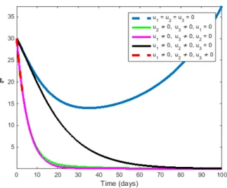
Figure 1 represents the population of infected humans with and without control. The solid blue line denotes the population of infected individuals in system (2.1)-(2.7) without control while the black, pink, orange and red lines denotes the population of infected individuals in system (2.1)-(2.7) using vari-ous combination of the three controls. We see that the population of infected human with control is more sharply decreased than individuals without control. Figure 2represents the total number of rodent population in the system (2.1)-(2.7) with and without control. The solid blue line denotes the total population of rodent in system (2.1)-(2.7) without control while the black, pink, orange and red lines denotes the population of rodent in system (2.1)-(2.7) using various combination of the three controls. We see that the population of rodent with control is more sharply decreased than rodent without control.
5. Concluding Remarks
Figure 1: Simulation showing the effect of u1, u2, u3 only on infec-tious human
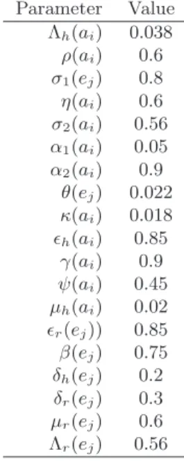
Parameter Value Λh(ai) 0.038
ρ(ai) 0.6
σ1(ej) 0.8
η(ai) 0.6
σ2(ai) 0.56
α1(ai) 0.05
α2(ai) 0.9
θ(ej) 0.022
κ(ai) 0.018
ǫh(ai) 0.85
γ(ai) 0.9
ψ(ai) 0.45
µh(ai) 0.02
ǫr(ej)) 0.85
β(ej) 0.75
δh(ej) 0.2
δr(ej) 0.3
µr(ej) 0.6
Λr(ej) 0.56
Table 1. Description of the model parameters
References
[1] J.B. McCormick, D.H.Walker, I.J. King, P.A. Webb, L.H. Elliott, S.G White, K.M. Johnson, Lassa virus hepatitis: a study of fatal Lassa fever in humans,Am. J. Trop. Med. Hyg.,35(1986), 401-407.
[2] J.D. Frame, J.M. Baldwin, D.J. Gocke, J.M. Troup, Lassa fever a new virus disease of man from West Africa,Am. J. Trop. Med. Hyg.,19(1970), 670-676.
[3] J.D.Frame, J.M. Baldwin, D.J. Gocke, J.M. Troup, Lassa fever a new virus disease of man from West Africa. I: Clinical description and pathological findings,Am. J. Trop. Med. Hyg.,19(1970), 670-676.
[4] D.H. Walker, J.B. Mccormick, K.M. Johnson, P.A. Webb, G. Komba-kano, L.H. Elliott, J,J. Gardner, Pathologic and virologic study of fatal Lassa fever in man,Am. J. Pathol. (1982), 349-356.
[6] P.B. Jahrling, R.A. Hesse, G.A Eddy, K.M. Johnson, R.T. Callis, E.L. Stephen, Lassa virus infection of rhesus monkeys pathogenesis and treat-ment with ribavirin,J. Infect. Dis.(2012), 580-589.
[7] M. Bawa, S. Abdulrahman, O.R. Jimoh, N.U. Adabara, Stability analy-sis of disease free equilibrium state for Lassa fever disease, J. of Science, Technology, Mathematics and Education,9 (2012), 115-123.
[8] R. Okuonghae, D. Okuonghae, A mathematical model for Lassa fever,J. of the Nigeria Association of the Mathematical Physics, 10(2006), 457-464. [9] T.O. James, S. Abdulrahman, S. Akinyemi, N.I. Akinwande, Dynamics
transmission of Lassa fever, International J. of Innovation and Research in Educational Sciences(2012), 2349-5219.
[10] M.O. Onuorah, N.I. Akinwande, M.O. Nasir, M.S. Ojo, Sensitivity analysis of Lassa fever model,International J. of Mathematics and Statistic Studies, 4(2016), 30-49.
[11] N.E. Yun, D.H. Wlker, Pathogenesis of Lassa fever, www.mdpi.com/journal/viruses, 4(1999), 2031-2048.
[12] CDC, Lassa fever Fact Sheet, Available online: http:www.cdc.gov (2012).
[13] W.H. Fleming, R.W. Rishel, Deterministic and Stochastic Optimal Con-trol, Springer, New York (1975).
[14] L.S. Pontryagin , V.T. Boltyanskii, R.V. Gamkrelidze, E.F. Mishcheuko, The Mathematical Theory of Optimal Processes, Class. Sov. Math., Gordon and Breach Science Publishers, New York (1986).
[15] H.R. Joshi, Optimal control of an HIV immunology model,Optimal Control Appl. Math.23(2002), 199-213.
[16] D. Kirschner, S. Lenhart, S. Serbin, Optimal Control of the Chemotherapy of HIV, J. Math. Biol.,35(1997), 775-792.