Step 6 – Buckling/Slenderness Considerations
IntroductionBuckling of slender foundation elements is a common concern among designers and structural engineers. The literature shows that several researchers have addressed buckling of piles and micropiles over the years (Bjerrum 1957, Davisson 1963, Mascardi 1970, Gouvenot 1975). Their results generally support the conclusion that buckling is likely to occur only in soils with very poor strength properties such as peat, very loose sands, and soft clay.
However, it cannot be inferred that buckling of helical screw foundations will never occur. Buckling of helical screw foundations in soil is a complex problem best analyzed using numerical methods on a desktop computer. It involves parameters such as the shaft section and elastic properties, coupling strength and stiffness, soil strength and stiffness, and the eccentricity of the applied load. This section of the design manual presents a summarized description of the procedures available to study the question of buckling of helical screw foundations, and recommendations that aid the systematic performance of buckling analysis.
Background
Buckling of columns most often refers to the allowable compression load for a given unsupported length. The mathematician Leonhard Euler solved the question of critical
compression load in the 18th century with a basic equation included in most strength of
materials textbooks.
Pcrit = π2EI/(KLu)2 (Equation 6.1)
where: E = Modulus of Elasticity
I = Moment of Inertia
K = End Condition Parameter
Lu = Unsupported Length
It is obvious that helical screw foundations have slender shafts - which can lead to very high slenderness ratios (Kl/r), depending on the length of the foundation shaft. This condition would be a concern if the screw foundation were in air or water and subjected to a compressive load. For this case, the critical buckling load could be estimated using the well-known Euler equation above.
However, helical screw foundations are not supported by air or water, but by soil.
This is the reason screw foundations can be loaded in compression well beyond the critical
buckling loads predicted by Equation 6.1. As a practical guideline, soil with
Standard Penetration Test (SPT) blow count per ASTM D-1586 greater than 4 along the entire embedded length of the screw foundation shaft has been found to provide adequate support to resist buckling - provided there are no
horizontal (shear) loads or bending moments applied to the top of the
foundation. Only the very weak soils are of practical concern. For soils with 4 blows/ft or less, buckling calculations can be done by hand using the Davisson (1963) method or by computer solution using the finite-difference technique as implemented in the program
LPILEPLUS (ENSOFT, Austin, TX). In addition, the engineers at Hubbell Power Systems/
Chance have developed a macro-based computer solution using the finite-element
Construction Distributor in your area. Contact information for Hubbell/Chance Civil Construction Distributors can be found at www.abchance.com. These professionals will help you to collect the data required to perform buckling analysis.
Buckling Analysis by Davisson Method
A number of solutions have been developed for various combinations of pile head and tip
boundary conditions and for the cases of constant modulus of subgrade reaction (kh) with
depth. One of these solutions is the Davisson (1963) method as described below. Solutions for various boundary conditions are presented by Davisson in Figure 6.1. the axial load is assumed to be constant in the pile – that is no load transfer due to skin friction occurs and the pile initially is perfectly straight. The solutions shown in Figure 6.1 are in
dimensionless form, as a plot of Ucr versus Imax.
Ucr = PcrR2/EpIp Or Pcr = UcrEpIp/R2 (Equation 6.2)
R = 4√E
pIp/khd (Equation 6.3)
Imax = L/R (Equation 6.4)
where: Pcr= Critical Buckling Load
Ep = Modulus of Elasticity of Foundation Shaft
Ip = Moment of Inertia of Foundation Shaft
kh = Modulus of Subgrade Reaction
d = Foundation Shaft Diameter
L = Foundation Shaft Length over which kh is taken as Constant
Ucr = Dimensionless ratio
Soil Description
Very soft clay Soft clay Loose sand
Table 6.1
Modulus of Subgrade Reaction – Typical Values Modulus of Subgrade
Reaction (kh)
(pci)
15 - 20 30 - 75
20
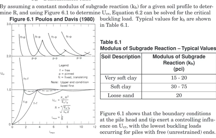
By assuming a constant modulus of subgrade reaction (kh) for a given soil profile to
deter-mine R, and using Figure 6.1 to deterdeter-mine Ucr, Equation 6.2 can be solved for the critical
buckling load. Typical values for kh are shown in Table 6.1.
Figure 6.1 shows that the boundary conditions at the pile head and tip exert a controlling influ-ence on Ucr, with the lowest buckling loads occurring for piles with free (unrestrained) ends.
Design Example 6.1
Determining Critical Buckling Load, Pcr, by Davisson Method
Pcr Model As
h K =15pci Pcr
Foundation
Soft Clay N=3 K =15pcih
Clay N ≥ 5 Stiff
3'
12'
15'
A three-helix Type SS150 11/
2" square shaft helical screw foundation is to be installed into
the soil profile as shown above. The top 3 feet is uncontrolled fill and is assumed to be soft
clay. The majority of the shaft length (12 feet) is confined by soft clay with a kh = 15 pci.
The helix plates will be located in stiff clay below 15 feet. What is the critical buckling load per the Davisson Method?
The buckling model above assumes a pinned-pinned end condition for the pile head and tip. The foundation length is 15 feet, which is the shaft length in the soft clay.
Modulus of Elasticity (Ep) 30 x 106 psi
Moment of Inertia (Ip) 0.396 in4
Shaft Diameter (d)
1.5 in
Physical Properties - Hubbell/Chance Type SS150 Square Shaft Foundations
Assumptions:
1. kh is constant, i.e. it does vary with depth. This is conservative because kh usually does
vary with depth, and in most cases it increases with depth.
2. Pinned-pinned end conditions assumed. In reality, end conditions are more nearly fixed than pinned, thus results are generally conservative.
R = 4√(30 x 106 x 0.396)/(15 x 1.5) = 26.96
Imax = (15 x 12)/26.96 = 6.7
From Figure 6.1, Ucr≈ 2
Another way to determine the buckling load of a helical screw foundation in soil is to model it based on the classical Winkler (a mathematician, circa 1867) concept of a beam-column on an elastic foundation. The finite difference technique can then be used to solve the governing differential equation for successively greater loads until, at or near the buckling load, failure to converge to a solution occurs. The derivation for the differential equation for the beam-column on an elastic foundation was given by Hetenyi (1946). The assumption is made that a shaft on an elastic foundation is subjected not only to lateral loading, but also to compressive force acting at the center of the gravity of the end cross-sections of the shaft, leading to the differential equation:
EI(d4y/dx4) + Q(d2y/dx2) + E
sy = 0 (Equation 6.5)
where: y = lateral deflection of the shaft at a point x along the length of the shaft
x = distance along the axis, i.e. along the shaft EI = flexural rigidity of the foundation shaft
Q = axial compressive load on the helical screw foundation
Esy = soil reaction per unit length
Es = secant modulus of the soil response curve
The first term of the equation corresponds to the equation for beams subject to transverse loading. The second term represents the effect of the axial compressive load. The third term represents the effect of the reaction from the soil. For soil properties varying with depth, it is convenient to solve this equation using numerical procedures such as the finite element or finite difference methods. Reese et al. (1997) outlines the process to solve Equation 6.5 using a finite difference approach. Several computer programs are commercially available that are applicable to piles subject to axial and lateral loads as well as bending moments. Such programs allow the introduction of soil and foundation shaft properties that vary with depth, and can be used advantageously for design of micropiles subject to centered or eccentric loads.
To define the critical load for a particular structure using the finite difference technique, it is necessary to analyze the structure under successively increasing loads. This is
necessary because the solution algorithm becomes unstable at loads above the critical. This instability may be seen as a convergence to a physically illogical configuration or failure to converge to any solution. Since physically illogical configurations are not always easily recognized, it is best to build up a context of correct solutions at low loads with which any new solution can be compared.
Design Example 6.2
Determining Critical Buckling Load by Finite Difference Pcr
5'
50'
Layer 1 FILL N=20, C=0 φ=30°, γ’=48 pcf e50=0, Ks=60 pci
Layer 2 very soft CLAY w/ silt, trace sand N=0, C=15 psf φ=0°, γ’=25 pcf e50=0.06, Ks=10 pci
Layer 3 silty SAND N=30, C=0 φ=35.5°, γ’=58 pcf e50=0, Ks=91pci
A four-helix square shaft helical screw foundation is to be installed into the soil profile as shown above. The top five feet is compacted granular fill and is considered adequate to support lightly
loaded slabs and shallow foundations. The majority of the shaft length (50 feet) is confined by very soft clay described by the borings as “weight of ham-mer” (WOH) or “weight of rod” (WOR) material. WOH or WOR material means the weight of the 130-lb drop hammer or the weight of the drill rod used to extend the sampler down the borehole during the standard penetration test is enough to push the sampler down 18+ inches. As a result, a low cohesion value (15 psf) is assumed. The helix plates will be located in dense sand below 55 feet. What is the critical buckling load of Type SS175 13⁄
4" square shaft and Type HS 31⁄2" pipe shaft
foundations using LPILEPLUS 3.0 for Windows®
(ENSOFT, Austin, TX)?
Once the computer model is completed, the solution becomes an iterative process of applying successively increasing loads until a physically logical solution converges. At or near the critical buckling
load, very small
increasing increments of axial load will result in significant changes in lateral deflection – which is a good indication of elastic buckling. Figure
6.2 is an LPILEPLUS
output plot of lateral shaft deflection vs. depth. As can be seen by the plot, an axial load of 14,561 lb is the critical buckling load for Type SS175 13⁄
4" square shaft because of the dramatic increase in lateral deflection at that load compared to previous lesser loads. Figure 6.3 indicates a critical
buckling load of 69,492 lb for Type HS 31⁄
2" pipe shaft.
Note that over the same 50-foot length of very soft clay, the well-known Euler equation predicts a critical buckling load for Type SS175 of 614 lb with pinned-pinned end
conditions and 2,454 lb with fixed-fixed end conditions. Euler critical buckling load for Type HS is 3,200 lb for pinned-pinned and 12,800 lb for
fixed-fixed. This is a good indication that shaft confinement provided by the soil will significantly increase the buckling load of helical screw foundations. This also indicates that even the softest materials will provide significant resistance to buckling.
Figure 6.2
Plot of Deflection vs. Depth LPILEPLUS Output
All extendable helical screw foundations have couplings or joints - used to connect succeeding sections together in order to install the helix plates in bearing soil. One inherent disadvantage of using the finite difference method is its inability to model the
effects of bolted couplings or joints that have zero joint stiffness until the coupling rotates enough to bring the shaft sides into contact with the coupling walls. This is analogous to saying the coupling or joint acts as a pin connection until it has rotated a specific amount, after which it acts as a rigid element with some flexural stiffness. All bolted couplings or joints, including square shaft and pipe shaft
foundations, have a certain amount of
rotational tolerance. This means the joint initially has no stiffness until it has rotated enough to act as a rigid element. In these cases, it is probably better to conduct buckling analysis using other means, such as finite element analysis, or other methods based on
empirical experience as mentioned earlier. If couplings are
completely rigid, i.e. some flexural stiffness even at zero joint rotation, axial load is transferred without the effects of a pin connection, and the finite difference method can be used. An easy way to accomplish rigid couplings with pipe shaft foundations is to pour concrete or grout down the ID of the pipe after installation. A better method is to install a grout column around the square or pipe shaft of the foundation using the HELICAL
PULLDOWN™ Micropile (HPM) method. The HPM is a patented (U.S. Patent 5,707,180)
installation method initially developed to install helical screw foundations in very weak soils where buckling may be anticipated. The HPM is discussed in the Appendix.
Figure 6.3
Plot of Deflection vs. Depth LPILEPLUS Output
Pcr
Foundation
N = 2 Soft Clay
N = 20 Medium Sand Loose sand
N = 5 12'
30'
A three-helix Type SS5 11/
2" square shaft helical screw
foundation is to be used to underpin an existing
townhouse structure that has experienced settlement. The top 12 feet is loose sand fill, which probably contrib-uted to the settlement problem. The majority of the shaft length (30 feet) is confined by very soft clay with an SPT blow count of 2. As a result, a cohesion value (250 psf) is assumed. The helix plates will be located in me-dium-dense sand below 42 feet. What is the critical buckling load using the ANSYS integrated finite element model?
Hubbell Power Systems/A.B. Chance Company has developed a design tool, integrated
with ANSYS® finite element software, to determine the load response and buckling of
helical screw foundations. The method uses a limited non-linear model of the soil to simulate soil resistance response without increasing solution solve time inherent in a full nonlinear model. The model is still more sophisticated than a simple elastic foundation model, and allows for different soil layers and types.
The screw foundation components are modeled as 3D beam elements assumed to have elastic response. Couplings are modeled from actual test data, which includes an initial zero stiffness, an elastic/rotation stiffness and a final failed condition
– which includes some residual stiffness. Macros are used to create soil property data sets, helical screw foundation component libraries, and load options w/ end conditions at the pile head.
After the helical screw foundation has been configured and the soil and load conditions specified, the macros increment the load, solve for the current load and update the lateral resistance based on the lateral deflection. After each solution, the ANSYS post-processor extracts the lateral deflection and recalculates the lateral stiffness of the soil for each element. The macro then restarts the analysis for the next load increment. This
incremental process continues until buckling occurs. Various output such as deflection and bending moment plots can be generated from the results.
Design Example 6.3 continues, next page Design Example 6.3 Determining Critical Buckling Load by Finite Elements
Figure 6.4
Displaced Shape of Shaft ANSYS® Output
for Design Example 6.3
Output indicates the Type SS5 11/
2" square shaft buckled at around 28 kip. Figure 6.4
shows the displaced shape of the shaft (exaggerated for clarity). The “K0” in Figure 6.4 are the locations of the shaft couplings. Note that the deflection response is controlled by the couplings – as would be expected. Also note that the shaft deflection occurs in the very soft clay above the medium-dense bearing stratum. Since the 28 kip buckling load is considerably less than the bearing capacity (55+ kip) it is recommended to install a grout
column around the 11/
2" square shaft using the HELICAL PULLDOWN™ Micropile (HPM)
method.
1. ASTM D 1586, Standard Test Method for Penetration Test and Split-Barrel Sampling of Soils.
2. Bjerrum, L., 1957, “Norwegian experiences with steel piles to rock,” Geotechnique, Vol.7, 1957.
3. Cadden, Allen and Jesus Gomez, “Buckling of Micropiles,” ADSC-IAF – Micropile Committee, Dallas, TX, 2002.
4. Davisson, M.T., “Estimating Buckling Loads for Piles,” Proceedings, 2nd Pan-American
Conference on Soil Mechanics and Foundation Engineering, Brazil, Vol. 1, 1963. 5. Design Manual, DM7, NAVFAC, Soil Mechanics, Government Printing Office, 1986. 6. HeliCALC Micropile Design Assessment Program – Theoretical and User’s Manual,
Hubbell Power Systems/A.B. Chance Co., 2001.
7. Hetenyi, M., Beams on Elastic Foundation, The University of Michigan Press, Ann Arbor, MI, 1946.
8. Hoyt, Robert M., Gary L. Seider and Lymon C. Reese, and Shin-Tower Wang, “Buckling of Helical Anchors Used for Underpinning,” Proceedings, ASCE National Convention, San Diego, CA, 1995.
9. Reese, L.C., “The Analysis of Piles Under Lateral Loading,” Proceedings, Symposium on the Interaction of Structure and Foundation, Midland Soil Mechanics and Foundation Engineering Society, University of Birmingham, England, 1971.
10. Reese, L.C., W.M Wang, J.A. Arrellaga and J. Hendrix, “Computer program LPILEPLUS