1-s2.0-S0167947317300026-main.pdf

Principal components adjusted variable screening

Zhongkai Liu

a

, Rui Song

a,∗

, Donglin Zeng

b

, Jiajia Zhang

c

a_{Department of Statistics, North Carolina State University, Raleigh, NC, USA} b_{Department of Biostatistics, University of North Carolina at Chapel Hill, NC, USA}

c_{Department of Epidemiology and Biostatistics, University of South Carolina, Columbia, SC, USA}

a r t i c l e i n f o

Article history:

Received 20 March 2016

Received in revised form 29 December 2016 Accepted 31 December 2016

Available online 19 January 2017

Keywords:

Generalized linear models Principal components Variable selection Sure screening

a b s t r a c t

Marginal screening has been established as a fast and effective method for high dimensional variable selection method. There are some drawbacks associated with marginal screening, since the marginal model can be viewed as a model misspecification from the joint true model. A principal components adjusted variable screening method is proposed, which uses top principal components as surrogate covariates to account for the variability of the omitted predictors in generalized linear models. The proposed method is demonstrated with superior numerical performance compared with the competing methods. The effi-ciency of the method is also illustrated with the analysis of the Affymetrix genechip rat genome 230 2.0 array data and the European American SNPs data.

1. Introduction

We consider the problem of ultrahigh dimensional regression, i.e. the dimension of predictors used for predicting a response of interest,p, is much larger than sample size,n. It is often assumed that only a relatively small subset of the predictors contribute to the response. As a result, an efficient method of variable selection, which can identify the most important predictors, plays a key role in the ultra-high dimensional regression.

One group of variable selection methods is based on penalized methods which can select variables and estimate parameters simultaneously through solving an ultrahigh dimensional regression with some pre-specified penalties leading to sparsity. These methods include bridge regression (Frank and Friedman, 1993), LASSO (Tibshirani, 1996), SCAD (Fan and Li, 2001), Dantzig selection (Candes and Tao, 2007), and other folded concave regularization methods (Fan and Lv, 2011;

Zhang and Zhang, 2012). When the dimension is very high, however, these methods may have heavy implementation costs and face challenges in computational feasibility.

Recently, variable screening methods have been re-discovered and advocated in the ultra-high dimensional setting, including sure independence screening (SIS) method (Fan and Lv, 2008), marginal bridge regression based method (Huang et al., 2008) and some others. Specifically, SIS method inFan and Lv (2008) selects important variables in ultrahigh dimensional linear models based on the marginal correlations of each predictor with the response. They showed that the correlation ranking of the predictors possesses a sure independence screening property, that is, the important variables can be selected with probability close to one. Later, the marginal screening method was extended to generalized linear models (Fan and Song, 2010). Various screening methods have been developed, to name a few, tilting methods (Hall et al., 2009), generalized correlation screening (Hall and Miller, 2009), nonparametric screening (Fan et al., 2011), robust rank correlation based screening (Li et al., 2012), and quantile-adaptive model-free feature screening (He et al., 2013).

∗_{Corresponding author.}

E-mailaddress:[email protected](R.Song).

These marginal screening methods face a number of challenges. For example, if the marginal working model is too far away from the true model, it is hard to ensure the sufficient conditions for sure screening to hold. Consequently marginally unimportant but jointly important variables may not be preserved in marginal screening. Meanwhile, the marginal screening methods may include noise variables that are weakly correlated with the important predictors. It can potentially increase false positive rate.

To address these issues, in this paper, we propose a principal component-adjusted screening (PCAS) method for generalized linear models. The key idea is to use principal components as surrogate covariates to account for omitted covariates in marginal screening. Specifically, we fitpmarginal regressions by maximizing the marginal likelihood including not only the screened predictor but also some selected principal components. Then we consider an independence learning by ranking the maximum marginal likelihood estimators or maximum marginal likelihood.

PCAS method has several advantages. First, PCAS retains top principal components as surrogate covariates, thus retains the information in those predictors that are not included in the marginal screening. Second, it possesses good properties of the conditional screening to reduce the correlation among predictors and thus reduce the noise in the process of variable selection. Finally, unlike the conditional sure independence screening method (Barut et al., 2012) where certain variables are known to be responsible for the outcomes, PCAS does not need these prior information of the predictors. Extensive numerical results show that the proposed PCAS method has superior performance to the original SIS method. As an important remark, computing the principal components in the implementation only requires eigenvalue-decomposition of annbynmatrix regardless of the dimensionalityp.

The setup of generalized linear models is introduced in Section2. Section3discussed the computation of principal components. In Section4, we introduced the PCAS procedure with maximum marginal likelihood estimators (MMLE) and marginal likelihood ratio (MLR). Simulation results are presented in Section5and two real data analysis results are illustrated in Section6. Section7gives concluding remarks.

2. Generalized linear models

Consider the generalized linear model where the probability density function of a response variableYtakes the form fY

(

y

;

θ)

=

exp

{

y

θ

−

b

(θ)

+

c

(

y

)

}

, with known functionsb

(

·

)

,c

(

·

)

, and the natural parameter

θ

. Suppose that the observed

data

{

(

Xi

,

Yi

),

i

=

1

, . . . ,

n

}

are identically independent distributed copies of

(

X

,

Y

)

, whereXi

=

(

1

,

Xi1

, . . . ,

Xip

)

T and

Xi1

, . . . ,

Xip arep-dimensional covariates for subjecti.

β

=

(β

0

, β

1

, . . . , β

p

)

T is a

(

p

+

1

)

-vector of parameter. We are

interested in identifying the sparsity structure of

β

from the equation

E

(

Y

|X

=

x

)

=

b′

(θ(

x

))

=

g−1



_p



j=0

β

jxj



,

(1)

wherex

= {

x0

,

x1

, . . . ,

xp

}

Tis a

(

p

+

1

)

-vector withx0

=

1 when considering the intercept,b′

(θ)

is the first order derivative ofb

(θ)

with respect to

θ

andgis the link function. For demonstration purposes, in the paper we only take canonical link function, that isg

=

(

b′

₎

−1_{, into consideration. In this case,}

_θ(

_x

₎

₌



p

j=0

β

jxj. The ordinary linear modelY

=

XT

β

+

ε

, where

ε

is the random error, is a special case of model(1)by using the identity link, i.e.g

(µ)

=

µ

. Considering binary response data, the logistic regression is another special case of model(1)by using the logit linkg

(µ)

=

log

(µ/(

1

−

µ))

.

3. Principal component analysis

Principal component analysis is a widely used tool for high dimensional data analysis in many fields, such as signal processing and dimension reduction. Based on projecting a dataset to another coordinate system by determining the eigenvectors and eigenvalues of the matrix, principal component analysis involves calculations of a covariance matrix of a dataset to minimize the redundancy as well as maximize the variance (Shlens, 2014). A common method to find the eigenvectors and eigenvalues is singular value decomposition (SVD), which decomposes a matrix into a set of rotation and scale matrices. SupposeX

¯

is a matrix withnrows andpcolumns (p

>

n) and columns are normalized to be norm one. A singular value decomposition ofX

¯

is given byX

¯

n×p

= ¯

Un×n

(

diag

(λ

1

, . . . , λ

n

),

0n×₍p−n)

)

V

¯

Tp×p, whereU

¯

andV

¯

are orthonormal

matrices with dimensionsnandprespectively and diag

(λ

1

, . . . , λ

n

)

is a diagonal matrix with diagonal elements

λ

1

, . . . , λ

n.

Additionally,

λ

1

≥

λ

2

≥ · · · ≥

λ

n

≥

0. Since

¯

XTX

¯

= ¯

Vdiag

(λ

2₁

, . . . , λ

2_n

,

0

, . . . ,

0

)

V

¯

T

,

it is clear that the columns ofV

¯

are the principal directions ofX

¯

. Thus, the principal components, that is, the projection ofX’s rows on these directions, should beX

¯

V

¯

= ¯

Un×ndiag

(λ

1

, . . . , λ

n

)

. In other words, each column ofU

¯

represents each principal

component up to some scale.

To calculateU

¯

, we noteX

¯

X

¯

T

_{= ¯}

_Udiag

_(λ

2

1

, . . . , λ

2n

)

U

¯

T. Therefore, if we perform an eigenvalue decomposition onX

¯

X

¯

T,

4. PCAS procedure

LetM⋆

= {

1

≤

j

≤

p

:

β

_j⋆

̸=

0

}

be the true sparse model with non-sparsity sizes

= |

M⋆

|

, where

β

⋆

=

(β

₀⋆

,

β

⋆

1

, . . . , β

p⋆

)

Tdenotes the true value. In this paper, we refer to principal components adjusted models as fitting models with

componentwise covariates and the firstKnprincipal components as offset covariates.

4.1. PCAS with maximum marginal likelihood estimators

PCAS maximum marginal likelihood estimators (PCAS-MMLE)

β

ˆ

M

j , forj

=

1

, . . . ,

p, is defined as the minimizer of the

negative marginal log-likelihood

(

_β

ˆ

M j,0

,

β

ˆ

M j

,

γ

ˆ

M j,1

, . . . ,

γ

ˆ

M j,Kn

)

T

₌

_argmin

β0,βj,γj,1,...,γj,Kn

n



i=1

l



β

0

+

β

jXij

+

Kn



k=1

γ

M

j,kUik

,

Yi



,

forj

=

1

, . . . ,

p

,

wherel

(

Y

;

θ)

= −

(θ

Y

−

b

(θ)

+

c

(

Y

))

, and

{U

k

}

is thekth eigenvector consisting of

{

Uik

}

ni=1.

β

ˆ

M

j measures the strength

of the conditional contribution ofXjgiven the firstKn principal components. These principal components represent the

information of predictors except forXjin the marginal model. The process can be rapidly computed.

Specifically, in ordinary linear models with normality assumption of random errors, the maximum likelihood estimator is identical to the ordinary least squares estimator written as

(

_β

ˆ

M j,0

,

β

ˆ

M j

,

γ

ˆ

M j,1

, . . . ,

γ

ˆ

M j,Kn

)

T

₌

_argmin

β0,βj,γj,1,...,γj,Kn

n



i=1



Yi

−

β

0

−

β

jXij

−

Kn



k=1

γ

M

j,kUik



2

,

forj

=

1

, . . . ,

p

.

We select a set of variables



Mγn

= {

1

≤

j

≤

p

: | ˆ

β

M

j

| ≥

γ

n

}

,

(2)

where

γ

n is a given threshold value. By ranking the importance of features according to their magnitude of marginal

regression coefficients adjusted for a proportion of principal components, we retain variables with large conditional contribution given these principal components. Such an independence learning helps to decrease the dimension of the parameter space fromp(possibly hundreds of thousands) to a much smaller number by choosing a large

γ

n, leading to a

more feasible computation. Although interpretations and implications of principal components adjusted models are still biased from the joint model, the non-sparse information about the joint model can be passed along to the marginal model under a mild condition. Hence it is suitable for the purpose of variable screening.

Since the rationale to use the principal components as surrogate covariates is to account for the effect of the omitted covariates in the marginal model, we should compute the principal components based on thep

−

1 omitted covariates for each marginal regression. For simplicity of computation, we compute the principal components based on allpcovariates and use these principal components as surrogate covariates. Based on our observations, the numerical performance of two methods are very close while the latter one has significantly smaller computational costs.

4.2. PCAS with marginal likelihood ratio

As an alternative method, we can also rank variables based on the likelihood reduction of the variableXjgiven the first

Knprincipal components, which we call PCAS with maximum likelihood ratio (PCAS-MLR):

Lj,n

=

Pn



l



ˆ

β

M

j Xj

+

Kn



k=1

ˆ

γ

M

j,kUk

,

Y



−

_Pn

{

l

(

β

ˆ

₀M

,

Y

)

}

,

forj

=

1

, . . . ,

p

,

where _Pnf

(

X

,

Y

)

=

n−1



n

i=1f

(

Xi

,

Yi

)

is the empirical measure, and

β

ˆ

0M

=

argmin

β0 Pnl

(β

0

,

Y

)

. Denote Ln

=

(

L1,n

,

L2,n

, . . . ,

Lp,n

)

T. Specifically, in ordinary linear models,

Lj,n

=

n



i=1



Yi

− ˆ

β

jMXij

−

Kn



k=1

ˆ

γ

M

j,kUik



2

−

n



i=1

(

Yi

− ˆ

β

0M

)

2

_,

forj

=

1

, . . . ,

p

,

where

_β

ˆ

M

0

=

argmin β0



n

i=1

(

Yi

−

β

0

)

2.

The smaller theLj,nis, the more the variableXjcontributes. We sort the vectorLn in an ascending order and choose

variables according to



Nνn

= {

1

≤

j

≤

p

:

Lj,n

≤

ν

n

}

,

(3)

where

ν

nis a predefined thresholding parameter. PCAS-MLR ranks the importance of features according to their marginal

4.3. Determining the number of selected variables

It remains open on how to choose the number of selected variablesdin variable screening literature. In applications, it is common for practitioners to select a fixed number of top-ranked variables, as the fixed number may reflect prior knowledge of the number of susceptible predictors or budget limitations. Another commonly used procedure is to set the size of the selected set to a number less than the sample size, for exampled

= [

2n

/

log

(

n

)

]

(Fan and Lv, 2008), so that the follow-up analysis can be performed in ap

<

nscenario. Data-driven procedures for determining the size of the important set are appealing but relatively limited. They include information criteria, such as AIC and BIC, and the false discovery rate (FDR) based methods (Barut et al.,2012;Zhao and Li, 2012). These methods, however, have large computational cost, especially in the ultra-high dimensional framework. FollowingFan and Lv(2008), we usedd

= [

2n

/

log

(

n

)

]

in this paper.

4.4. Determining the number of principal components

The choice of numbers of principal componentsKnis critical for PCAS. We propose to use the following two data adaptive

methods. The first method is the scree plot, a classical method in factor analysis to determine the number of principal components. As a related numerical method, we can also use the maximum eigenvalue ratio criterion (Luo et al., 2009), defined as

λ

j

/λ

j+1with 1

≤

j

≤

n

−

1 and

λ

1

≥

λ

2

≥ · · · ≥

λ

n

>

0. We choose the number of principal components that

can maximize the eigenvalue ratio, that is,

ˆ

k

=

argmax 1≤j≤kmax

(λ

j

/λ

j+1

),

(4)

wherekmax

≤

nis a prespecified maximum factor dimension. When the predictors’ correlation structure follows a factor model, it was shown inWang(2012) thatk

ˆ

is consistent to the dimension of the linear subspace spanned by the column vectors of factors’ matrix.

5. Simulations

In this section, we present several simulated linear model examples and logistic regression model examples to evaluate the performance of the proposed procedure and to demonstrate some factors influencing the false selection rate. We implement four different scenarios to generate data. We vary the size of the nonsparse set of coefficients as well as the number of principal components from 1 to 100 for different scenarios, to gauge difficulties of simulation models on the basis of 200 simulations with sample size 500.

For each simulation setting, we apply two marginal sure independence screening (SIS) procedures based on marginal maximum likelihood estimator (MMLE) and marginal likelihood ratio (MLR), and two PCAS procedures including PCAS-MLR and PCAS-MMLE, to screen variables. The minimum model size required for each method to have a sure screening, i.e. to contain the true modelM_⋆, is used as a measure of the effectiveness of a screening method. This avoids the issues of choosing the thresholding parameter. For each simulation model, we evaluate each method by summarizing the median minimum model size (MMMS) as well as its robust estimate of the standard deviation (RSD), which is the associated interquartile range (IQR) divided by 1.34.

5.1. Simulation model I

The covariatesX

=

(

X1

, . . . ,

Xp

)

T are generated from a multivariate normal distribution with mean vector0 and

compound symmetric covariance matrixΣ, where

ρ

=

Σ_ij

=

0

.

4, wheni

̸=

j. The size of the non-sparse set sizesis taken as 6, 8 and 12 with the true regression coefficients recorded inTable 1. The MMMS of selected models with its associated RSD for linear models and logistic regression models withp

=

1000 andp

=

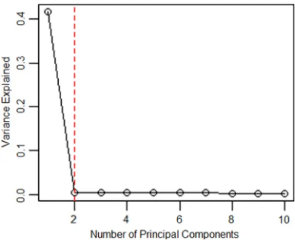
10 000 are shown inTable 1. We record the results of PCAS with number of PCs taking as 1, 3, 5, 10, 30, 50 and 100 respectively. The case of zero PCs is SIS method (Fan and Song, 2010). The scree plot is provided asFig. 1.

Since the first principal component can explain over 40% of the total variability in the observed covariate matrix, much larger than that of the rest PCs, the scree plot inFig. 1suggests that the number of PCs taken should be one. In addition, the maximum eigenvalue ratio estimator gives the same choice, i.e.k

ˆ

=

1. This is consistent with our observation inTable 1, where PCAS performs the best when only one PC is adjusted. The performance of PCAS method is not improved with the increase in the number of principal components. It is reasonable since the proportion of the variation that can be explained by the rest of PCs is so small that including more PCs will not be helpful to account for the additional contribution from the rest of the covariates, instead, it leads to larger estimation variation hence deteriorates the performance of PCAS. We also compute the cases for

ρ

=

0

.

2

,

0

.

6 and 0.8. Since the results demonstrate a similar trend, we omit the details.

5.2. Simulation model II

Table 1

The MMMS and RSD (in parenthesis) of the simulated examples for linear and logistic regression from simulation model I withn=500 whenp=1000 andp=10 000. PC=0 refers to the marginal screening inFan and Lv(2008).

PCs Variance SIS-PCA-MLR SIS-PCA-MMLE SIS-PCA-MLR SIS-PCA-MMLE

Setting 1, linear model withp=1000

s=6,β⋆=(0.3,−0.3,0.3, . . .)T _s=12,β⋆_{=(3,4,3, . . .)}T

0 0 13(35) 13(35) 101(96) 101(96)

1 41.5% 7(3) 7(4) 12(0) 12(0)

3 42.2% 7(3) 7(4) 12(0) 12(0)

5 42.8% 7(3) 7(3) 12(0) 12(0)

10 44.4% 7(4) 7(4) 12(0) 12(0)

30 50.2% 8(5) 8(5) 12(0) 12(0)

50 55.4% 11(8) 10(8) 12(0) 12(0)

100 66.4% 19.5(32) 19(31) 12(1) 12(1)

Setting 2, logistic regression withp=1000

s=6,β⋆=(0.7,−0.7,0.7, . . .)T _s=8,β⋆_{=(3,4,3, . . .)}T

0 0 14(26) 14(26) 70.5(80) 64(82)

1 41.7% 7(3) 7(3) 21(31) 23(28)

3 42.4% 7(3) 7(3) 22.5(31) 24(30)

5 43.0% 7(4) 7(3) 25(29) 26(32)

10 44.6% 7(4) 8(4) 24(38) 27(38)

30 50.4% 8(7) 8(7) 38(49) 37(46)

50 55.5% 10(10) 10.5(10) 58(72) 60(80)

100 66.5% 22(34) 24.5(34) 532(460) 414(347)

Setting 3, linear model withp=10 000

s=6,β⋆=(0.3,−0.3,0.3, . . .)T _s=12,β⋆_{=(3,4,3,4, . . .)}T

0 0 90.5(501) 90.5(501) 830.5(924) 830.5(924)

1 40.3% 14.5(37) 14(35) 12(1) 12(1)

3 40.6% 15(35) 14(34) 12(1) 12(1)

5 41.0% 15(30) 14(29) 12(1) 12(1)

10 41.9% 16.5(36) 15(35) 12(1) 12(1)

30 45.2% 27(49) 25.5(45) 12(1) 12(1)

50 48.5% 36.5(100) 36.5(95) 12(2) 12(2)

100 56.1% 70.5(171) 67.5(170) 14(8) 14(7)

Setting 4, logistic regression withp=10 000

s=6,β⋆=(0.7,−0.7,0.7, . . .)T _s=8,β⋆_{=(3,4,3, . . .)}T

0 0 112(365) 112(366) 641(742) 609.5(731)

1 41.5% 15(30) 16(29) 142(339) 146(354)

3 41.8% 16(32) 17(32) 149.5(372) 160(351)

5 42.2% 15(37) 17(36) 157(392) 168.5(394)

10 43.0% 16.5(35) 17(37) 154(351) 160(367)

30 46.3% 28(51) 26(50) 259(663) 259(646)

50 49.5% 36(68) 34.5(71) 410.5(834) 455(879)

100 57.0% 78.5(206) 80.5(238) 6837(6317) 2570(3513)

Table 2

The MMMS and RSD (in parenthesis) of the simulated examples for linear and logistic regression model II using different number of PCs withn=500

whenp=1000 andp=10 000.

PCs Variance SIS-PCA-MLR SIS-PCA-MMLE SIS-PCA-MLR SIS-PCA-MMLE

Setting 1, linear model withp=1000

s=6,β⋆=(0.3,−0.3,0.3, . . .)T _s=12,β⋆_{=(3,4,3,4, . . .)}T

0 0 12(35) 12(35) 30(21) 30(21)

1 18.4% 14(37) 84(66) 30.5(21) 31.5(23)

3 45.3% 19.5(32) 177.5(88) 30(19) 34.5(28)

5 63.6% 7(2) 53(26) 12(0) 39(16)

10 64.8% 7(3) 54(28) 12(1) 38(18)

30 68.9% 9(10) 63.5(40) 12(1) 35(15)

50 72.5% 14(15) 72(51) 12(1) 30.5(15)

100 79.8% 52.5(75) 119(109) 13(2) 28(15)

Setting 2, logistic regression withp=1000

s=6,β⋆=(0.7,−0.7,0.7, . . .)T _s=12,β⋆_{=(−3,4,−3,4, . . .)}T

0 0 13(37) 13(37) 856.5(241) 856.5(241)

1 18.7% 14.5(39) 81(73) 862(216) 879(193)

3 46.8% 19(37) 171(90) 878.5(165) 922.5(111)

5 64.7% 7(3) 50(26) 14(5) 73(35)

10 65.8% 7(3) 51(30) 15(7) 76(40)

30 69.9% 9(8) 59(39) 19(16) 84(49)

50 73.4% 12(15) 66(49) 25.5(33) 97(63)

100 80.6% 58(96) 132.5(127) 67(79) 139(98)

Setting 3, linear model withp=10 000

s=6,β⋆=(0.3,−0.3,0.3, . . .)T _s=12,β⋆_{=(3,4,3,4, . . .)}T

0 0 126.5(381) 126.5(381) 165.5(190) 165.5(190)

1 18.4% 154(357) 831(705) 168(186) 190(226)

3 46.8% 190.5(316) 1832.5(734) 154.5(186) 255(330)

5 64.6% 16(22) 489(242) 12(1) 179(113)

10 65.2% 16(29) 490(289) 12(1) 201(109)

30 67.3% 21.5(48) 549(325) 12(1) 206(118)

50 69.3% 34.5(74) 646(392) 12(2) 238(122)

100 74.0% 105(184) 860(590) 14(6) 284.5(162)

Setting 4, logistic regression withp=10 000

s=6,β⋆=(0.7,−0.7,0.7, . . .)T _s=12,β⋆_{=(−3,4,−3,4, . . .)}T

0 0 163.5(302) 163.5(302) 7978.5(2840) 7978.5(2840)

1 2.0% 160(307) 240.5(327) 8122(2625) 8147.5(2583)

3 5.3% 167.5(300) 312(336) 8039.5(2382) 8092(2325)

5 7.4% 15(26) 51(29) 39(63) 77(40)

10 8.8% 15.5(27) 52(31) 41.5(57) 78.5(39)

30 14.1% 21(45) 56.5(36) 50(91) 85.5(46)

50 19.3% 30(65) 65.5(42) 71(118) 95(61)

100 31.3% 57(125) 87(65) 139(244) 128.5(127)

The MMMS of the selected models with its associated RSD for linear models and logistic regression models withp

=

1000 andp

=

10 000 are shown inTable 2.

PCAS-MLR seems to outperform PCAS-MMLE in terms of smaller MMMS and RSD in many cases. Unlike PCAS-MMLE which uses only the information of magnitudes of estimators, PCAS-MLR makes use of more information, including the magnitudes of the estimators as well as their associated variation.

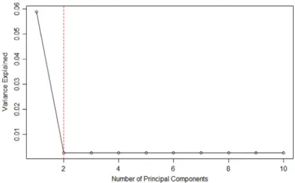
The scree plot inFig. 2suggests to choose five principal components based on the variance explained. In addition, the maximum eigenvalue ratio estimator gives the same answer, i.e.k

ˆ

=

5. It is obvious that PCAS method with five principal components adjusted outperforms SIS, and the performance of PCAS method is highly related to the number of PCs used.

5.3. Simulation model III

This simulation model is adopted from Shen and Huang(2008), where variables are generated after creating the covariance matrix. First, we generate vectors

v

i

,

i

=

1

, . . . ,

p, according to a standard normal distribution and let

V

=

(v

₁

, . . . , v

_p

)

′_{. LetCbe a diagonal matrix, where among the diagonal entries, the top five values are set as 50 and the}

rest are randomly drawn from a standard uniform distribution. In this way we can generate covariates from a multivariate normal distribution with mean0and covariance matrixΣ

=

VCVT_{. The MMMS of the selected models with its associated}

RSD for linear models and logistic regression models withp

=

1000 andp

=

10 000 are shown inTable 3. The scree plot in

Fig. 2. The scree plot for linear models in simulation model II withp=1000 andn=500.

Table 3

The MMMS and RSD (in parenthesis) of the simulated examples for linear and logistic regression model III using different number of PCs withn=500

whenp=1000 andp=10 000.

PCs Variance SIS-PCA-MLR SIS-PCA-MMLE SIS-PCA-MLR SIS-PCA-MMLE

Setting 1, linear model withp=1000

s=6,β⋆=(3,−3,3,−3, . . .)T _s=12,β⋆_{=(3,4,3,4, . . .)}T

0 0 29(20) 29(20) 802.5(121) 802.5(121)

1 7.5% 157.5(173) 135.5(153) 808(229) 813.5(222)

2 14.0% 90.5(150) 50.5(120) 669.5(291) 685(284)

3 20.0% 56.5(161) 26(95) 369(372) 378.5(367)

5 30.8% 6(0) 6(0) 16(6) 15(7)

10 34.0% 6(0) 6(0) 15(6) 14.5(4)

30 44.7% 6(0) 6(0) 14.5(6) 14(6)

50 53.3% 6(0) 6(0) 14(4) 14(6)

100 69.3% 6(0) 6(0) 14(4) 15(5)

Setting 2, logistic regression withp=1000

s=6,β⋆=(3,−3,3,−3, . . .)T _s=8,β⋆_{=(1.3,1,1.3,1, . . .)}T

0 0 43.5(34) 44(35) 333.5(124) 333.5(124)

1 6.9% 24(35) 24(32) 378.5(190) 613(336)

2 13.6% 18.5(19) 18(18) 364(164) 387(151)

3 19.7% 11.5(13) 9.5(10) 291(247) 272.5(237)

5 30.8% 6(0) 6(0) 8(0) 8(0)

10 34.0% 6(0) 6(0) 8(0) 8(1)

30 44.7% 6(0) 6(0) 8(0) 8(0)

50 53.3% 6(0) 6(0) 8(0) 8(0)

100 69.2% 7(4) 8(4) 8(0) 8(1)

Setting 3, linear model withp=10 000

s=6,β⋆=(0.2,−0.2,0.2, . . .)T _s=12,β⋆_{=(3,4,3,4, . . .)}T

0 0 98(117) 98(117) 142.5(291) 142.5(291)

1 2.1% 111(126) 106(135) 62(134) 65(142)

2 4.2% 87.5(149) 92(161) 19(72) 21(58)

3 6.2% 60(120) 54.5(123) 15(9) 15.5(11)

5 9.8% 58(127) 52(141) 12(2) 12(3)

10 11.4% 54(106) 53.5(110) 12.5(2) 13(3)

30 17.5% 73.5(152) 96.5(180) 12(3) 13(5)

50 23.3% 90(235) 101(204) 13(2) 13(3)

100 36.3% 261(383) 282.5(395) 14(13) 15(17)

Setting 4, logistic regression withp=10 000

s=6,β⋆=(0.5,−0.5,0.5,−0.5, . . .)T _s=8,β⋆_{=(1.3,1,1.3,1, . . .)}T

0 0 48(118) 48(118) 13(26) 13(26)

1 1.3% 42.5(110) 43(106) 13(22) 13(26)

3 3.6% 40.5(95) 44(88) 12.5(13) 13(14)

5 5.6% 38.5(73) 40(78) 11(11) 11(12)

10 7.3% 44(74) 46(84) 11(9) 12(11)

30 13.7% 61(120) 60(131) 12(17) 13(21)

50 19.7% 94.5(181) 95.5(178) 15.5(25) 16(28)

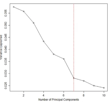
Fig. 3. The scree plot for linear models in simulation model III withp=1000 andn=500.

Table 4

The MMMS and RSD (in parenthesis) of the simulated examples for linear model IV using different number of PCs withs=12,β⋆=(1,1.3,1,1.3,1,1.3, . . .)T_{whenp=40 000 andn=500.}

PCs Variance SIS-PCA-MLR SIS-PCA-MMLE

(SIS-MLR) (SIS-MMLE)

0 0 39(70) 39(70)

1 5.9% 13(4) 13(3)

3 6.3% 13(4) 13(4)

5 6.8% 13(4) 13(4)

10 8.0% 13(4) 13(4)

30 12.2% 14(6) 14(7)

50 17.0% 15(12) 15.5(11)

100 27.8% 23(35) 22(37)

5.4. Simulation model IV

This simulation study imitates a genome-wide analysis where the covariates represent genotype status at each SNP across the whole genome. Furthermore, the correlation among all SNPs carries subject’s ancestry information reflection latent population substructures which should be controlled when assessing each SNP effect. The covariatesX

=

(

X1

, . . . ,

Xp

)

T

is generated according to the Balding–Nichols model (Balding and Nichols, 1995) as follows. First, we generate a latent variableY∗_{that follows a Bernoulli distribution with parameter 0.5. Second, we generate covariatesXfrom a multinomial} distribution with parameters depending on the value of the latent variableY∗. If Y∗

=

0, X follows a multinomial distribution with parameters

(

n

, (

1

−

pl

)

2

,

2pl

(

1

−

pl

),

p2l

)

. If Y

∗

₌

_{1, X follows a multinomial distribution with}

(

n

,

(1−pl)2

(1−pl)2+2Rpl(1−pl)+R2p2l

,

2Rpl(1−pl) (1−pl)2+2Rpl(1−pl)+R2p2l

,

R2_p2 l

(1−pl)2+2Rpl(1−pl)+R2p2l

)

as the parameters, whereplfollows a Beta distribution

with shape parameters p(1−FST)

FST and

(1−p)(1−FST)

FST . In addition,FST

=

0

.

04 represents the genetic distance between two populations,p

=

0

.

5, and the relative riskR

=

0

.

5. We considers

=

3

,

6 and 12 for different levels of sparsity. When s

=

3,

β

∗

=

(

1

,

1

.

3

,

1

)

T. Whens

=

6,

β

∗

=

(

3

,

−

3

,

3

,

−

3

,

3

,

−

3

)

T. Whens

=

12,

β

⋆

=

(

1

,

1

.

3

,

1

,

1

.

3

,

1

,

1

.

3

, . . .)

T. The MMMS of the selected models with its associated RSD for linear models whens

=

12 are shown inTable 4.

PCAS and SIS can both perfectly identify important predictors whens

=

3 or 6, therefore the results are not shown in the table format. This may be because the independence structure among predictors leads to the equivalence between the joint population signal and the marginal population signal. We now discuss the case whens

=

6. Based on the above simulation model, we generate i.i.d. random variablesX1

, . . . ,

Xp,E

(

XiXj

)

=

E

(

Xi

)

E

(

Xj

)

=

0 fori

̸=

jandE

(

Xj2

)

=

1. Whenj

≤

s

=

6,

EXjY

=

EXj

(



s

k=1

β

kXk

+

ϵ)

=

3 or

−

3. Whenj

>

s

=

6, because of the independence structure,EXjY

=

0. It is similar for

s

=

3 case. Although still being a model misspecification, the sparsity structure of the joint model is the same as that of the marginal model. Moreover, there is a clear gap between the marginal signal and the marginal noise. As a result, we can pick up the exact number of important variables with both PCAS and SIS.

Fig. 4. Scree plot for linear models in simulation model IV withp=40 000 andn=500.

Table 5

Comparison between SIS and PCA-SIS over the rats testing data.

Method Prediction error Standard deviation

SIS 0.4636 0.2563

PCA-SIS 0.2278 0.08762

6. Real data analysis

6.1. Affymetric GeneChip Rat Genome 230 2.0 Array example

To illustrate the proposed method, we analyze the dataset reported inScheetz et al.(2006), where 120 12-week-old male rats were selected for harvesting of tissue from the eyes and subsequent microarray analysis. The microarrays used to analyze the RNA from the eyes of these animals contain more than 31,042 different probe sets (Affymetric GeneChip Rat Genome 230 2.0 Array). The intensity values were normalized using the robust multichip averaging method (Irizarry et al., 2003) to obtain summary expression values for each probe set. Gene expression levels were analyzed on a logarithmic scale. We are interested in finding the genes that are related to the TRIM32 gene, which was found to cause Bardet-Biedl syndrome (Chiang et al., 2006) and is a genetically heterogeneous disease of multiple organ systems, including the retina. Although more than 30,000 probe sets are represented on the Rat Genome 230 2.0 Array, many of these are not expressed in the eye tissue. We focus only on the 18,975 probes that are expressed in the eye tissue.

We apply SIS and the proposed PCAS to this dataset, wheren

=

120 andp

=

18

,

975. Because the performance of PCAS-MLR is no worse than that of PCAS-MMLE, we only present the results from PCAS-PCAS-MLR. With PCAS-PCAS-MLR, we choose the first 2 principal components based on its scree plot shown inFig. 5as well as the maximum eigenvalue ratio estimatork

ˆ

=

2.

To evaluate the accuracy of two methods, we use cross validation and compare the prediction error (PE):

PE

=

1

n

n



i=1

(

yi

− ˆ

yi

)

2

,

whereyiis the observed value andy

ˆ

iis the predicted value. By 6-fold cross validation, we randomly partition the data into a

training data set of 100 observations and a testing set of 20 observations. On the training data set, we conduct each variable screening method to selectd

=

50 variables, following the suggestion inFan and Lv(2008). Based on these selected variables, we obtain the ordinary least squares (OLS) estimates of the coefficients in the linear regression model, and make a prediction on the testing data set. Then we compare the predicted response with the true response, and obtain the prediction error as well as its standard deviation. As shown inTable 5, PCAS-MLR gives the prediction error 0.2278, which is about 50% smaller than 0.4636 produced by SIS. Furthermore, the much smaller standard deviation of PCAS-MLR indicates that PCAS-MLR is more robust than SIS method in this data analysis.

6.2. European American SNP example

Fig. 5. Scree plot for Rat Genome data withp=18 975 andn=120.

Fig. 6. Scree plot for SNP data withp=277 andn=360.

(2006), we use 360 observations after removing outlier individuals. We are interested in finding the SNPs that are related to the height phenotype (0/1 binary data) in European Americans, which leads to 277 variables (Price et al., 2006). We implement the proposed method and the marginal screening method on the data set, wheren

=

360 andp

=

277. Both the scree plot inFig. 6and the maximum eigenvalue ratio estimatork

ˆ

=

6 suggest to use 6 principal components.

Similar as before, we implement 6-fold cross validation to partition the data into a training data set of 300 observations and a testing set of 60 observations. On the training data set, we selectd

= [

2n

/

log

(

n

)

]

variables using each variable screening method, and fit the logistic regression based on these selected variables. We then make a prediction on the testing data set, and evaluate the prediction effect by the area under ROC curve (AUC). The result shows that PCAS-MLR obtains a 9.42% larger AUC value than that of SIS and a relatively smaller standard deviation, indicating that PCAS-MLR is preferred in terms of accuracy and robustness.

7. Concluding remarks

the accuracy as well as the robustness of estimation when dimensionality is ultrahigh. Our proposed method shows improvement from both simulation and real data analysis results.

It is important yet challenging to decide how many principal components should be used when performing this method. In the paper, we use maximum eigenvalue ratio estimator along with the scree plot. There are a few challenges in theoretical development. First, to achieve model selection consistency, it is critical to establish that the marginal signals can preserve the sparsity structure of the joint signals. Given that the firstKnprincipal components are adjusted, it is challenging to derive

the population marginal signals and their sparsity structure. Second, ideally we should use the principal components based on thep

−

1 omitted covariates for each marginal variableXj, but it will be computationally intensive hence we recommend

to compute the principal components based on allpcovariates and use them as surrogate covariates for all the marginal variables. Although this approach greatly reduces the computation costs and has almost the same numerical performance, it brings additional challenges in theoretical development since the contribution of each marginal variable is somehow overly counted in the calculation of the principal components. These are interesting topics for future research.

Software

Software in the form of R code, together with input data sets and complete documentation is available on request from the corresponding author ([email protected]).

Acknowledgments

The authors would like to thank two anonymous reviewers whose comments greatly helped improve the quality of the manuscript. Rui Song’s research is partially supported by the NSF grant DMS-1555244 and NCI grant P01 CA142538. Donglin Zeng’s research is partially supported by NIH grants U01-NS082062 and R01GM047845.

References

Balding, D.J., Nichols, R.A.,1995. A method for quantifying differentiation between populations at multi-allelic loci and its implications for investigating identity and paternity. Genetica 96 (1–2), 3–12.

Barut, E., Fan, J., Verhasselt, A., 2012. Conditional sure independence screening. arXiv preprintarXiv:1206.1024. Candes, E., Tao, T.,2007. The dantzig selector: statistical estimation when p is much larger than n. Ann. Statist. 2313–2351.

Chiang, A.P., Beck, J.S., Yen, H.-J., Tayeh, M.K., Scheetz, T.E., Swiderski, R.E., Nishimura, D.Y., Braun, T.A., Kim, K.-Y.A., Huang, J., et al.,2006. Homozygosity mapping with snp arrays identifies trim32, an e3 ubiquitin ligase, as a bardet–biedl syndrome gene (bbs11). Proc. Natl. Acad. Sci. 103 (16), 6287–6292. Fan, J., Feng, Y., Song, R.,2011. Nonparametric independence screening in sparse ultra-high-dimensional additive models. J. Amer. Statist. Assoc. 106 (494). Fan, J., Li, R.,2001. Variable selection via nonconcave penalized likelihood and its oracle properties. J. Amer. Statist. Assoc. 96 (456), 1348–1360. Fan, J., Lv, J.,2008. Sure independence screening for ultrahigh dimensional feature space. J. R. Stat. Soc. Ser. B Stat. Methodol. 70 (5), 849–911. Fan, J., Lv, J.,2011. Nonconcave penalized likelihood with np-dimensionality. IEEE Trans. Inform. Theory 57 (8), 5467–5484.

Fan, J., Song, R.,2010. Sure independence screening in generalized linear models with np-dimensionality. Ann. Statist. 38 (6), 3567–3604. Frank, L.E., Friedman, J.H.,1993. A statistical view of some chemometrics regression tools. Technometrics 35 (2), 109–135.

Hall, P., Miller, H.,2009. Using generalized correlation to effect variable selection in very high dimensional problems. J. Comput. Graph. Statist. 18 (3). Hall, P., Titterington, D., Xue, J.-H.,2009. Tilting methods for assessing the influence of components in a classifier. J. R. Stat. Soc. Ser. B Stat. Methodol. 71

(4), 783–803.

He, X., Wang, L., Hong, H.G.,2013. Quantile-adaptive model-free variable screening for high-dimensional heterogeneous data. Ann. Statist. 41 (1), 342–369. Huang, J., Horowitz, J.L., Ma, S.,2008. Asymptotic properties of bridge estimators in sparse high-dimensional regression models. Ann. Statist. 36 (2),

587–613.

Irizarry, R.A., Hobbs, B., Collin, F., Beazer-Barclay, Y.D., Antonellis, K.J., Scherf, U., Speed, T.P.,2003. Exploration, normalization, and summaries of high density oligonucleotide array probe level data. Biostatistics 4 (2), 249–264.

Li, G., Peng, H., Zhang, J., Zhu, L.,2012. Robust rank correlation based screening. Ann. Statist. 40 (3), 1846–1877. Luo, R., Wang, H., Tsai, C.-L.,2009. Contour projected dimension reduction. Ann. Statist. 37 (6B), 3743–3778.

Price, A.L., Patterson, N.J., Plenge, R.M., Weinblatt, M.E., Shadick, N.A., Reich, D.,2006. Principal components analysis corrects for stratification in genome-wide association studies. Nature Genet. 38 (8), 904–909.

Scheetz, T.E., Kim, K.-Y.A., Swiderski, R.E., Philp, A.R., Braun, T.A., Knudtson, K.L., Dorrance, A.M., DiBona, G.F., Huang, J., Casavant, T.L.,2006. Regulation of gene expression in the mammalian eye and its relevance to eye disease. Proc. Natl. Acad. Sci. 103 (39), 14429–14434.

Shen, H., Huang, J.Z.,2008. Sparse principal component analysis via regularized low rank matrix approximation. J. Multivariate Anal. 99 (6), 1015–1034. Shlens, J., 2014. A tutorial on principal component analysis. arXiv preprintarXiv:1404.1100.

Tibshirani, R.,1996. Regression shrinkage and selection via the lasso. J. R. Stat. Soc. Ser. B Stat. Methodol. 267–288. Wang, H.,2012. Factor profiled sure independence screening. Biometrika 99 (1), 15–28.

Zhang, C.-H., Zhang, T.,2012. A general theory of concave regularization for high-dimensional sparse estimation problems. Statist. Sci. 27 (4), 576–593. Zhao, S.D., Li, Y.,2012. Principled sure independence screening for Cox models with ultra-high-dimensional covariates. J. Multivariate Anal. 105 (1),