HIGHER-ORDER EFFECTS IN CONDENSED PHASE SPECTROSCOPY AND DYNAMICS
Thomas Paul Cheshire
A dissertation submitted to the faculty at the University of North Carolina at Chapel Hill in partial fulfillment of the requirements for the degree of Doctor of Philosophy in the Department
of Chemistry.
Chapel Hill 2018
© 2018
ABSTRACT
Thomas Paul Cheshire: Higher-Order Effects in Condensed Phase Spectroscopy and Dynamics (Under the direction of Andrew M. Moran)
Researchers in the 1970s wondered whether traditional Raman experiments could distinguish homogeneous and inhomogeneous line broadening mechanisms. Since then, a
feedback between experiment and theory has spawned and matured the field of multidimensional Raman spectroscopy and laid the groundwork for modeling nonlinear photoinduced reaction pathways. Here two-dimensional resonance Raman (2DRR) spectroscopy is developed to
investigate photochemical reaction mechanisms and structural heterogeneity in condensed phase systems. Models are developed to understand 2DRR spectra and extended to incorporate non-radiative transitions.
The photodissociation reaction of triiodide serves to uncover the capabilities of 2DRR. A unique pattern of 2DRR resonances is associated with the transition of a nuclear wavepacket from reactant to product. The pattern of resonances is reproduced by modeling the
2DRR spectroscopy is further used to investigate oxygen- and water-ligated myoglobin line broadening mechanisms. Vibrational modes proximal to propionic acid side chains of the heme exhibit significant heterogeneity in the 2DRR spectra. A hydrophobic pocket encompasses the heme, but the side chains are exposed to solvent. Molecular dynamics (MD) simulations suggest that fluctuations in the side chain geometries are correlated with the heterogeneity. 2DRR spectra and MD simulations reveal that the side chains function as effective pathways for thermal relaxation.
Despite progress, a major challenge still plagues multidimensional Raman spectroscopy. Cascading signals radiated in the same direction as the desired signal can render a signal
ACKNOWLEDGEMENTS
I would like to express my sincerest gratitude for my research advisor, Dr. Andrew Moran. His resolute guidance has steered me true during my graduate studies. This spirit of mentorship has been passed along to former and present members of his research team, of which I am truly thankful. Dr. Paul Giokas and Dr. Brian Molesky were instrumental to my initiation and maturation in the field of nonlinear spectroscopy. And finally, the work in this dissertation was done in parallel with that of Dr. Zhenkun Guo, to whom I would like to extend my
TABLE OF CONTENTS
LIST OF TABLES ... xiii
LIST OF FIGURES ... xiv
LIST OF ABBREVIATIONS ... xxxii
LIST OF SYMBOLS ... xxxiv
CHAPTER I: INTRODUCTION ... 1
I. Overview ... 1
II. Promises and Pitfalls of Multidimensional Raman Spectroscopies ... 2
IIA. History of Higher-Order Raman Spectroscopies ... 2
IIB. Susceptibility of Higher-Order Raman Spectroscopies to Insidious Artifacts: Third-Order Cascades ... 4
IIC. Modern Assumptions about Third-Order Cascades ... 7
III. Multidimensional Treatment of Non-Equilibrium Effects on Electron Transfer Reactions ... 8
IIIA. Non-Equilibrium Effects on Electron Transfer Processes ... 8
IIIB. Incorporating Intramolecular Vibrational Modes: System versus Bath ... 10
IIIC. Spectroscopic Signatures of Vibronic Coherence Transfer in Electron Transfer Reactions ... 11
REFERENCES ... 15
CHAPTER 2: ELUCIDATION OF REACTIVE WAVEPACKETS BY TWO-DIMENSIONAL RESONANCE RAMAN SPECTROSCOPY ... 25
I. Introduction ... 25
IIB. Response Functions ... 31
IIC. Calculated 2DRR Spectra ... 35
III. Experimental Methods ... 37
IIIA. Conducting 2DRR Spectroscopy with a Five-Beam Geometry ... 37
IIIB. Conducting 2DRR Spectroscopy with a Three-Beam Geometry ... 40
IIIC. Sample Preparation and Handling... 43
IV. Experimental Results ... 43
IVA. Third-Order Stimulated Raman Response ... 43
IVB. 2DRR Response of the Diiodide Photoproduct ... 44
IVC. 2DRR Cross Peaks Between Triiodide and Diiodide ... 46
IVD. Summary of 2DRR Signal Components ... 50
V. Nonequilibrium Correlation Between Reactants and Products ... 52
VI. Supplemental Information ... 57
VIA. Vibrational Hamiltonians ... 57
VIB. Two-Dimensional Resonance Raman Signal Components ... 59
VII. Concluding Remarks ... 61
REFERENCES ... 63
CHAPTER 3: TWO-DIMENSIONAL RESONANCE RAMAN SIGNATURES OF VIBRONIC COHERENCE TRANSFER IN CHEMICAL REACTIONS ... 67
I. Introduction ... 67
II. 2DRR Signal Generation Mechanism for a Photoinduced Reaction ... 71
IIA. 2DRR Response Function for the Photodissociation Reaction of Triiodide ... 72
IIB. Susceptibility to Third-Order Cascades ... 80
III. Experimental Methods ... 84
IV. Application to the Photodissociation Reaction of Triiodide ... 88
V.General Applicability and Limitations of 2DRR Spectroscopy ... 94
VI. Supplemental Information ... 96
VIA. Vibrational Hamiltonians ... 96
VIB. Two-Dimensional Resonance Raman Signal Components ... 97
VI. Concluding Remarks ... 100
REFERENCES ... 102
CHAPTER 4: TWO-DIMENSIONAL RESONANCE RAMAN SPECTROSCOPY OF OXYGEN- AND WATER-LIGATED MYOGLOBIN ... 108
I. Introduction ... 108
II. Experimental Methods ... 112
IIA. Sample Preparation ... 112
IIB. Spectroscopic Measurements ... 112
III. Simulations of 2DRR Spectra ... 115
IIIA. Signatures of Inhomogeneous Broadening in 2DRR Spectra ... 116
IIIB. Signatures of Anharmonicity in 2DRR Spectra ... 119
IIIC. Predicted 2DRR Spectrum of Myoglobin ... 122
IV. Results and Discussion ... 124
IVA. Isolation of 2DRR Signal Components ... 124
IVB. Analysis of Spectral Line Shapes ... 129
IVC. Computational Analysis of Line Broadening Mechanism ... 131
IVD. Implications for the Vibrational Cooling Mechanism ... 135
V. Supplemental Information... 136
VA. Components of Nonlinear Polarization ... 136
REFERENCES ... 142
CHAPTER 5: CONTRIBUTIONS OF CASCADED NONLINEARITIES TO MULTI-DIMENSIONAL RESONANCE RAMAN SPECTROSCOPIES ... 147
I. Introduction ... 147
II. Model Calculations ... 150
IIA. Hamiltonians for Solute and Solvent ... 150
IIB. Response Function for FSRS and 2DRR Spectroscopies ... 152
IIC. Polarizability ... 154
III. Simulations ... 155
IIIA. Simulations of FSRS Signals and Cascaded Nonlinearities ... 157
IIIB. Simulations of the 2DRR Spectra and Cascaded Nonlinearities ... 163
IV. Supplemental Information ... 169
IVA. Response Functions for FSRS Spectroscopy... 169
IVB. Response Functions for Fourier Transform 2DRR Spectroscopy ... 172
IVC. Response Functions for Cascades in FSRS Experiments ... 175
IVD. Response Functions for Cascades in Fourier Transform 2DRR Spectroscopy ... 180
V. Concluding Remarks ... 184
REFERENCES ... 186
CHAPTER 6: ULTRAFAST SPECTROSCOPIC SIGNATURES OF COHERENT ELECTRON TRANSFER MECHANISMS IN A TRANSITION METAL COMPLEX ... 189
I. Introduction ... 189
II. Model for Spectroscopy and Dynamics ... 192
IIA. Hamiltonian ... 192
IIC. Spectral Fitting of Absorbance and Resonance Raman Cross
Sections ... 199
IID. Summary of Assumptions and Parameters ... 201
III. Experimental Methods ... 204
IIIA. Sample Preparation ... 204
IIIB. Raman Spectroscopy ... 204
IIIC. Transient Absorption Experiments ... 205
IV. Results and Discussion ... 206
IVA. Resonance Raman Intensity Analysis and Spectral Fitting ... 207
IVB. Decomposition of Transient Absorption Signal Components ... 212
IVC. Initiation of Vibrational Coherence by Back-Electron Transfer ... 215
IVD. Analysis of the Back-Electron Transfer Mechanism ... 219
V. Broader Implications for Electron Transfer Reactions ... 229
VI. Supplemental Information ... 232
VIA. Analysis of HGS Anisotropy in Localized and Delocalized Basis Sets ... 232
VII. Concluding Remarks ... 235
REFERENCES ... 237
CHAPTER 7: CONCLUDING REMARKS ... 243
REFERENCES ... 247
APPENDIX 1: SUPPLEMENTARY MATERIAL FOR CHAPTER 2 “ELUCIDATION OF REACTIVE WAVEPACKETS BY TWO-DIMENSIONAL RESONANCE RAMAN SPECTROSCOPY” ... 251
I. Derivation of Formula for the Two-Dimensional Resonance Raman Signal Field ... 253
II. Dominance of the Direct 2DRR Response Over Third-Order Cascades ... 258
APPENDIX 2: SUPPLEMENTAL MATERIAL FOR CHAPTER 3 “TWO-DIMENSIONAL RESONANCE RAMAN SPECTROSCOPY OF OXYGEN-
AND WATER-LIGATED MYOGLOBIN” ... 263
I. Signatures of Anharmonicity in Time-Frequency Representation of 2DRR Signal ... 263
II. Fluctuations in the Geometries of the Propionic Acid Side Chains Produced with Molecular Dynamics Simulations and an Ab Initio Map ... 266
REFERENCES ... 268
APPENDIX 3: SUPPLEMENT FOR CHAPTER 4 "ULTRAFAST SPECTROSCOPIC SIGNATURES OF COHERENT ELECTRON TRANSFER MECHANISMS IN A TRANSITION METAL COMPLEX" ... 269
I. Decomposition of Transient Absorption Signals ... 269
II. Analysis of Uncertainty in Spectral Fits ... 270
IIA. Fits Conducted with Homogeneous Width Fixed at 2150 cm-1 ... 270
IIB. Fits Conducted with Homogeneous Width Fixed at 3150 cm-1 ... 274
III. The HGS Signal Component Dominates the Coherent Raman Response of [Ti(cat)3]2- ... 278
IV. Density Functional Theory Analysis of the Most Appropriate Basis Set ... 278
V. Comparison of GSB, HGS, and BB Signal Components to Catechol on TiO2 in Aqueous Solution ... 280
LIST OF TABLES
Table 2.1. Parameters of Model Used to Compute 2DRR Spectra ... 35 Table 3.1. Parameters of Model Used to Compute 2DRR Spectra ... 92 Table 4.1. Parameters of Theoretical Model for System with Two Vibrational
Modes ... 119 Table 4.2. Parameters of Model Based on Empirical Fit of Spontaneous Raman
Signals ... 123 Table 5.I. Parameters for spectroscopic models of FSRS, 6 wave mixing, and the
associated cascaded signals for p-nitroaniline in acetonitrile, methanol, and
dichloromethane. ... 156 Table 6.1. Resonance Raman Fitting Parameters ... 211 Table 6.2. Fitting Parameters for Transient Absorption Signals in Figure 6.13 ... 228 Table A.1. Resonance Raman Fitting Parameters for Homogeneous Width Fixed
LIST OF FIGURES
Figure 1.1. Key ideas associated with FSRS and TR-ISRS are illustrated with energy level diagrams. In both methods, a non-radiative transition is induced (e.g., electron transfer) by photoexciting a reactant. Vibrational resonances of the product are probed with either (a) a mixture of narrowband and broadband pulses in FSRS or (b) a sequence of femtosecond laser pulses in TR-ISRS. (c) The proposed experiments will be conducted with four or five incident laser beams to eliminate much of the undesired background present in conventional approaches. Sources of background are listed for FSRS; however, TR-ISRS is subject to
analogous sources of background. ... 3 Figure 1.2. Cascades of four-wave mixing signals generally dominate in
off-resonant 2D Raman experiments. In the desired ‘direct’ process, all six field-matter interactions take place with an individual molecule. The cascaded response is generally negligible in 2DRR spectroscopy because it involves eight field-matter interactions, whereas the direct process only requires six. Both types of nonlinearities are subject to the same selection rules under electronically resonant conditions. Reproduced from Z. Guo, B. P. Molesky, T. P. Cheshire, and A. M. Moran Top Curr Chem (Z) (2017) 375:87, with the permission of Springer
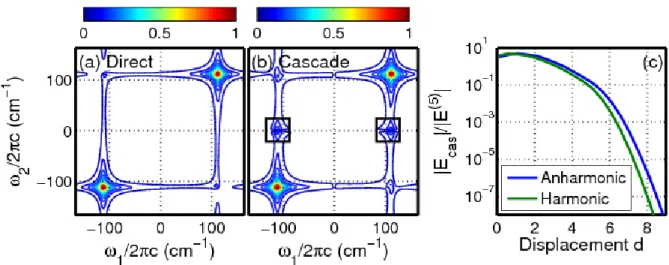
Publishing. ... 5 Figure 1.3. Absolute values of the (a) direct fifth-order and (b) cascaded
third-order signals of triiodide at1=2=112 cm-1 are computed with an empirical anharmonic excited state potential energy surface. The ratio,
(
)
( )5(
)
1, 2 / 1, 2
cas
E E , is computed using (blue) an empirical anharmonic model and (green) a harmonic model with equal ground and excited state frequencies (112 cm-1. 46 The features at
2
=0 cm-1 (enclosed in boxes) in the cascaded signal spectrum represent imperfect subtraction of the non-oscillatory component of the signal, not vibrational resonances. Reproduced from B. M. Molesky, P. G. Giokas, Z. Guo, and A. M. Moran J. Chem. Phys. 141, 114202
(2014), with the permission of AIP Publishing. ... 6 Figure 1.4. State b is first photoexcited then transfers population to state c by
way of an electron transfer transition in the process of interest. Linear reponse rate theories describe the scenario on the left, where thermalization of the wavepacket occurs before electron transfer to state c. The understanding of ultrafast electron transfer processes is complicated by the time-coincident electron transfer and
Figure 1.5. The photoinduced back-electron transfer dynamics of [Ti(cat)3]2- can be described with four potential pathways. The pathway connected by red arrows can be described with traditional models if a Boltzmann distribution of vibrational quanta is established before back-electron transfer; however, a non-equilibrium electron transfer model is required if this condition is not satisfied. The pathways involving vibrational coherences contribute if back-electron transfer is faster than
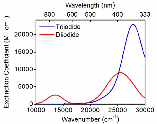
vibrational dephasing. ... 14 Figure 2.1. Linear absorbance spectra of triiodide and diiodide in ethanol. The
absorbance spectrum of triiodide is directly measured, whereas that of diiodide is derived from Reference 35 because it is not stable in solution. Diiodide is probed on the picosecond time scale in the present work. The electronic resonance frequencies associated with this nonequilibrium state of diiodide are likely
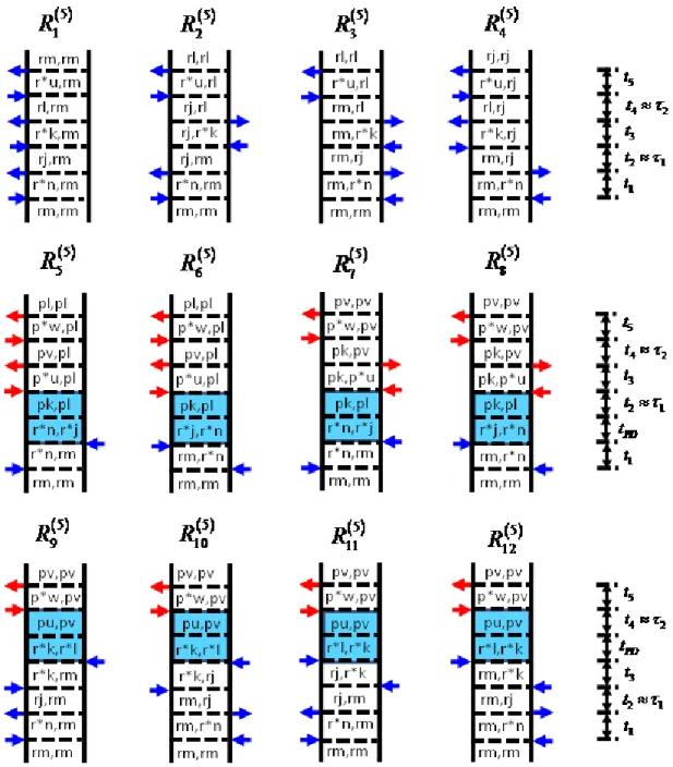
red-shifted from those displayed above... 27 Figure 2.2. Feynman diagrams associated with dominant 2DRR nonlinearities.
Blue and red arrows represent pulses resonant with triiodide and diiodide, respectively. The indices r and r* represent the ground and excited electronic states of the triiodide reactant, whereas p and p* correspond to the diiodide photoproduct. Vibrational levels associated with these electronic states are specified by dummy indices (m,n, j,k,l,u,v,w). Each row represents a different class of terms: (i) both dimensions correspond to triiodide in terms 1-4; (ii) both dimensions correspond to diiodide in terms 5-8; (iii) vibrational
resonances of triiodide and diiodide appear in separate dimensions in terms 9-12. The intervals shaded in blue represent a non-radiative transfer of vibronic
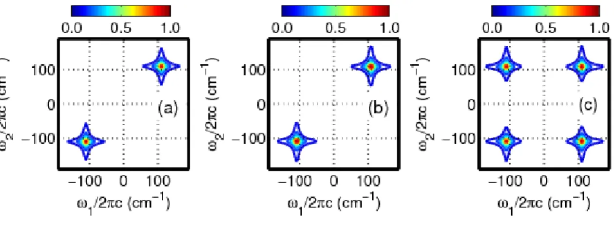
coherence from triiodide to diiodide. ... 32 Figure 2.3. Absolute values of 2DRR spectra computed using (a) the sum of terms
1-4 in Equation (2.22), (b) the sum of terms 5-8 in Equation (2.23), and (c) the sum of terms 9-12 in Equation (2.24). The frequency dimensions, 1 and 2, are conjugate to the delay times, 1 and 2 (see Figure 2.2). Signal components of the type shown in panel (a) are generally detected in one-color experiments. Two-color 2DRR approaches are used to detect nonlinearities that correspond to panels (b) and (c) in this work. The peaks displayed in Figure 2.3c are unique in that
resonances of the reactant and product are found in 1 and 2, respectively. ... 37 Figure 2.4. (a) Diffractive optic-based interferometer used to detect signal
components described by terms 5-8 in Figure 2.2. Each of the two 680-nm beams is split into -1 and +1 diffraction orders with equal intensities at the diffractive optic. The signal is collinear with the reference field (pulse 5) used for
interferometric signal detection. (b) The 340-nm pulse induces photodissociation and vibrational coherence in the diiodide photoproduct during the delay, 1. The time-coincident 680-nm pulses, 2 and 3, reinitiate the vibrational coherence in
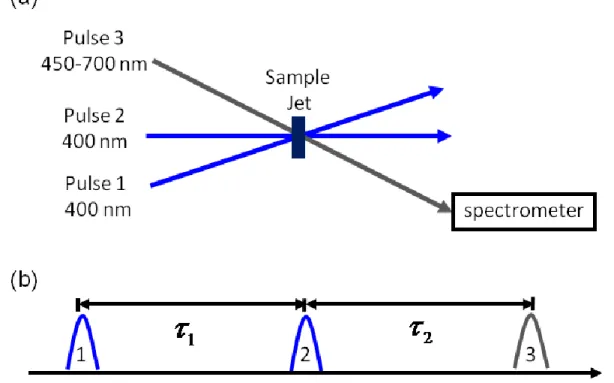
Figure 2.5. (a) Pump-repump-probe beam geometry used to detect signal components described by terms 9-12 in Figure 2.2. (b) The first 400-nm pulse promotes a stimulated Raman response in the ground electronic state of the triiodide reactant during the delay, 1. The second pulse induces
photodissociation of the non-equilibrium reactant, thereby giving rise to vibrational coherence in the diiodide photoproduct during the delay, 2. Sensitivity to diiodide is enhanced by signal detection in the visible spectral
range. ... 42 Figure 2.6. (a) Transient absorption signals (in mOD) obtained for triiodide with a
400-nm pump pulse and continuum probe pulse. (b) The coherent component of the signal is isolated by subtracting sums of 2 exponentials from the total signal presented in panel (a). (c) Fourier transformation of the signal between delay times of 0.1 and 2.5 ps shows that the vibrational frequency decreases as the detection wavenumber decreases. Dispersion in the vibrational frequency reflects sensitivity to high-energy quantum states in the anharmonic potential of
diiodide.19 ... 44 Figure 2.7. 2DRR signals associated with terms 5-8 are obtained using the
two-color approach described in Figure 2.4. (a) The total signal possesses both
coherent and incoherent components. (b) The coherent (Raman) component of the signal is isolated by subtracting sums of two exponentials from the total signal presented in panel (a). (c) The two-dimensional Fourier transformation of the signal in panel (b) in delay ranges, 1 and 2, between 0.15 and 2.0 ps reveals resonances in the upper right and lower left quadrants. This pattern of 2DRR resonances is consistent with calculations based on terms 5-8 (see Figure 2.3),
which this experiment is designed to detect. ... 46 Figure 2.8. 2DRR data are obtained using the two-color approach described in
Figure 2.5. Each column corresponds to a different detection wavenumber: 22,500 cm-1 (444 nm) in column 1; 21,000 cm-1 (476 nm) in column 2; 19,500 cm-1 (513 nm) in column 3; 18,000 cm-1 (555 nm) in column 4. (a)-(d) Total pump-repump-probe signal in mOD. (e)-(h) Coherent parts of the pump-repump-pump-repump-probe signals displayed in the first row. (i)-(l) 2DRR spectra are generated by Fourier
transforming the signals shown in the second row in delay ranges, 1 and 2, between 0.15 and 2.0 ps. The data show that peaks in the upper left and lower right quadrants emerge as the detection wavenumber becomes off-resonant with triiodide. Signals acquired at detection wavenumbers above 21,000 cm-1 (476 nm) are dominated by stimulated Raman processes in the ground electronic state of triiodide (terms 1-4). In contrast, signals acquired at detection wavenumbers below 19,500 cm-1 (513 nm) are consistent with terms 9-12, where vibrational
Figure 2.9. Summary of 2DRR experiments conducted on triiodide: (a) the response of triiodide was detected in both dimensions in Reference 26; (b) the response of the diiodide photoproduct is detected in both dimensions (see Figure 2.7); (c) the response of triiodide and diiodide are detected in separate dimensions (see Figure2.8). Blue and red laser pulses represent wavelengths that are
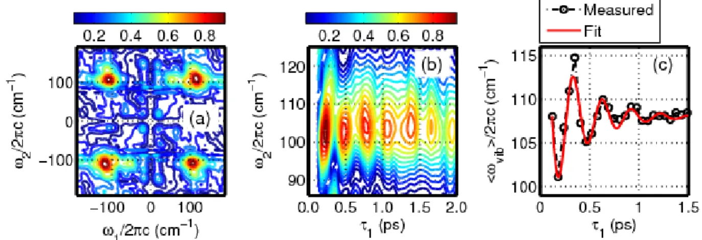
electronically resonant with triiodide and diiodide, respectively. ... 51 Figure 2.10. 2DRR response of triiodide in ethanol with a detection wavenumber
of 19,500 cm-1 (513 nm). (a) Resonances in all four quadrants of the 2DRR spectrum signify cross peaks between triiodide (in 1) and diiodide (in 2). (b) Quantum beats in the Raman spectrum of diiodide are observed when the 2DRR spectrum in panel (a) is inverse Fourier transformed with respect to 1. (c) Oscillations in the mean vibrational frequency are analyzed using Equation (2.6). Such oscillatory behavior suggests that the vibrational coherence frequency of
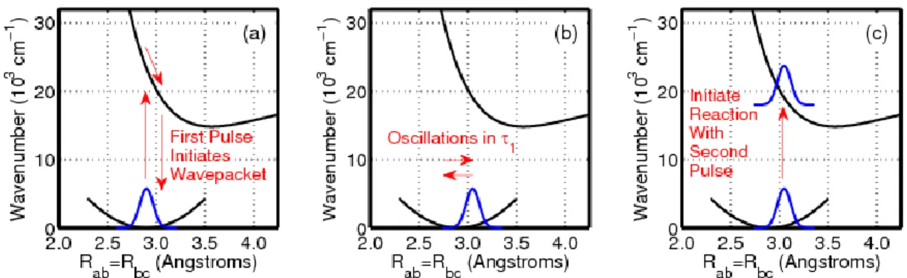
diiodide is sensitive to vibrational motions of triiodide in the delay time, 1. ... 52 Figure 2.11. The sequence of events associated with the 2DRR signals shown in
Figure 2.10. Rab and Rbc denote the two bond lengths in triiodide. (a) The first pulse initiates a ground state wavepacket in the symmetric stretching coordinate. Force is accumulated when both bond lengths increase during the electronic coherence induced by the first laser pulse. (b) Wavepacket motion on the ground state potential energy surface is detected in the delay between the pump and repump laser pulses, 1. (c) Photodissociation of triioide is initiated from a nonequilibrium geometry by the repump laser pulse. The Raman spectrum of
diiodide may then be detected by scanning the delay of a probe pulse, 2. ... 54 Figure 2.12. Correlation between the vibrational wavenumber of the diiodide
photoproduct and the pair of bond lengths in the triiodide reactant, Rab=Rbc, is illustrated by analyzing the dynamics in the mean vibrational coherence frequency, vib
( )
1 , shown in Figure 2.10c. The delay time, 1, is converted into the position of the wavepacket in the symmetric stretching coordinate using the model presented in Figure 2.11. Each revolution of the spiral corresponds to 300 fs. The wavepacket oscillates around the equilibrium bond length until vibrational dephasing is complete. The diagonal slant in the spiral suggests that a bond length displacement of 0.1 Å in triiodide induces a shift of 6.8 cm-1 in thevibrational coherence frequency of diiodide. ... 56 Figure 3.1. The 2DRR technique can be used to detect correlations between
Figure 3.2. Linear absorbance spectra of triiodide and diiodide in ethanol. The absorbance spectrum of triiodide is directly measured, whereas that of diiodide is derived from Reference 44 because it is not stable in solution. The electronic resonance frequencies associated with this nonequilibrium state of diiodide are likely red-shifted from those displayed above. Displacement of the absorbance spectra of triiodide and diiodide facilitates detection of the pathway defined in Figure 3.1. Reproduced from Z. Guo, B. M. Molesky, T. P. Cheshire, A. M. Moran, J. Chem. Phys. 143, 124202 (2015), with the permission of AIP
Publishing. ... 72 Figure 3.3. Feynman diagrams associated with dominant 2DRR nonlinearities.
Blue and red arrows represent pulses resonant with triiodide and diiodide, respectively (see Figure 3.2). The indices r and r* represent the ground and excited electronic states of the triiodide reactant, whereas p and p* correspond to the diiodide photoproduct. Vibrational levels associated with these electronic states are specified by dummy indices (m,n, j,k,l,u,v,w). Each row
represents a different class of terms: (i) both dimensions correspond to triiodide in terms 1-4; (ii) both dimensions correspond to diiodide in terms 5-8; (iii)
vibrational resonances of triiodide and diiodide appear in separate dimensions in terms 9-12. The intervals shaded in blue represent a non-radiative transfer of vibronic coherence from triiodide to diiodide. Reproduced from Z. Guo, B. M. Molesky, T. P. Cheshire, A. M. Moran, J. Chem. Phys. 143, 124202 (2015), with
the permission of AIP Publishing. ... 74 Figure 3.4. Energy level representations associated with individual pathways in
(a) term 1, (b) term 5, and (c) term 9. It is assumed that the chemical reaction is fast compared to the vibrational periods of the reactants and products. Solid and dashed arrows correspond to field-matter interactions with the ket and bra in the
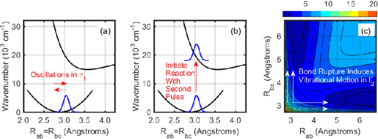
Feynman diagrams presented in Figure 3.3. ... 78 Figure 3.5. The sequence of events associated with terms 9-12 and the pathway in
Figure 3.1. Rab and Rbc denote the two bond lengths in triiodide and must be equal because wavepacket motion in 1 occurs in the symmetric stretching coordinate. (a) The first pulse initiates a ground state wavepacket in the symmetric stretching coordinate. Wavepacket motion on the ground state potential energy surface is detected in the delay between the pump and repump laser pulses, 1. (b)
Photodissociation of triioide is initiated from a nonequilibrium geometry by the repump laser pulse, which separates the 1 and 2 delay times. The Raman spectrum of diiodide may then be detected by scanning the delay of the probe pulse, 2. (c) The repump pulse promotes the wavepacket in triiodide to a steep portion of the excited state potential energy surface. Diiodide is produced by asymmetric motion on the excited state potential energy surface. Adapted from Z. Guo, B. M. Molesky, T. P. Cheshire, A. M. Moran, J. Chem. Phys. 143, 124202
Figure 3.6. Cascades of four-wave mixing signals generally dominate in off-resonant 2D Raman experiments. In the desired ‘direct’ process, all 6 field-matter interactions take place with an individual molecule. The cascaded response is generally negligible in 2DRR spectroscopy because it involves 8 field-matter interactions, whereas the direct process only requires 6. Both types of
nonlinearities are subject to the same selection rules under electronically resonant
conditions. ... 81 Figure 3.7. Absolute values of the (a) direct fifth-order and (b) cascaded
third-order signal magnitudes of triiodide at1=2=112 cm-1 are computed with an empirical anharmonic excited state potential energy surface (see section VIA). The ratio, Ecas
(
1, 2)
/ E( )5(
1, 2)
, is computed using (blue) an empirical anharmonic model and (green) a harmonic model with equal ground and excited state frequencies (112 cm-1) 45. The features at 2=0 cm-1 (enclosed in boxes) in the cascaded signal spectrum represent imperfect subtraction of thenon-oscillatory component of the signal (these are not vibrational resonances). Reproduced from B. M. Molesky, P. G. Giokas, Z. Guo, and A. M. Moran J.
Chem. Phys. 141, 114202 (2014), with the permission of AIP Publishing. ... 82 Figure 3.8. Pulse sequences used to probe terms (a) 1-4, (b) 5-8, and (c) 9-12 in
Figure 3.3. In all cases, the signal is Fourier transformed with respect to the delays, 1 and 2, to generate a 2D spectrum. Blue (deep or near ultraviolet) and red (visible) laser pulses represent resonance with triiodide and diiodide,
respectively. ... 86 Figure 3.9. Diffractive optic-based interferometers used for (a) degenerate
six-wave mixing (with 267-nm beams) and (b) pump (340 nm) degenerate four-six-wave mixing (680 nm). The signal is radiated in the direction ks= k1-k2+k3-k4+k5 in panel (a). The wavevector of the signal is ks=k2-k3+k4 in panel (b) (i.e., the signal wave vector is independent of the direction and color of the 340-nm pump beam). In both cases, the passively phase-stabilized signal field is interferometrically detected using a local oscillator beam (beams 6 and 5 in panels (a) and (b), respectively). (c) Differential transmission of a probe pulse is detected in a pump-repump-probe geometry. The experimental setups in (a) (b), and (c) are used to implement the pulse sequences shown in Figures3.8a, 3.8b, and 3.8c, respectively. Adapted from Z. Guo, B. M. Molesky, T. P. Cheshire, A. M. Moran, J. Chem. Phys. 143, 124202 (2015) and B. M. Molesky, P. G. Giokas, Z. Guo, and A. M. Moran J. Chem. Phys. 141, 114202 (2014), with the permission of AIP
Figure 3.10. Summary of 2DRR experiments conducted on triiodide: (a) the response of triiodide is detected in both dimensions (terms 1-4 in Figure 3.3); (b) the response of the diiodide photoproduct is detected in both dimensions (terms 5-8 in Figure 3.3); (c) the response of triiodide and diiodide are detected in separate dimensions (terms 9-12 in Figure 3.3). Experimental and theoretical 2DRR spectra are presented in the second and third rows, respectively. Calculations in panels (a), (b), and (c) employ Equations (3.22), (3.23), and (3.24). Blue and red laser pulses represent wavelengths that are electronically resonant with triiodide and diiodide, respectively. Adapted from Z. Guo, B. M. Molesky, T. P. Cheshire, A. M. Moran, J. Chem. Phys. 143, 124202 (2015), with the permission of AIP
Publishing. ... 90 Figure 3.11. (a) Fourier transforming the 2DRR signal with respect to only 2
reveals quantum beats of triiodide in the delay time, 1. (b) The average
vibrational frequency of diiodide is computed at each delay point using the signal displayed in panel (a). (c) The delay, 1, is translated into the bond lengths of triiodide. The diagonal slant of the spiral suggests that a bond length displacement of 0.1 Å in triiodide induces a shift of approximately 6.8 cm-1 in the vibrational coherence frequency of diiodide. Adapted from Z. Guo, B. M. Molesky, T. P. Cheshire, A. M. Moran, J. Chem. Phys. 143, 124202 (2015), with the permission
of AIP Publishing. ... 93 Figure 3.12. 2DRR experiments suggest correlation between the geometry of the
wavepacket in triiodide at the time of photodissociation and the distribution of vibrational quanta in the diiodide product. The vibrational coherence frequency of diiodide is smallest when the wavepacket is at the inner turning point of the symmetric stretching mode. This information cannot be obtained from traditional pump-probe experiments where the reaction must be initiated from the
equilibrium geometry of the system. ... 94 Figure 4.1. (a) A four-beam FSRS geometry is used in this work to eliminate the
portion of the background associated with residual Stokes light and a pump-probe response. The color code is as follows: the actinic pump is green, the Raman pump is blue, and the Stokes pulse is red. (b) Vibrational coherences in 1 are resolved by numerically Fourier transforming the signal with respect to the delay time. Time-coincident Raman pump and Stokes pulses then initiate a second set of vibrational coherences, which are resolved by dispersing the signal pulse on an array detector. The fixed time delay, 2, is used to suppress the broadband
pump-repump-probe response of the solution. ... 110 Figure 4.2. Laser spectra are overlaid on the linear absorbance spectra of (a)
Figure 4.3. Diffractive optic-based interferometer used for 2DRR measurements. The transparent fused silica window delays pulse 5 by 290 fs with respect to pulse 4 (delay 2 in Figure 4.1). A four-beam geometry is used to detect the signal radiated in the direction, k1-k2+k3-k4+k5; the wavevectors k1 and k2 cancel each other. The 2DRR signal is obtained by measuring differences with and without the actinic pump (beam 1,2). The indices represent the desired order of field-matter interactions. Beams represented with solid circles reach the sample,
whereas those represented with open circles are blocked with a mask. ... 114 Figure 4.4. 2DRR spectra computed for a pair of harmonic oscillators with
inhomogeneous line broadening. The spectra are computed by combining Equations (4.1) and (4.23) with the parameters given in Table 4.1. The correlation parameter,, is set equal to (a) -0.75, (b) 0.0, and (c) 0.75. The diagonal peaks always exhibit correlated line shapes when the inhomogeneous widths are nonzero, whereas the orientations and intensities of the off-diagonal peaks depend on the correlation parameter, .Table 4.1. Parameters of
Theoretical Model for System with Two Vibrational Modes ... 118 Figure 4.5. 2DRR spectra computed with the anharmonic vibrational Hamiltonian
described in section VB and the parameters in Table 4.1. The diagonal cubic expansion coefficients are set equal to -5 (first row), 0 (second row), and 5 cm-1 (third row). The off-diagonal expansion coefficients are set equal to -5 (first column), 0 (second column), and 5 cm-1 (third column). The response of a harmonic system is shown in panel (e). These calculations suggest that
anharmonic coupling promotes intensity borrowing effects via the transformation of Franck-Condon overlap integrals from the harmonic to anharmonic basis set (see Equation (4.26)). For many of the parameter sets, anharmonicity causes the intensity of the cross peak above the diagonal to increase relative to that of the
cross peak below the diagonal. This effect is most pronounced in the left column. ... 120 Figure 4.6. 2DRR spectrum of myoglobin computed using parameters obtained by
fitting spontaneous resonance Raman excitation profiles.67 The spectrum is dominated by resonances on the diagonal. The most dominant cross peak is associated with the iron-histidine stretch (1/ 2c=220 cm-1) and in-plane stretching mode (2/ 2c=1356 cm-1). The spectra are computed by combining
(A20) with the parameters in Table 4.2. ... 124 Figure 4.7. Signals obtained for (a) metMb and (d) MbO2 in a FSRS-like
representation. At each point in 2, the incoherent baseline is generated using the maximum entropy method. Shown here are slices of the signals for (b) the 670-cm-1 mode of metMb and (e) the 370-cm-1 mode of MbO2. Coherent residuals are obtained by subtracting incoherent MEM baselines from the total signals for (b) metMb and (e) MbO2. The coherent residuals are presented for (c) metMb and (f)
Figure 4.8. Molecular structure of iron protoporphyrin-IX. ... 126 Figure 4.9. Experimental 2DRR spectra for (a) metMb and (b) MbO2 are
generated by Fourier transforming the coherent residuals with respect to 1 at each point in 2 (i.e., at each pixel on the CCD detector). For both systems, diagonal peaks are detected near 220, 370, 674, and 1356 cm-1 (close to 1373 cm-1
in metMb). Arrows are used to identify cross peaks. ... 129 Figure 4.10. Line shapes of diagonal peaks are examined in lower-frequency
regions of 2DRR spectra obtained for (a) metMb and (b) MbO2. Peaks are fit to two-dimensional Gaussians with correlation parameters given in panels (c) and (d) (see Equation (4.2)). The parameter, , ranges between the uncorrelated (=0) and fully correlated (=1) limits for diagonal peaks. A correlation parameter greater than 0 is a signature of inhomogeneous line broadening. In panels (e) and (f), a straight line consistent with each correlation parameter is overlaid on the experimental data. For both systems, the 370-cm-1 methylene deformation mode local to the propionic acid side chains exhibits the greatest
amount of heterogeneity. ... 130 Figure 4.11. Dihedral angles associated with the propionic acid chains are defined
for the heme in (a) metMb and (d) MbO2. The vibrational frequency of the methylene deformation mode local to the propionic acid side chains is computed as a function of the two dihedral angles for (b) metMb and (e) MbO2. These ab initio maps are used to parameterize the vibrational frequencies associated with molecular dynamics simulations. Segments of molecular dynamics trajectories for
the vibrational frequencies are shown for (c) metMb and (f) MbO2. ... 133 Figure 4.12. Spectral densities of the methylene deformation modes obtained from
molecular dynamics simulations. The spectral densities decay to less than 50% of the maximum values at frequencies corresponding to the fluctuation amplitudes (5.9 and 7.0 cm-1 for metMb and MbO2). These calculations are consistent with an
intermediate line broadening regime. ... 135 Figure 5.1. a) Six-wave mixing process for p-nitroaniline. Cascade of four-wave
mixing responses between b) two nitroaniline molecules and c) methanol and
p-nitroaniline. ... 149 Figure 5.2. (a) Pulse sequence used in FSRS-like approach in which only one
delay time, 1, is scanned. A fixed delayfixed is introduced to suppress undesired pump-repump-probe nonlinearities. (b) Pulse sequence used in all-broadband approach in which two experimentally controlled delay times, 1 and 2, are scanned. The 2DRR spectrum is obtained by 2D Fourier transformation of the
signal. ... 152 Figure 5.3. FSRS signals for p-nitroaniline in acetonitrile were computed using
direct FSRS response, and (c) the total FSRS signals are simulated under the
conditions of AP =RP =eg... 157 Figure 5.4. Raman shift for p-nitroaniline in acetonitrile at 861 cm-1 (top) and
1326 cm-1 (bottom). (a) & (d) Cascaded response of the solute, (b) & (e) the direct FSRS signal, and (e) & (f) the logarithm of the ratio of the signal fields
(
( ) ( ))
,
log10 ESolute Solute Cas3 − / EFSRS5 are computed using the parameters in Table 5.1. The horizontal axis represents the detuning of the actinic and Raman pump beams from the electronic resonance frequency. The linear scaling factor for the mode displacements is given on the vertical axis. The unscaled dimensionless mode
displacements are 1.5 for both the 861 cm-1 (top) and 1326 cm-1 mode (bottom). ... 158 Figure 5.5. Spectra for p-nitroaniline in methanol computed using the parameters
in Table 5.1. Cascades from solute-solvent interactions (a), direct fifth-order (b),
and the total FSRS (c) signals are simulated under the condition AP =RP =eg. ... 160 Figure 5.6. Raman shift for p-nitroaniline in methanol at 861 cm-1 (top) and 1328
cm-1 (bottom). (a) & (d) Cascaded response of the solvent, (b) & (e) the direct FSRS signal, and (e) & (f) the logarithm of the ratio of the signal fields
(
( ) ( ))
,
log10 ESolute Solvent Cas3 − / EFSRS5 are computed using the parameters in Table 5.1. The horizontal axis represents the detuning of the actinic and Raman pump beams from the electronic resonance frequency. The linear scaling factor for the mode displacements is given on the vertical axis. The unscaled dimensionless mode
displacements are 1.5 for both the 861 cm-1 (top) and 1326 cm-1 mode (bottom). ... 161 Figure 5.7. The ratio of the electric fields ESolute Solvent Cas( )3 − , / EFSRS( )5 were computed
for the Raman shift of p-nitroaniline at 861 cm-1 (red, top inset) and 1328 cm-1 (blue, bottom inset) using the methanol parameters in Table 5.1 and varying the solvent vibrational mode. The horizontal axis (vertical axis of the inset) represents the solvent mode. The detuning of the actinic and Raman pumps from the
electronic resonance is set to 0 cm-1 in the parent Figure and varies along the horizontal axes for the inset. The vertical axis (colorbar of the inset) gives values
of the electric fields ratio. ... 162 Figure 5.8. Spectra for p-nitroaniline in dichloromethane were computed using the
parameters in Table 5.1. Cascades from solute-solute and solute-solvent
interactions (a), direct fifth-order (b), and the total FSRS (c) signals are simulated
Figure 5.9. Spectra for p-nitroaniline in acetonitrile were computed using the parameters in Table 5.1. Cascades from solute-solute interactions (a), direct fifth-order (b), and the total 2DRR (c) signals are simulated under the condition
L eg
= . ... 164 Figure 5.10. Raman shift for p-nitroaniline in acetonitrile at 861 cm-1 (top) and
1326 cm-1 (bottom). (a) & (d) Cascaded response of the solute, (b) & (e) the direct 2DRR signal, and (e) & (f) the logarithm of the ratio of the signal fields
(
( ) ( ))
,
log10 ESolute Solute Cas3 − / E2 DRR5 are computed using the parameters in Table 5.1. The horizontal axis represents the detuning of the impinging laser pulses from the electronic resonance. The linear scaling factor for the mode displacements is given on the vertical axis. The unscaled dimensionless mode displacements are
0.84 and 0.98 for the 861 cm-1 (top) and 1326 cm-1 mode (bottom). ... 165 Figure 5.11. Spectra for p-nitroaniline in methanol were computed using the
parameters in Table 5.1. (a) Cascades from solute-solvent interactions, (b) direct
fifth-order, and (c) the total 2DRR, all simulated under the condition L =eg... 166 Figure 5.12. Raman shift for p-nitroaniline in methanol at 861 cm-1 (top) and 1326
cm-1 (bottom). (a) & (d) Cascaded response of the solvent, (b) & (e) the direct 2DRR signal, and (e) & (f) the logarithm of the ratio of the signal fields
(
( ) ( ))
,
log10 ESolute Solvent Cas3 − / E2 DRR5 are computed using the parameters in Table 5.1. The horizontal axis represents the detuning of the impinging laser pulse from the electronic resonance. The linear scaling factor for the mode displacements is given on the vertical axis. The unscaled dimensionless mode displacements are
1.5 for both the 861 cm-1 (top) and 1326 cm-1 mode (bottom). ... 167 Figure 5.13. The ratio of the electric fields ESolute Solvent Cas( )3 − , / E2dRR( )5 were computed
for the Raman shift of p-nitroaniline at 861 cm-1 (red, top inset) and 1328 cm-1 (blue, bottom inset) using the methanol parameters in Table 5.1 and varying the solvent vibrational mode. The horizontal axis (vertical axis of the inset) represents the solvent mode. The detuning of the incident laser pulses from the electronic resonance is set to 0 cm-1 in the parent Figure and varies along the horizontal axes for the inset. The vertical axis (colorbar of the inset) gives values of the electric
fields ratio. ... 168 Figure 5.14. Spectra for p-nitroaniline in dichloromethane were computed using
the parameters in Table 5.1. Cascades from solute-solute and solute-solvent interactions (a), direct 2DRR (b), and the total 2DRR (c) signals are simulated
Figure 5.15. Feynman diagrams associated with the direct fifth-order response. The indices, g and e, represent the ground and excited electronic states, whereas dummy indices (m,n,k,l,u, and v) denote vibrational levels. Green, blue, and red arrows represent the actinic pump, Raman pump, and Stokes pulses,
respectively. ... 169 Figure 5.16. Feynman diagrams associated with the direct fifth-order 2DRR
response. The indices, g and e, represent the ground and excited electronic states, respectively, whereas dummy indices (m,n,k,l,u, and v) denote
vibrational levels. ... 172 Figure 5.17. Feynman diagrams associated with (a) pump-probe and (b) CSRS
components to FSRS cascades written in a sum-over-states representation. The indices, g and e, represent the ground and excited electronic states, respectively, whereas dummy indices (m,n,k, and l) denote vibrational levels. Field-matter interactions are color-coded as follows: actinic pump is green; Raman pump is blue; Stokes is red; radiated signal field is red; the field radiated at the
intermediate step in the cascade is black. ... 175 Figure 5.18. Feynman diagrams associated with third-order cascades with the
intermediate phase-matching condition k1-k2+k5. The indices, g and e, represent the ground and excited electronic states, respectively, whereas dummy indices (m,n,k, and l) denote vibrational levels. Field-matter interactions are color-coded as follows: actinic pump is green; Raman pump is blue; Stokes is red; radiated signal field is red; the field radiated at the intermediate step in the
cascade is black. ... 178 Figure 5.19. Feynman diagrams associated with third-order cascades with the
intermediate phase-matching condition k3-k4+k5. The indices, g and e, represent the ground and excited electronic states, respectively, whereas dummy indices (m,n,k, and l) denote vibrational levels. Field-matter interactions are color-coded as follows: actinic pump is green; Raman pump is blue; Stokes is red; radiated signal field is red; the field radiated at the intermediate step in the
cascade is black. ... 179 Figure 5.20. Feynman diagrams associated with 2DRR cascades written in a
sum-over-states representation. The indices g and e refer to the ground and excited
electronic states, respectively. ... 180 Figure 5.21. Summary of sequential cascades with the intermediate phase
matching condition k1-k2+k3 on molecule A. The field radiated by molecule A (blue arrow) induces one of the first two field-matter interactions on molecule B (blue arrow). Feynman diagrams for molecules A and B involve sums over
Figure 5.22. Summary of sequential cascades with the intermediate phase matching condition, -k1+k2+k4. The field radiated by molecule A (blue arrow) induces one of the first two field-matter interactions on molecule B (blue arrow). Changing the signs of the wavevectors for pulses 1, 2, and 4 translates into complex conjugation of the term in the response function associated with molecule A. Feynman diagrams for molecules A and B involve sums over
independent dummy indices for vibrational levels (m, n, k, l). ... 183 Figure 5.23. Parallel cascades with the intermediate phase matching condition
k1-k2+k5 and k3-k4+k5 on molecule A are both summarized here. The field radiated by molecule A (blue arrow) induces the third field-matter interaction on molecule B (blue arrow). Feynman diagrams for molecules A and B involve sums over
independent dummy indices for vibrational levels (m, n, k, l). ... 184 Figure 6.1. The photo-induced back-electron transfer dynamics of [Ti(cat)3]2- can
be described with four potential pathways. The pathway connected by red arrows can be described with traditional models if a Boltzmann distribution of vibrational quanta is established before back-electron transfer; however, a non-equilibrium electron transfer model is required if this condition is not satisfied. The pathways involving vibrational coherences contribute if back-electron transfer is faster than
vibrational dephasing. ... 190 Figure 6.2. Nonlinearities associated with the hot ground state signal component
can be obtained by incorporating two field-matter interactions before and after the back-electron transfer process. The time intervals, ti, separate perturbative
interactions with an external electric field, ˆHrad mat− (blue arrows), and the donor-acceptor coupling, ˆV (red arrows). The indices g and e represent ground and excited states of [Ti(cat)3]2-, whereas the vibrational levels are represented by dummy indices (m, n, k, l, u, v). The indices m , l, and u are associated with the ground electronic state, whereas n, k, and v correspond to the excited electronic state. The non-radiative transition from state e to state g is referred to as
“back-electron transfer” (i.e., the events shaded in blue). ... 195 Figure 6.3. The measured absorption spectrum is fit with Equation (6.19) and the
parameters in Table 6.1. The absorption cross section, A, is used to fit the low-energy side of the line shape subject to the constraints imposed by the Raman cross sections. An additional Gaussian line shape (green) is used to estimate the
contribution of the second-to-lowest energy transition to the total absorbance. ... 207 Figure 6.4. Resonance Raman spectrum of [Ti(cat)3]2- acquired in aqueous
solution with excitation at 488 nm. ... 208 Figure 6.5. Experimental Raman cross sections are fit using Equation (6.20) and
Figure 6.6. The (a) experimental transient absorption signal acquired under the magic angle polarization condition is (b) fit using Equation (6.23). The residual shows that agreement between the experiment in fit is best at delay times greater
than 60 fs (i.e., outside the region of pulse overlap). ... 212 Figure 6.7. (a) The magnitude of the HGS signal component rises until a delay
time of 0.5 ps before vibrational cooling causes the signal to decay. The GSB signal component rises instantaneously and decays on the time scale of vibrational cooling. (b) The HGS signal component shifts to shorter wavelengths because of vibrational cooling, whereas the peak of the GSB resonance is insensitive to the delay time. (c) The FWHM of the HGS resonance decreases by 50% within the first 3 ps, whereas the line width of the GSB is insensitive to the delay time. The 100 fs time scale of the BET process is the key information provided by these
data. ... 214 Figure 6.8. The coherent component of the transient absorption response of
[Ti(Cat)3]2- is analyzed for a range of detection wavelengths. Coherent vibrational motion is detected at wavelengths that correspond to the HGS signal component. The stimulated Raman response for the GSB signal component is comparable to the noise level of the experiment. This measurement demonstrates that the BET process initiates vibrational motions, which represent pathways that end in the
upper right of Figure 6.1. ... 217 Figure 6.9. (a) An incoherent baseline is subtracted from the isotropic signal
component at 500 nm to (b) isolate the coherent response. (c) Fourier
transformation yields a coherent Raman spectrum for the isotropic HGS signal component. (d) An incoherent baseline is subtracted from the anisotropic signal component at 500 nm to (e) isolate the coherent response. (f) Fourier
transformation yields a coherent Raman spectrum for the anisotropic HGS signal component. All mode frequencies are slightly smaller than those observed with spontaneous Raman spectroscopy, which indicates that the modes are highly populated following back-electron transfer (i.e., the frequencies are lower because
of anharmonicity). ... 219 Figure 6.10. Physical picture suggested by theoretical model. (a) The pump pulse
initiates a wavepacket in the collective ‘solvent’ coordinate, which moves toward the point of intersection between potential energy surfaces as increases. Energy is (linearly) mapped onto the collective coordinate for convenience. (b) Motion of the wavepacket, Y
( )
,q , is simulated with Equation (6.24). (c) Growth in the magnitude of the doorway function with represents an increase in theprobability of a BET transition. Quantized vibrational modes must promote the BET transition deep within the inverted regime, because the excited state
wavepacket possesses little overlap with the geometry of the transition state in the
Figure 6.11. Doorway functions, Di→j
( )
, are computed with Equation (6.14) and the parameters in Table 6.1. Only the 222 cm-1 mode is included in these calculations. The times, , are (a) 0.2, (b) 0.5, and (c) 2 ps. The calculations suggest that vibrational coherences are initiated in the ground electronic state following BET if the system is initially in either a vibrational coherence (upper right) or population (lower right). The behavior transitions from an energygap-limited regime at =0.1 ps to a Franck-Condon-limited regime at =2 ps. ... 224 Figure 6.12. Doorway functions, Di→j
( )
, are computed with Equation (6.14)and the parameters in Tables 6.1 and 6.2 (the mode displacement is taken from Table 6.2). Only the 1482 cm-1 mode is included in these calculations. The times,
, are (a) 0.2 ps, (b) 0.5 ps, (c) 2 ps. The calculations suggest that vibrational coherences are initiated in the ground electronic state following BET if the system is initially in either a vibrational coherence (upper right) or population (lower right). These calculations show that all pathways will generally be activated in systems with high-frequency (>1000 cm-1) vibrational modes and charge transfer
resonances in the visible spectral range. ... 225 Figure 6.13. (a) Fourier transform of transient absorption signal calculated with
Equation (6.27) and the parameters in Tables 6.1 and 6.2. This contour plot can be compared to the measurement in Figure 6.8. The calculated and measured signals are overlaid at a detection wavelength of (b) 500 nm and (c) 550 nm. The
parameters are adjusted to optimize the fit to the absorbance spectrum (Figure 6.3), the resonance Raman cross sections (Figure 6.5), and the fit to the transient
absorption signal at 500 nm (Figure 6.13b). ... 227 Figure 6.14. We consider whether or not population-to-coherence pathways are
relevant in systems regardless of the electron transfer time-scale. (a) Only population-to-population transitions occur in the traditional second order rate formula, Equation (6.29). The population-to-coherence pathway survives if the trace is taken only over electronic states in Equation (6.30). (b) In a higher-order model, a trace over all quantum states can be carried out if subsequent vibrational cooling dynamics are accounted for. Vibrational population-to-coherence
transitions may then contribute regardless of the electron transfer rate. The operators ˆV and ˆV denote the donor-acceptor coupling and the solute-solvent
interaction, respectively. ... 231 Figure 6.15. The electronic structure can be viewed in (a) localized and (b)
delocalized basis sets. (c) The transient absorption anisotropy associated with the HGS signal component agrees well with the prediction of 0.1, which is
independent of the basis set. The uncertainty in the anisotropy is approximately 0.05. The anisotropy in the HGS signal component should not be used to argue for
Figure A.1. Fenyman diagrams associated with dominant 2DRR nonlinearities. Blue and red arrows represent pulses resonant with triiodide and diiodide, respectively. The indices r and r* represent the ground and excited electronic states of the triiodide reactant, whereas p and p* correspond to the diiodide photoproduct. Vibrational levels associated with these electronic states are specified by dummy indices (m,n, j,k,l,u,v,w). Each row represents a different class of terms: (i) both dimensions correspond to triiodide in terms 1-4; (ii) both dimensions correspond to diiodide in terms 5-8; (iii) vibrational
resonances of triiodide and diiodide appear in separate dimensions in terms 9-12. The intervals shaded in blue represent a non-radiative transfer of vibronic
coherence from triiodide to diiodide. ... 252 Figure A.2. Comparison of signal phases obtained for third-order (pump-probe)
and fifth-order (pump-repump-probe) signals. (a) Pump-probe (delay of 0.5 ps) and pump-repump-probe (1=2=0.5 ps) signals have similar line shapes but opposite signs. This sign-difference suggests that the pump-repump-probe signal is dominated by the desired fifth-order nonlinearity (i.e., not third-order cascades). (b) Oscillations in pump-probe and pump-repump-probe signals are compared with signal detection at 20,000 cm-1 (500 nm). This is a slice of the
pump-repump-probe signal in 2 with the delay, 1, fixed at 0 ps. A relative phase-shift near 180º suggests that the oscillatory component of the pump-repump-probe
signal is dominated by the direct fifth order nonlinearity.8 ... 261 Figure A.3. Spectral components associated with oscillations of the mean
vibrational resonance frequencies computed with an anharmonic vibrational Hamiltonian. The diagonal expansion coefficients are set equal to -5 (first row), 0 (second row), and 5 cm-1 (third row). The off-diagonal expansion coefficients are set equal to -5 (first row), 0 (second row), and 5 cm-1 (third row). All amplitudes are normalized to the maximum found for the 400-cm-1 mode in the second row and first column. These calculations show that oscillations in the mean vibrational resonance frequencies occur primarily at the difference frequency in the harmonic system (see panel (e)). Anharmonicity increases the amplitude of oscillations at
the fundamental frequencies of the vibrations. ... 265 Figure A.4. Distribution of dihedral angles for 5000 steps of the molecular
dynamics trajectory simulated for metMb. The equilibrium dihedral angles
associated with the propionic acid side chains (see Figure 3.11) are L=81.3° and R
=81.1°. ... 266 Figure A.5. Distribution of dihedral angles for 5000 steps of the molecular
dynamics trajectory simulated for MbO2. The equilibrium dihedral angles
associated with the propionic acid side chains (see Figure 3.11) are L=94.4° and R
Figure A.6. Parameters of a broadband signal component determined in the decomposition of transient absorption signals. (a) Magnitude of the broadband signal component. (b) Peak wavelength computed for the broadband signal component. (c) FWHM line width for the broadband signal component. It is necessary to include a signal component at longer wavelengths because discontinuities in the parameters of the GSB and HGS resonances are found
otherwise. ... 270 Figure A.7. The measured absorption spectrum is fit with Equation (4.19) in the
main article and the parameters in Table A.1. The absorption cross section, A, is used to fit the low-energy side of the line shape subject to the constraints imposed by the Raman cross sections. A Gaussian line shape (green) is used to estimate the
contribution of the second-to-lowest energy transition to the total absorbance. ... 271 Figure A.8. Experimental Raman cross sections are fit using Equation (4.20) in
the main article and the parameters in Table A.1. ... 272 Figure A.9. The measured absorption spectrum is fit with Equation (4.19) in the
main article and the parameters in Table S2. The absorption cross section, A, is used to fit the low-energy side of the line shape subject to the constraints imposed by the Raman cross sections. A Gaussian line shape (green) is used to estimate the
contribution of the second-to-lowest energy transition to the total absorbance. ... 275 Figure A.10. Experimental Raman cross sections are fit using Equation (4.20) and
the parameters in Table A.2. ... 276 Figure A.11. The coherent response of the [Ti(cat)3]2- is analyzed for a range of
detection wavelengths. Coherent vibrational motion is detected at wavelengths that correspond to the HGS signal component in the 450-560-nm range. The stimulated Raman response for the GSB signal component is relatively weak. These data suggest that the back electron transfer process induces the vibrational
motions detection in our transient absorption experiments. ... 278 Figure A.12. Linear absorbance spectra of [Ti(cat)3]2- and catechol on a TiO2
nanocrystalline film. Both measurements are conducted in aqueous solution. ... 281 Figure A.13. (a) Transient absorption contour plot for the chirp-corrected signal
from catechol on TiO2 . Scatter of the pump pulse at 410 nm has been removed to preserve the color scale. The spectrum shows a 25-mOD GSB repsonse at 440 nm, a blue-shifting HGS resonance near 550 nm, and an absorptive feature at longer wavelengths. (b) Gaussian functions are used to fit the experimental
Figure A.14. Decomposition of GSB, HGS, and broadband signal components for catechol on TiO2. (a) The peak wavelength of the GSB portion of the spectrum is insensitive to the delay time. (b) The HGS signal component blue-shifts and narrows as the delay increases. c) The long-lived feature centered above 700 nm
LIST OF ABBREVIATIONS 2DRR Two-dimensional resonance Raman
AP Actinic pump
BBO Beta barium borate BET Back electron transfer CCD Charge-coupled device
CMOS Complementary metal oxide semiconductor CSRS Coherent stimulated Raman spectroscopy
CT Charge transfer
DOS Density of States
EFRC Energy Frontier Research Center ESA Excited state absorption
ESE Excited state emission ET Electron transfer
FSRS Femtosecond stimulated Raman spectroscopy FWHM Full width half maximum
GSB Ground state bleach HGS Hot ground state
HWHM Half width half maximum LEPS London-Eyring-Polanyi-Sato LMCT Ligand to metal charge transfer
MD Molecular dynamics
MEM Maximum entropy method PP Pump-probe spectroscopy
RP-D4WM Resonant pump degenerate four wave mixing
St Stokes pulse
TR-ISRS Time resolved impulsive stimulated Raman spectroscopy TRSRS Time resolve spontaneous Raman spectroscopy
UV Ultraviolet
LIST OF SYMBOLS
1D One dimensional
2D Two dimensional
( )
A Molecular absorption spectrum a Annihilation operator
†
a Creation operator 2
Polarizability magnitude squared
( )
Frequency dependent polarizability
( )
t Time dependent polarizability
Å Angstrom
atm Atmosphere m
B Boltzmann population of a vibrational state, such that m is an integer representing the vibrational state
C Concentration
c Speed of light 2
CaF Calcium fluoride cm Centimeter
1
−
cm Wavenumber 2
CS Carbon disulfide ( )
n
Susceptibility of nth order
D Debye
( )
D Time dependent vibrational wavepacket
( )
2
Variance in electronic energy gap d Dimensionless displacement
( )
E t Electric Field ( )n
E Signal field of nth order i
E Energy level of statei, where i can be an electronic or vibrational energy e Electronic excited state index
eV Electron volt 0
Vacuum permittivity
fs Femtosecond
( )
L R Dihedral angle
(
a, b)
G Two dimensional Gaussian distribution 0
Geg Free energy gap
g Electronic ground state index
/
g mm Grooves per millimeter
/
g mol Molar mass
eg Electronic dephasing
ij Dephasing of states i and j , where i and jare vibrational states rp Reactant-product dephasing
vib Vibrational dephasing
( )
t Line broadening function H Hamiltonian operator
a Deviation of harmonic mode frequency, a.
2
−
I Diiodide
3
−
I Triiodide
( )
J Vibrational wavepacket ( )n
K Rate function of nth order k Rate constant
i
k Wavevector i, where i represents field-matter interaction
B
k Boltzmann constant kHz Kilohertz
KI Potassium iodide
l Path length
AP Actinic pump pulse width RP Raman pump pulse width UV UV pump pulse width VIS VIS pump pulse width
1
−
Time scale of nuclear relaxation
Reorganization energy
( )
t Absorption peak wavelength
( )
L Line shape function
m mass
J Microjoule m Micrometer mL Milliliter mm Millimeter mM Milli molar mmol Milli mole
mOD Milli optical density
ˆ
Dipole operator
ij Transition dipole magnitude between statesiand j, whereiand jare electronic states
N Number of ‘particles’ A
N Avogadro’s number
m
N Number of vibrational quanta of normal mode in basis m
nJ Nanojoule
nm Nanometer
ns Nanosecond
( )
n Frequency dependent refractive index
Angular frequency
h eg Electronic energy gap
h ij Energy difference between statesiand j, where iand jcan be electronic, vibrational, or vibronic states
h vib Vibrational energy difference
a Average harmonic mode frequency, a
L Carrier frequency of incident light
RP Raman pump frequency
UV UV pump frequency
VIS VIS pump frequency
( )
vib Average vibrational frequency ( )n
P Nth order polarization
( )
*p p Ground (excite) state index of product ps Picosecond
Q Primary oscillator coordinate q Generalized coordinate
( )n
R Nth order response function
( )
*r r Ground (excite) state index of reactant Inter-mode correlation parameter
,
i j Density matrix element for statesiand j, where iand jare vibronic states ( )
(
)
,
n
S Signal of n field-matter interactions
P
S Signal of parallel pump and probe
⊥
S Signal of perpendicular pump and probe
A Absorption cross-section
a Width of inhomogeneous distribution in mode, a
R Raman differential cross-section
t Time variable
Time delay/interval
Ti Titanium
( )
23
−
Ti cat Titanium catechol anion
2
TiO Titanium dioxide
ijk
U Cubic expansion coefficient
eg
V Donor-acceptor coupling
AP Actinic pump electric field amplitude
L Carrier pulse electric field amplitude
RP Raman pump electric field amplitude
St Stokes pulse electric field amplitude
UV UV pump electric field amplitude
CHAPTER I: INTRODUCTION I. Overview
The central theme of this dissertation is the evolution of ideas from the feedback between experiment and theory. In this chapter, the history of multidimensional Raman spectroscopy and its challenges are explored as a foundation to the research in later chapters. The progress made in the field of multidimensional Raman spectroscopy would not have been possible without the parallel development in the theory of nonlinear optical spectroscopy. Chapters 2 and 3 will discuss the development of two-dimensional resonant Raman (2DRR) spectroscopy in the context of coherence transfer during the photodissociation reaction of triiodide. Coherence transfer is further discussed in chapter 6, as it relates to back-electron transfer in a transition metal complex. Chapter 4 investigates heterogeneity in the spectra of oxygen- and water-ligated myoglobin. And in chapter 7, the persistent challenge of cascading signals is explored in detail. Through these topics, this dissertation aims to accomplish the following:
• Development of six-wave mixing response functions for higher-order Raman spectroscopies
• Development of a model that yields transient absorption signatures of vibronic coherence transfer processes coupled to a chemical reaction
• Use simulations of 2DRR line shapes of myoglobin with molecular dynamics simulations and an ab initio map to analyze line broadening mechanisms
II. Promises and Pitfalls of Multidimensional Raman Spectroscopies IIA. History of Higher-Order Raman Spectroscopies
Once the specialty of a handful of experimental groups, multidimensional laser
spectroscopies have become fairly widespread in the past 20 years with applications spanning the traditional disciplines of chemistry, biology, and physics. A technique commonly referred to as two-dimensional spectroscopy, which adds a “pump” dimension to traditional pump-probe spectroscopy, is the most commonly employed multidimensional technique, but this was not always the case.1-10 The development of modern multidimensional laser spectroscopies is rooted in the coherent Raman spectroscopies of the late 1970’s and early 1980’s.11-14 It was unclear at the time whether or not traditional one-dimensional coherent Raman measurements could distinguish homogeneous and inhomogeneous line broadening mechanisms. Landmark
theoretical papers by Mukamel and co-workers showed that higher-order (i.e. multidimensional) methods were indeed required,15-16 and early success was achieved in Raman echo experiments (i.e., eight-wave mixing).17 Several experimental groups took up the challenge of six-wave mixing experiments in the mid-1990’s but met substantial technical challenges.18-22 Success in these six-wave mixing measurements was achieved after nearly a decade of exhaustive efforts. 22-23 Problems encountered in these pioneering works significantly slowed the development of multidimensional Raman techniques. However, interest in this class of experiments has been reinitiated by related methods used to study molecular photochemistries.24-28 The techniques developed in this dissertation involve aspects of both the old and new versions of
multidimensional Raman spectroscopies.
spontaneous Raman transition). Nonetheless, TRSRRS are among the most indispensible tools used to investigate photochemistries because resonance enhancement enables studies of dilute solutions and active sites in complex systems.29-33 In TRSRRS, the process of interest is initiated with a laser pulse before interrogation with a time-delayed resonance Raman probe. Structural changes that accompany a wide variety of chemical reactions can be elucidated in this way (e.g., photochemical ring opening, proton transfer, and isomerization).34-36 Despite strong selling points for studies of slower processes, TRSRRS experiments are inherently insensitive to
dynamics on the 100-fs time-scale because of the tradeoff between time and frequency resolution made in the probing step. In essence, the spontaneous nature of the probe translates into
uncertainty in the delay between the excitation and detection processes.
Figure 1.1. Key ideas associated with FSRS and TR-ISRS are illustrated with energy level