Electrostatics of solvated systems in periodic boundary conditions
Oliviero Andreussi1,2,*and Nicola Marzari1,†
1Theory and Simulations of Materials (THEOS), and National Center for Computational Design and Discovery of Novel Materials
(MARVEL), ´Ecole Polytechnique F´ed´erale de Lausanne, Station 12, 1015 Lausanne, Switzerland 2Department of Chemistry, University of Pisa, Via Moruzzi 3, 56124 Pisa, Italy
(Received 27 June 2014; revised manuscript received 28 October 2014; published 1 December 2014) Continuum solvation methods can provide an accurate and inexpensive embedding of quantum simulations in liquid or complex dielectric environments. Notwithstanding a long history and manifold applications to isolated systems in open boundary conditions, their extension to materials simulations, typically entailing periodic boundary conditions, is very recent, and special care is needed to address correctly the electrostatic terms. We discuss here how periodic boundary corrections developed for systems in vacuum should be modified to take into account solvent effects, using as a general framework the self-consistent continuum solvation model developed within plane-wave density-functional theory [O. Andreussiet al.,J. Chem. Phys.136,064102(2012)]. A comprehensive discussion of real- and reciprocal-space corrective approaches is presented, together with an assessment of their ability to remove electrostatic interactions between periodic replicas. Numerical results for zero- and two-dimensional charged systems highlight the effectiveness of the different suggestions, and underline the importance of a proper treatment of electrostatic interactions in first-principles studies of charged systems in solution.
DOI:10.1103/PhysRevB.90.245101 PACS number(s): 31.15.−p,31.70.Dk,71.15.Dx,71.15.Mb
I. INTRODUCTION
Computer simulations of materials have been significantly progressing in recent years due to the many improvements in both computational tools and underlying algorithms. In particular, density-functional theory (DFT) has become a very valuable tool to model complex systems with high accuracy. Even though a large effort in the field has been devoted to advancing the accuracy of the algorithms beyond the level of DFT, these improvements usually come with a substantial increase of the computational costs, therefore imposing some serious limitations on the system sizes that can be handled. For this reason, hierarchical algorithms have been developed, which allow us to treat different parts of the systems with different degrees of accuracy, without compromising the description of the important atomistic features that need to be characterized.
Among hierarchical methods, a fundamental role has been played by continuum dielectric models, which combined with
ab initioand DFT atomistic calculations have been shown to be very effective in modeling solvents and complex environments in an inexpensive and accurate way [1–4]. Although most of the continuum dielectric models have been developed in the chemistry community and applied to study isolated systems, a large effort has been spent in recent years to extend these models to the boundary between condensed matter physics and chemistry [5–12]. In particular, the possibility of reducing the computational complexity of solvated or electrified interfaces would allow the extensive modeling of a large range of fundamental processes, such as those taking place in heterogeneous catalysis, electrochemistry, and photochemistry.
*[email protected] †[email protected]
We recently proposed a self-consistent continuum solvation (SCCS) model [5,7,13] that combines a highly flexible definition of the dielectric, defined in terms of a minimal set of parameters, together with an implementation in a plane-wave pseudopotential DFT framework that is perfectly suited to model periodic solid-state systems. The model was tested thoroughly and showed not only an impressive agreement with similar models in the literature, but also very good performance in reproducing the experimental solvation free energies of neutral compounds [13] and charged species [14]. By taking advantage of fast Fourier transform (FFT) techniques to compute the electrostatic potential and its gradient in reciprocal space, the overall computational cost of SCCS is small, and its scaling with system size makes its impact negligible for large-scale calculations.
to the presence of fictitious replicas [19,28–44]. One class of methods (labeled here “non-self-consistent” or NSC) aims at correcting only the electrostatic energy of the systems, while keeping the degrees of freedom of the system frozen in the presence of periodic boundary conditions. This is the approach, e.g., of the Makov-Payne method [31], that is one of the most widespread methodologies to take care of PBC errors for zero-dimensional (0D) systems.
In order to fully remove the effects of periodic boundary conditions on partially periodic systems, other approaches (labeled as “self-consistent” or SC, in the following) have been developed that correct the electrostatic potential. This correc-tion enters directly into the electrostatic energy, Kohn-Sham potential, and interatomic forces, such that the electrostatic energy has no spurious contributions from the periodic replica, but also all the degrees of freedom of the system are optimized in the correct electrostatic environment. These fully self-consistent correction schemes can be further divided in two classes, depending on whether the correction to the electro-static potential is computed in real space (R-space) [40,41] or in reciprocal space (G-space) [33,35,36,42]. For both classes, correction for two-dimensional (2D), one-dimensional (1D), and 0D systems have been proposed and implemented.
In this work, some of the existing PBC correction schemes developed for partially periodic systems in vacuum are extended in order to take into account the presence of a continuum dielectric medium in the system. In the following, the three general classes of corrections, i.e., NSC, SC R-space, and SC G-space, are analyzed and the modifications of the algorithms needed to include a continuum dielectric are outlined. Equations for the most important cases are derived and the proposed approaches are implemented and tested.
The paper is organized as follows: In Sec. II A, we introduce the notation and the main electrostatic equations used throughout the paper; in Sec. II B, we review the main equations describing electrostatic interactions in periodic systems, highlighting the limitations of standard approaches; in Sec. II C, we summarize the equations behind the SCCS model, as derived in Ref. [13], underlining the effects of periodic boundary conditions; in Sec.II D, we describe the Makov-Payne approach [31] (NSC, 0D) and appropriately modify it in order to combine it with the SCCS model; in Sec. II E, the point-countercharge (PCC) correction scheme [40,41] is analyzed and extended to take into account of the complex dielectric environment, and its application to the case of slab geometries is presented (SC, R-space, 2D); in Sec.II F, the Martyna-Tuckerman method [33] is discussed and its modifications are derived and implemented for the case of isolated systems (SC, G-space, 0D); in Sec.III, we present detailed numerical results for the 0D and 2D cases; eventually, in Sec.IVwe draw our conclusions.
II. METHODS
A. Electrostatics in periodic boundary conditions In order to establish a consistent notation, we report here the main electrostatic equations, as reported in many standard textbooks but with a specific focus on their form in periodic systems. Electrostatic interactions are governed by Maxwell’s
equations, which relate electric fieldE(r) and charge density
ρ(r):
∇·E(r)=4πρ(r), (1) ∇×E(r)=0. (2) Due to the irrotational nature of the electrostatic field, it is often convenient to express it in terms of the gradient of a scalar potential, i.e., the electrostatic potential, as
E(r)= −∇v(r) (3)
and Eqs. (1) and (2) are recast into a single second-order differential equation, i.e., the Poisson equation
∇2v(r)= −4πρ(r). (4) Once a proper set of boundary conditions is imposed, the above differential equation can be solved exactly. In particular, in a closed volume of space it is sufficient to specify the potential (Dirichlet boundary conditions) or the normal component of the field (von Neumann boundary conditions) at the boundary in order to have a unique solution of the electrostatic problem. Also, it is customary to recast Eq. (4) in an integral formulation by the use of Green’s functions, namely,
v[ρ] (r)≡v(r)=
B
G(r−r)ρ(r)dr, (5)
where the integration is performed over the arbitrary bounded region B. In the above equation and in the following, we decided to make explicit the functional dependence of the potential on the density that generates it.
Given the definitions above, the electrostatic energy of a charge distribution can then be expressed as
E[ρ]= 1
8π
B
|E|2dr. (6)
For an isolated charge density in vacuum, it is customary to impose homogeneous Dirichlet or von Neumann conditions at infinity, such that
E[ρ]= 1
2
B
ρ(r)v[ρ] (r)dr (7)
and
G(r−r)= 1
|r−r|. (8)
For this class of systems, both the potential and the energy can be easily computed by exploiting Eq. (8) and by setting the integrand limit in Eqs. (7) and (5) to an arbitrary cell sizeD
large enough to contain the entire charge density of the system
v[ρ] (r)=
D
G(r−r)ρ(r)dr, (9)
E[ρ]= 1
2
D
ρ(r)v[ρ] (r)dr. (10)
introducing issues with the self-interaction of charges and of conditionally convergent calculations of the field.
In periodic systems, the fundamental electrostatic equa-tions, e.g., Eqs. (9) and (10), may be written in the same form reported above, whereas it is intended that the integration domain corresponds to the periodic unit cell, typically chosen as the primitive one, and the physical quantities entering the equations (density, potential, Green’s function, etc.) refer to such infinitely periodic systems. In order to avoid confusion on which kind of system is considered, in all the equations in the following sections, we decided to use special typographic characters (,E,v,,G, andD) to identify quantities referring to infinite periodic systems, while keeping the standard labels (ρ,E,v,E,G, andD) for localized isolated systems.
In a periodic system, the entire, infinite, charge density
(r) will contribute to the potential v(,r). Nonetheless, such a potential can still be expressed univocally with an integral confined to the unit cellDof the periodic system, by exploiting in Eq. (5) the Green’s functionG(r−r) appropriate for periodic boundary conditions
v[] (r)=
∞
G(r−r)(r)dr=
D
G(r−r)(r)dr.
(11)
Similarly, Eq. (7) can also be used as is in order to compute the electrostatic energy per unit cell of a periodic systemE[], provided that the integration is over the unit cell D of the periodic system
E[]= 1 2
D
(r)v[] (r)dr. (12)
B. Periodic electrostatic potential
When dealing with periodic systems, it is natural to recast the electrostatic equations in reciprocal space, in order to exploit the simple form of the Fourier-transformed differential operator
∇f(r)→∇f(k)=ikf(k), (13) ∇·F(r)→∇·F(k)=ik·F(k), (14)
where the overwritten tilde identifies Fourier-transformed functions. By applying the above relations to Eqs. (1) and (3), the general solution of the electrostatic field and potential in a periodic system can be written as
(k)= −4πik(k)
|k|2 fork=0 (15) and
v[] (k)= ik·(k)
|k|2 =4π
(k)
|k|2 for k=0. (16) Fork=0, the electrostatic equations need to be handled with care. Indeed, special forms of the divergence theorem impose that a periodic solution for the electrostatic field and potential is only possible provided that the right-hand side of Eq. (1) and the left-hand side of (3), once transformed in Fourier space, are zero for k=0. In particular, in order to obtain a periodic solution for the electrostatic field, the total
charge of the system has to be zero:
(k=0)≡ = 1
V
D
(r)dr=0. (17)
Similarly, a periodic solution of the electrostatic potential will only be possible for a zero average electrostatic field
(k=0)=1
V
D
(r)dr=0. (18)
As this latter condition univocally fixes the constant value of the electrostatic field, the only undefined quantity fork=0 is the potential: given that the system is neutral, such component has no effects on the final electrostatic energy
1 2
D
v[] (k=0)(k=0)dr=0. (19)
Even if is defined to be non-neutral inside the unit cell, Eqs. (15) and (16) can still be used exactly as written, together with the choicev(k=0)=0, but the quantities obtained will actually correspond to a periodic system where the original charge density has been compensated by a homogeneous background (NCB)
→− . (20)
The specific choicev(k=0)=0 is made so that the NCB density does not appear explicitly in the formulas since its only contribution to the energy, i.e., the term for k=0,
cancels out in Eq. (19). Nonetheless, for the sake of correctly identifying the physical system under consideration, in the following we will explicitly write the dependence of the potential on the compensated charge density of the system, namely,v[− ] (k).
It has to be noted that the above equations have been derived for ideally infinite periodic systems, but it could be convenient to take a different, real-space, perspective and to think of a periodic system as generated by an increasingly larger number of unit cells. In such a picture, while the reciprocal-space approach can still be used to look for periodic solutions of the electrostatic field and potential, it is physically acceptable to have an additional nonperiodic, but linear, component for the electrostatic potential. In other words, an additional linear potential of the form0·rwould still preserve the periodic solution for the electrostatic field, and thus a physically acceptable solution for the energy of the periodic system. Moreover, for the same reasons, thek=0component of the potential will not have any effect on the total energy of a neutral system.
As the k=0 components of the electrostatic field and potential cannot be univocally determined by the electrostatic differential equations, they can only be determined by the boundary conditions imposed on the system. Exploiting Eq. (11), the general solution for the electrostatic potential of a periodic system can be written as
v[] (r)= 4π
V
k=0
(k)
|k|2 e
ik·r+
0·r+v0, (21)
boundary conditions. In most reciprocal-space approaches to the electrostatic potential, only the intrinsic part of the potential is computed, while the extrinsic contributions are assumed to be equal to zero. This choice corresponds to a specific assumption on the boundary conditions of the electrostatic problem (spherical surface and tin-foil boundary conditions, as discussed in the following) and it can introduce artifacts in periodic calculations of partially periodic and nonperiodic systems.
In order to further analyze the expression of the extrinsic contributions, we can follow the derivation of de Leewenet al.
[46–49] and treat the infinite periodic system as a limiting case of a spherical ensemble of unit cells embedded in a vacuumlike dielectric. Such a choice univocally determines the electrostatic equations and corresponds to the usual boundary conditions from which Eq. (8) was derived. Thus, the potential can be expressed as
v[] (r)=
∞
G(r−r)(r)dr
=
R
D
G(r−r+R)(r+R)dr
=
D
R
G(r−r+R)
(r)dr (22)
from which, comparing with Eq. (5), the periodic Green’s function can be defined as
G(r−r)=
R
G(r−r+R)=
R
1
|r−r+R|, (23)
where the sum over lattice vectorsRis supposed to be per-formed over spherical shells around the origin. As thoroughly discussed by Makov and Payne [31], the contribution of the terms in the periodic sum that determines the electrostatic potential vanishes as
q(n)
ln+1, (24)
where q(n) is thenth multipole moment of(r) andlis the distance of the shell from the origin. Similarly, the contribution of each shell of the periodic system to the electrostatic field in the original cell will vanish as the inverse n+2 power of l. For a three-dimensional system, the periodic sum that determines the potential (field) is divergent for a charge distribution with nonzero dipole (monopole) moment. This behavior corresponds to the impossibility, shown above, of obtaining a periodic solution for the potential (field) in reciprocal space for a system with nonzero electric field (total charge). Moreover, the periodic sum that determines the potential (field) is conditionally convergent for a charge distribution with nonzero quadrupole (dipole) moment, while it is absolutely convergent for higher multipole moments. Conditional convergence implies that the results will depend on the order over which the sum is performed and on the boundary conditions applied. This can be thought as the result of the fact that a periodic ensemble of quadrupole moments (dipoles) generates a nonzero surface distribution of dipoles (charges), which in turn will give rise to a nonzero
average electrostatic potential (field) inside the system. The magnitude of these quantities will depend on the geometry of the surface of the system and on the dielectric properties of the embedding medium. For the assumptions made above (spherical system embedded in vacuum), the expression for the extrinsic contributions to the potential, first derived by de Leeuwet al.[47,48], reads as
0=
4π
3 1 V
D
r(r)dr≡4π
3 d
V, (25)
v0=
2π
3 1 V
D
r2(r)dr≡2π
3 Q
V. (26)
The above expressions have been recently rederived, for the same system shape and boundary conditions, by Hunenberger
et al.by following a different approach [27,28,45]. In partic-ular, it is important to notice that the constant electric field that appears in Eq. (25) is nothing but the electrostatic field generated by a constant polarization densityP=d/V.
The extrinsic contributions to the electrostatic potential can be further extended to the case of a system embedded in a dielectric medium with arbitrary dielectric permittivity, while still keeping the assumption of a spherical geometry. In this case, the Onsager model of solvation [50] analytically reduces the effects of the embedding medium to an additional reaction field that, for the case of a dipolar system, is again constant inside the system. The classical expression for the Onsager reaction field [50] gives
ER= −
4π
3
2 (−1) 2+1
d
V, (27) which summed to the constant field obtained in vacuum gives the final result of
0= 4π
3 d V−
4π
3
2 (−1) 2+1
d V =
4π
2+1 d
V. (28) This expression reduces to the case in vacuum for=1, while vanishing when the periodic system is immersed in a perfect conductor (tin-foil boundary conditions, i.e.,= ∞).
To summarize, when dealing with the electrostatic equa-tions in periodic systems, two main limitaequa-tions occur. First, the total charge of the system needs to be zero, in order to provide a nondiverging solution for the electrostatic field and the energy of the system. Charged unit cells can still be treated using Eq. (21), but the potential obtained will be the one of the charge density considered plus a neutralizing homogeneous background charge (NCB). Second, by using the standard reciprocal-space approach for the calculation of the potential of a periodic system and by neglecting the extrinsic contributions to the potential [Eq. (21)], a well-defined choice on the boundary conditions of the problem is made, which can introduce spurious contribution to the energy.
The problem is even more evident, although easier to solve, when one wants to model systems of reduced periodicity, being them slabs (2D), linear systems (1D), or isolated compounds (0D). The problem in these cases is twofold: first, the electrostatic potential of the ideal isolated system would not usually show the same periodicity of the simulation unit cell, thus, it cannot be obtained as a solution of a Poisson equation that obeys periodic boundary conditions; second, it is usually computationally convenient to exploit the Fourier-transform approach of perfectly periodic systems as derived in Eq. (21), thus automatically introducing spurious interactions with periodic replicas of the unit cell.
The two shortcomings discussed above can be solved independently. In particular, auxiliary-function methods are able to screen in reciprocal space the long-range part of the electrostatic potential. Thus, interactions with spurious peri-odic replicas are removed, even though the computed potential still retains the (incorrect) periodicity of the simulation cell. On the other hand, since the system is anyway confined in a restricted part of the simulation cell, in order to have a correct estimate of the electrostatic energy it is not necessary to have the electrostatic potential described accurately everywhere in the unit cell, but it is only important to have the correct potential in the region where the source charges are located. For this reason, the isolated system of interest is usually treated inside large supercells, in such a way that deformations of the potential due to the boundary of the cell do not affect the calculation of the electrostatic energy of the system. We note in passing that an alternative real-space approach has been recently proposed that is able to recover the ideal potential of the system in a computationally effective way by using a multigrid method to correct the 3D FFT-based potential [40,41].
C. Electrostatics in dielectric environments and periodic boundary conditions
We summarize here the main equations behind continuum solvation, and in particular as embodied in the SCCS model [13]. The quantum-mechanical system of interest is immersed in a dielectric medium characterized by a density-dependent dielectric constant. A dielectric function is defined in order to ensure that the dielectric constant is equal to one in the interior of the solute, where the electronic density is high, and smoothly acquires the value of the bulk dielectric permittivity of the solvent0, where the electronic density goes to zero. An optimal definition of the dielectric function was provided in Ref. [13] in terms of only two tunable thresholds. For the sake of simplicity, in our notation in the following we will not highlight the specific functional definition of the dielectric function [ρel(r)], and only consider it as a continuous
function(r) defined everywhere in the simulation cell. In the presence of a dielectric continuum, the electrostatic potential will be the solution of the generalized Poisson equation
∇·(r)∇v[ρsolute] (r)= −4πρsolute(r), (29)
where the superscript has been added to distinguish the potential from the one computed in vacuum. By introducing a
polarization charge density
ρpol(r)=∇·
(r)−1
4π ∇v
[ρsolute] (r)
= 1
4π∇ln(r)·∇v
[ρsolute] (r)−(r)−1
(r) ρ
solute(r),
(30)
the generalized Poisson equation in a dielectric can be recast into a vacuumlike Poisson equation
∇2v
[ρsolute] (r)= −4π[ρsolute(r)+ρpol(r)]
= −4πρtot(r), (31) that depends self-consistently on the polarization charge density (and thus onvitself), where the electrostatic potential
vcan be expressed as a vacuum potential depending on both
the source and polarization charge densities
v[ρsolute] (r)=v[ρsolute+ρpol] (r)
=v[ρtot] (r)=v[ρsolute] (r)+v[ρpol] (r).
(32)
From the knowledge of the electrostatic field, one can derive in a straightforward way the Kohn-Sham potential, the electrostatic energy, and the forces acting on the nuclei, as shown in Ref. [13]. In particular, the total electrostatic energy of the system can be separated into two contributions
E[ρsolute]= 1 2
D
ρsolute(r)v[ρsolute] (r)dr
= 1
2
D
ρsolute(r)v[ρsolute] (r)dr
+1
2
D
ρsolute(r)v[ρpol] (r)dr
=E[ρsolute]+Epol[ρsolute,ρpol], (33) where we decided to indicate explicitly the dependence of the second contribution on the polarization charge density
Epol[ρsolute,ρpol]= 1 2
D
ρsolute(r)v[ρpol] (r)dr
= 1
2
D
ρpol(r)v[ρsolute] (r)dr. (34)
For isolated systems, the Poisson equation should be solved together with boundary conditions of vanishing potential at long distances. Nonetheless, most of the approaches proposed in the literature in order to solve Eq. (29) or (31) introduce some approximations on the boundary conditions, in order to simplify or speed up the calculation. In particular, in the original formulation of Fattebert and Gygi [5,6] and in some of its following implementations [7–9], a multigrid method was used to solve for the electrostatic potential, together with an arbitrary homogeneous zeroing of the potential at the boundary of the simulation cell (Dirichlet boundary conditions). In the recently developed SCCS method, instead, an iterative approach has been proposed, coupled with standard FFTs and which relies on periodic boundary conditions.
In particular, one can approximate the isolated potential
computed in reciprocal space by exploiting Eq. (11) as
v[tot] (r)=
g=0 4π
g2˜
tot(g)eig·r,
(35)
where the total charge density tot(r) is also different from the ideal isolated one ρtot(r), due to its periodicity and of being optimized in the presence of periodic boundary conditions. While the effect of periodicity on the optimization of the nuclear and ionic degrees of freedom of a system can be considered to be negligible [31], periodic boundary conditions enter directly in the definition of the polarization charge density, due to its dependence on the gradient of the electrostatic field
∇v[tot] (r)=
g
4π ig
g2 ˜
tot(g)eig·r.
(36)
Moreover, when charged solutes are treated, i.e., when
D
solute(r)dr=qsolute=0, (37)
the presence of the compensating NCB background should be explicitly accounted for in using the approximation in Eq. (35). The polarization charge in the most general case of a charged system in its periodic approximation is thus given by
pol(r)= 1
4π∇ln(r)·∇v[
tot− tot ](r)
−(r)−1
(r)
solute(r)+(r)−1
(r)
solute . (38)
Similarly to the case of a polarization charge density in vacuum, the first two terms ofpolare localized in the narrow transition region at the boundary of the solute, as explained in Ref. [13]. On the contrary, the last contribution appearing in Eq. (38) is defined everywhere in the simulation cell, except for the vacuum region inside the solute, where(r)=1.
It is important to notice that, even though for an isolated charged solute Gauss’s law would require the total polarization charge to fulfill the following sum rule:
D
ρpol(r)dr= −0−1
0
qsolute, (39)
the total polarization charge of a system in periodic boundary conditions will sum up to zero
D
pol(r)dr=0, (40)
due to the PBC-imposed neutrality of the source charge density.
Provided that the full Eq. (38) is used to compute the polarization density, all the equations derived in Ref. [13] apply straightforwardly. For neutral solutes immersed in solvents with high dielectric permittivity and reasonably large cell sizes, the effect of PBC was already shown to be negligible (see Fig. 17 of Ref. [13]). Nonetheless, charged systems immersed in solvents with low dielectric permittivities may present a substantial dependence on the size of the simulation cells.
D. Makov-Payne correction in dielectric environments To summarize the previous discussion, when approximat-ing an isolated system with its periodic counterpart in a quantum-mechanical calculation, one is actually performing two different approximations:
(i) First,
(r)=ρ(r), (41)
i.e., the charge density that one is optimizing with PBC will in general converge to a different final state from the ideal isolated case, due to the interaction with the periodic images and the neutralizing charge backgound (NCB).
(ii) Second,
v[ρ] (r)=v[ρ] (r), (42)
i.e., even assuming that we are dealing with a neutral system and that the effects of periodicity on its optimized charge density are negligible, the periodic potential will be different from the isolated case due to the contributions arising from the periodic images and, possibly, due to the different boundary conditions used to solve the problem.
Both approximations will contribute to an error in the calculation of the total energy, i.e.,
E[]=E[ρ]=E[ρ]. (43)
Nonetheless, a simple analytical expression for the leading contributions to the difference between the above energies can be derived in the special case of a cubic simulation cell. The first derivation of such an expression is due to Makov and Payne [31] and provides an approximation of E[ρ] whose system-size dependence is at worst of the order ofL−5, where
Lis the size of the cubic cell. Namely, the exact electrostatic energy of the isolated system can be written in terms of its periodic approximation as
Esolute[ρsolute]
=Esolute[solute− solute ]+(q solute)2α
0 2L
− 2π
3L3[q
soluteQsolute−(dsolute)2]+O(L−5), (44)
where, with respect to Eq. (15) of Ref. [31], the second contribution has the correct sign and is expressed explicitly in terms of the isolated solute multipole moments. Moreover, the Makov-Payne derivation correctly assumes that charge relaxation due to the artificial periodicity of the system only contributes to the correction of the energy at higher orders. Thus, the multipole moments that enter Eq. (44) are computed from the periodic density in the unit cell without including the eventual NCB density
qsolute≈
D
solute(r)dr≡qsolute−NCB, (45)
dsolute≈
D
solute(r)rdr≡dsolute−NCB, (46)
Qsolute≈
D
The first contribution in Eq. (44) is due to the interaction energy of the NCB-neutralized monopole moment in the periodic system interacting with its replicas and is easily expressed in terms of the Madelung constant of a cubic lattice
α0. Dipole-dipole and quadrupole-monopole interactions with periodic replicas are canceled in the periodic energy due to the cubic symmetry of the lattice, while the contributions due to quadrupole-quadrupole and higher multipoles interactions decay at worst asL−5. The origin of the second contribution in Eq. (44) is due to the tin-foil boundary conditions that are implicitly assumed in a periodic boundary calculation. These boundary conditions artificially impose that the average electrostatic field and potential in the cell are zero. As a consequence, the interaction energies of the multipole moments of the system with themselves (specifically the dipole-dipole and the monopole-quadrupole interactions) are modified with respect to the isolated case due to these arbitrary shifts. In particular, the energy due to the dipole moment
E[dsolute]= −12dsolute·(0) (48) lacks the contribution
E=E[dsolute]−E[dsolute]
= −1
2d
solute· E = −1 2d
solute·4π 3
dsolute
L3 . (49)
Similarly, the energy due to the monopole-quadrupole inter-action
E=qsolutevQsolute(0) (50)
has to be corrected due to the shift of the potential with respect to the ideal isolated system in vacuum, namely,
Emq,corr=qsolutevQsolute=qsolute2π
3
Qsolute
L3 . (51)
In the above equations, we used the fact that, as shown in Ref. [28] and reported in Eqs. (25) and (26), only the dipole and quadrupole moments contribute to the average values of the electrostatic field and potential, respectively, i.e.,
ρsolute
=dsolute
=0, (52)
vρsolute=vQsolute=v0. (53)
Makov and Payne also derived a simplified expression for a system in a condensed phase by adopting the approach of Leslie and Gillan and rescaling the potential by the dielectric constant0of the system. The result
Esolute[ρsolute]=Esolute[solute]+(q solute)2α
0 2L0
− 2π
3L3 0
[qsoluteQsolute−(dsolute)2]
+O(L−5) (54)
assumes a uniform homogeneous dielectric everywhere in space. Such an assumption does not take into account the variations of the dielectric constant in the different regions of the system and, in particular, is not correct for the SCCS model, where a solute is immersed in a medium whose dielectric constant varies from one (vacuum) to the bulk dielectric
constant of the solvent. Nonetheless, an approach similar to the one of Makov and Payne can be used to derive the correction to the electrostatic energy in the SCCS framework up to terms of the order ofL−3.
Contrary to what is generally assumed for the energy contribution due to the polarization of the solute charge density due to periodic images, the periodic solution of the polarization charge density has a significant effect on the polarization contribution to the electrostatic energy of a solvated system. The problem is twofold, and is partly related to the fact that the neutralizing background induces a small polarization which is diffused all over the unit cell, and partly due to the fact that periodic images can induce a non-negligible polarization charge density in the region of space close to the solute charge density. These spurious polarization charges affect the multipole moments of the polarization charge
qpol =qpol, (55) dpol =dpol, (56) Qpol =Qpol (57)
and need to be taken care of explicitly, before a scheme analogous to the one of Makov and Payne can be adopted.
In particular, the difference ρ(r) between the periodic [Eq. (38)] and the isolated [Eq. (30)] polarization charges can be written as
ρpol(r)≡pol(r)−ρpol(r)
= 1
4π∇ln(r)·[∇v[
tot− tot ] (r)
−∇v[ρtot] (r)]+(r)−1
(r)
solute
≈ 1
4π∇ln(r)·∇v[ρ
pol] (r)+(r)−1
(r)
solute
+ 1
4π∇ln(r)·∇v[
tot] (r). (58)
The corrective potentialv[] (r) is defined following Dabo
et al.[40,41], i.e., as the difference between the ideal isolated potential in vacuum and its periodic counterpart computed using tin-foil boundary conditions
v[] (r)=v[− ] (r)−v[] (r)
≈v[ρ− ρ ] (r)−v[ρ] (r). (59)
The correction to the polarization charge can be computed iteratively with the same approach used for the periodic polarization charge, provided that an expression for the corrective potential is available. The last two contributions to the polarization in Eq. (58) do not change during the iteration cycles, thus they can be considered as two separate sources and the corrective polarization can be separated into two contributions, one due to the NCB density and the other due to the corrective potential. Namely,
ρpol,NCB(r)= 1
4π∇ln(r)·∇v[ρ
pol,NCB ] (r)
+(r)−1
(r)
and
ρpol,periodic(r)= 1
4π∇ln(r)·∇v[ρ
pol,periodic] (r)
+ 1
4π∇ln(r)·∇v[
tot] (r). (61)
By exploiting the derivation of Refs. [40,41] for the point-charge approximation of the corrective potential (see following section), the gradient in the second term of the difference be-tween periodic and isolated polarization can be approximated as
∇v[] (r)≈ 4π
3L3(d−r). (62) It is important to note that the above approximation is correct only close to the origin of the system charge distribution and it becomes more and more accurate as the cell size increases. Both the periodic and the NCB contribution to the corrective polarization charge are proportional toL−3. While the periodic polarization is defined only in the small region around the solute, where the dielectric is allowed to vary, the NCB polarization is defined everywhere in space. Nonetheless, its value in the bulk of the solvent is constant and given by
ρpol,NCB,bulk =(0−1)
0
solute . (63)
The bulk constant charge can be removed from the corrective polarization so that
ρpol,NCB,confined= 1
4π∇ln(r)·∇v[ρ
pol,NCB] (r)
+
1
0 −
1
(r)
qsolute
L3 (64)
is a quantity confined in a well-defined region of space, which does not depend on cell size. With this choice, the energy contributions due to the corrective polarizations are
D
ρpol(r)v[ρsolute− ρsolute ] (r)dr
=
D
ρpol,periodic(r)v[ρsolute− ρsolute ] (r)dr
+
D
ρpol,NCB,confined(r)v[ρsolute− ρsolute ] (r)dr
+
D
ρpol,NCB,bulk(r)v[ρsolute− ρsolute ] (r)dr
=
D
ρpol,periodic(r)v[ρsolute− ρsolute ] (r)dr
+
D
ρpol,NCB,confined(r)v[ρsolute− ρsolute ] (r)dr, (65)
where the NCB bulk contribution vanished, as a constant charge density does not contribute to the periodic energy. Both corrective contributions in Eq. (65) will scale asL−3since the charge densities are confined in a region of space which is not dependent on the cell size. Thus, when trying to remove the system’s size dependence from the calculation, both terms should be subtracted from the periodic polarization energy
computed in the SCCS framework
E[solute,ρpol]=E[solute,pol]−Epol[solute,ρpol].
(66)
Eventually, we are left with the periodic energy of the solute in vacuumEsolute[solute] (whose ideally isolated counterpart
Esolute[ρsolute] can be recovered through the Makov-Payne expression) plus the periodic energy of interaction between the solute charge density and a polarization optimized as if the system were isolated:
Epol[solute,ρpol]= 1 2
ρpol(r)v[solute] (r)dr
= 1
2
solute(r)v[ρpol] (r)dr. (67)
A Makov-Payne–type expression for this latter term can be derived by assuming, as in Ref. [31], thatsolute(r)=ρsolute(r) inside the unit cell and by considering the Makov-Payne corrections for the electrostatic energy of the system composed by the total charge density
ρtot(r)=ρsol(r)+ρpol(r) (68)
and the one of a system composed solely by the polarization charge. Namely, by rewriting Eq. (44) for the total charge distribution and by performing some simple algebraic manip-ulation, one obtains
Epol[ρsolute,ρpol]
= 1
2(E
solute[ρtot]−Esolute[ρsolute]−Esolute[ρpol])
=Epol[solute,ρpol]+(q solute)2α
0 2L
−1+ 1
0
−π qsolute
3L3
−0−1
0 Q
solute+Qpol
+ 2π
3L3(d
solute·dpol)+O(L−5), (69)
where the relation
qpol = −0−1
0
qsolute (70)
has been exploited between the total polarization charge in the isolated system and the solute charge. When summing the correction to the polarization energy to the one of the electrostatic energy of the system in vacuum [Eq. (44)], the final expression for the energy of the solvated system becomes
E[ρsolute,ρpol]=E[solute,pol]−Epol[solute,ρpol]
+
1
0
(qsolute)2α 0 2L
−2π qsolute
3L3
Qsolute 20 +
Qsolute+Qpol 2
+ 2π
3L3[(d
solute)2+dsolute·dpol]+O(L−5).
(71)
monopole contribution is identical, reflecting the fact that it is an interaction energy between systems in neighboring cells and is thus exactly rescaled by the presence of the dielectric continuum. On the other hand, a more complex expression for the other terms has now been obtained in Eq. (71), and this is one of the main results of this paper.
If we consider the simple case of a uniform dielectric extending over the whole space, the polarization charge would be simply given by
ρpol(r)= −0−1
0
ρsolute(r), (72)
which translates into dipole and quadrupole moments
dpol = −0−1
0
dsolute, (73)
Qpol = −0−1
0
Qsolute, (74)
which, inserted in Eq. (71), give back the result proposed by Makov and Payne [Eq. (54)]. In the case of a dipolar solute in a spherical cavity, the polarization dipole is analytically obtained from the Onsager model as
dpol,Onsager= −2 (0−1)
20+1 d
solute, (75)
which gives a term proportional to
2π
(20+1)L3
(dsolute)2, (76)
consistent with the expression of the extrinsic field of a periodic system immersed in a dielectricE
0in Eq. (28). In general, for arbitrary, molecular-shaped cavities, the dipole and quadrupole contributions are not analytic functions of the solute multipole moments and need to be computed explicitly from the integral of the polarization charge density.
E. Countercharge corrections in dielectric environments Several schemes have been proposed along the lines of the Makov-Payne correction, but which self-consistently correct the electrostatic potential rather than just the final electrostatic energy. The general framework is to recover the electrostatic potential of the isolated system by adding to the periodic boundary potential a corrective term. The correction can then be analytically computed for specific approximations on the charge distribution of the system, or the exact problem can be solved numerically via multigrid techniques. The different schemes have been recently classified into three categories, depending on the different level of approximations used to tread the charge density of the system: following Refs. [40,41], they are labeled as point-countercharge (PCC), Gaussian-countercharge (GCC), and density-countercharge (DCC) methods. Here, we will discuss the PCC correction scheme. For a pointlike unit charge in a cubic cell, the corrective potential
v[ρ] (r)= α0
L −
2π
3L3r
2+O(|r4|) (77)
can be recovered by exploiting symmetry and the Poisson Eq. (4), as shown in Refs. [40,41]. The resulting parabolic potential
is accurate only close to where the charge is located. For an arbitrary charge distribution, the corrective potential can be expressed in terms of the corrective potential of a collection of point charges that matches the system’s multipole moments. Due to the quadratic nature of the correction, only the potential generated by multipoles up to the quadrupole can be corrected. The final PCC expression for the corrective potential reads as
v[ρ] (r)= α0
Lq−
2π q
3L3r 2+ 4π
3L3d·r− 2π
3L3Q. (78) The correction to the energy
E=Epol[ρ]−E[ρ]
=1
2
D
ρv[ρ] (r)
= α0 2Lq
2− 2π
3L3(qQ−d
2) (79)
reduces correctly to the Makov-Payne expression, with the only difference that the molecular charge distribution is now optimized in the presence of the corrected potential, i.e., the approximations in Eqs. (45), (46), and (47) are not needed.
When a continuum dielectric is present in the system, the electrostatic energy is that of Eq. (33), and the potential that needs to be corrected is the one arising from the total charge distribution
v[ρsolute] (r)=v[ρsolute+ρpol] (r)=v[ρtot] (r), (80)
including the polarization charge. This means that Eq. (78) can be simply modified as
v[ρtot] (r)= α0
Lq
tot−2π qtot 3L3 r
2
+ 4π
3L3d
tot·r− 2π 3L3Q
tot, (81)
where
qtot =qsol+qpol= q
sol
0 , (82)
dtot =dsol+dpol, (83)
Qtot =Qsol+Qpol. (84)
Again, when computing the correction to the electrostatic energy of the system, the PCC approach gives the same result obtained with the Makov-Payne scheme:
E= 1
2
ρsolutev[ρtot] (r)dr
= α0 2L
qsolute
0 −
2π
3L3
qsolute
Qtot
2 +
Qsolute 20
−(dtot)·dsolute
(85)
correction to the interatomic forces, namely,
fa = −
dE
dRa =
za∇v[ρtot] (r)|r=Ra
=za
4π
3L3(−q totR
a+dtot), (86)
where we have used the Hellmann-Feynman theorem, follow-ing the derivation reported in Sec.III Cof Ref. [13], and for the solute charge density we have used
ρsolute=ρelec+ a
zaδ(r−Ra), (87)
where the nuclei are represented as pointlike charges. As we are now using the correct potential in the derivation of the polarization charges, no NCB polarization and no periodic polarization appear in the polarization charge. Similarly, provided that the potential is correct up to the region where the dielectric medium becomes uniform, the total polarization charge will sum up to the correct value for an isolated system. As summarized in Appendix, special care needs to be taken in the way nuclear charges are treated when computing the polarization charge and PCC periodic boundary corrections.
A similar approach can be derived for systems of dif-ferent periodicity, where in particular the exact expression of the corrective potential can be obtained analytically via partial Fourier transforms. A particularly important case is the one of two-dimensional systems, for which a solution involving two-dimensional Fourier transform was derived in Refs. [35,42]. Analogously to what was done with PCC, a simple approximated analytical solution can be devised for the case where the cell size is large enough compared to the size of the system. In this case, only the component forg=0 contributes significantly to the corrective potential, that acquires a quadratic form analogous to the PCC results reported for the isolated system in cubic cells. Namely, the expression for the corrective potential of a 2D system is
v2D[ρtot] (r)=v2D[ρtot] (rz)
= α1D
Lz
qtot−2π q
tot
ALz
rz2+ 4π
ALz
dztot·rz
− 2π
ALz
Qtotzz, (88)
where α1D=π/3 is the Madelung constant of a one-dimensional periodic array of charges,Ais the area of the slab, whileLzis the size of the cell axis perpendicular to the plane
of the slab. The correction to the energy is readily obtained by integration with the system charge density; namely, for a system in vacuum
E2D= α1D
2Lz
(qsolute)2− 2π
ALz
qsoluteQsolutezz −dzsolute2.
(89)
Similarly to what was derived for isolated systems, also for slabs the effects of the solvent can be immediately included by defining the corrective potentials in terms of the total dipole moment of the system, thus including the contribution of the
polarization density
E2D= α1D
2Lz
(qsolute)
0
2
− 2π
ALz
qsolute
Qsolute
zz +Q
pol
zz
2 +
Qsolute
zz
20
−dzsolute+dzpoldzsolute
. (90)
For the periodic boundary correction contribution to inter-atomic forces, an expression similar to the one derived for the 0D case applies, namely,
fa,z= −
dE2D
dRa,z
=za d drz
v[ρtot] (rz)|rz=Ra,z
=za
4π
ALz
(−qRa,z+dz). (91)
F. Martyna-Tuckerman corrections in a dielectric environment While the approaches derived above aim at correcting the periodic potential by introducing a real-space potential computed a posteriori, a different approach has been de-veloped in the literature, which aims to correct directly the periodic potential as computed in reciprocal space. Such an approach, which has its foundation in the screening function formalisms and was pioneered for PBC correction by Martyna and Tuckerman [33,35,36], has received a lot of attention in recent years due to its simple implementation and very reduced computational cost.
The main idea behind the approach of Martyna and Tuck-erman (MT) [33] and similar approaches [42] is the following: When the electrostatic problem is solved in reciprocal space, the use of the Fourier transform of the differential operator [Eq. (13)] implies that the potential is obtained from the periodic sum of the real-space potentials. In other words, the analytic Fourier transform of the aperiodic Green’s function
Gr−rcorresponds to the reciprocal-space coefficients of the periodic Green’s functionG(g), namely,
˜
G(g)=
∞
G(r)e−ig·rdr=
D
R
G(r+R)e−ig·rdr
=
D
G(r)e−ig·rdr=G(g). (92)
In particular, for the case of an isolated system in vacuum [Eq. (8)] we have
˜
G(g)=G(g)= 1
g2. (93)
If one, instead, were to use the Fourier series coefficients of the potential kernel
G(g)=
D
e−ig·r
|r| dr, (94)
one could build the first-image form of the potential
ˆ
G(r)=
g
i.e., a periodically repeated approximation of the isolated Green’s functionG(r). The periodicity which is introduced by using the Fourier series and the first-image form only affects the potential at the boundary of the simulation cell. For this reason, in short-ranged functions which decay well within the boundaries of the unit cell, the first-image form, the true potential, and the periodic sum are identical in the region of interest, i.e.,
ˆ
Gshort(r)=Gshort(r)=Gshort(r) forr∈D. (96)
For long-ranged functions, as is the case for the Coulomb potential, it is generally accepted that if a cell twice as large as the system studied is used, the first-image form is a good approximation of the correct potential in all the relevant domain, where the quantum charge density is different from zero.
In order to make the algorithm more stable and readily compatible with PBC, the Fourier series coefficients of the potential can be written in an auxiliary-function formalism, i.e., asg-dependent coefficients which correct the analytical Fourier-transform coefficients:
G(g)=G˜(g)+G(g)−G˜ (g)=G˜ (g)+G(g). (97)
For short-ranged potentials, for the reasons discussed above, one has thatGshort(g)=0. On the other hand, for the Coulomb potential one needs to compute the long-range correction in reciprocal space numerically using fast Fourier transforms. Once the values ofG(g) are known, the first-image form of the electrostatic potential of the system can be easily obtained as
ˆ
v[ρ] (r)=
g
4π
V ρ(g)
1−δg0
g2 +G(g) e
ig·r
=v[ρ] (r)+vˆ[ρ] (r), (98)
where the Kroneckerδg0is 1 forg=0and 0 otherwise, where
G(0)=lim
g→0
˜
G(g)− 1
g2 , (99)
and where the corrective potential is now computed in reciprocal space as
vˆ[ρ] (r)=
g
4π
V ρ(g)G(g)e
ig·r.
(100)
The coefficients entering the calculation of the potential are only dependent on the geometry of the cell and on the type of potential that is computed (depending, e.g., whether the whole Coulomb potential is computed or just its long-range part). Thus, these coefficients can be computed once and for all at the beginning of a calculation and the overall computational cost of the procedure becomes negligible. This is not the case for real-space approaches, where a new potential needs to be computed during the SCF cycle following the change in the multipole moments of the charge distribution, even though it is usually not necessary to update it at each SCF step [40,41]. On the other hand, real-space approaches are in principle able to provide a good approximation of the exact potential profile over the entire cell and can usually adopt smaller cell sizes
compared to MT approaches, where the imposed periodicity can significantly alter the potential at the cell boundaries.
Reciprocal-space approaches are particularly suited for calculations in the presence of a continuum dielectric medium. In particular, by extending the use of the auxiliary-function coefficients computed for the potential also to the calculation of the gradient of the potential
∇vˆ[ρ] (r)=
g
4π V ρ(g)ig
1−δg0
g2 +G(g) e
ig·r,
(101)
it is straightforward to compute the ideal polarization charge by using Eq. (30). All the standard SCCS equations can then be used straightforwardly, but particular care has to be given to the calculation of the forces. Indeed, the interatomic forces can be computed from the Hellman-Feynman theorem as
fa = −
dE[ρsolute]
dRa
= −
ρsolute∂v[ρ
ions] (r)
∂Ra
dr, (102)
while the Martyna-Tuckerman correction to the potential introduces the following contribution:
fa = −
ρsolute∂vˆ[ρ
ions] (r)
∂Ra
dr
= −
g
ρsolute(g) ∂
∂Ra
4π
V
Nions
b
zbeig·Rb
G(g)
= −4π za V
g
igρsolute(g)eig·RaG(g). (103)
Similarly, since the forces in the SCCS framework require an additional term due to the solvent polarization density
fa,ipol = −∂E
pol[ρsolute,ρpol]
∂Ra,i = −
ρpol∂vˆ[ρ
ions] (r)
∂Ra,i
dr,
(104)
the proper MT correction needs to be included:
fapol= −
4π za V
g
igρpol(g)eig·RaG(g). (105)
III. RESULTS A. Numerical details
The methods reported in the previous section have been implemented in a development version of the open-source QUANTUM ESPRESSOdistribution [51].
Calculations of 0D systems are performed on a pyridine molecule, using the local-density approximation (LDA) of DFT with a wave-function cutoff of 50 Ry. The Brillouin zone is sampled only at the gamma point. Norm-conserving pseudopotentials from the 0.2.2 version of the library of Dal Corsoet al.[52] are adopted.
constant of 2.828 ˚A. Marzari-Vanderbilt [53] cold smearing with a smearing width of 0.03 Ry is used, the Brillouin zone is sampled with a shifted 4×4×1 reciprocal-space integration grid, ultrasoft pseudopotentials and the LDA are adopted, with wave-function and density cutoffs of 35 and 280 Ry, respectively.
For both 0D and 2D systems, the accuracy of the methods is tested by comparing the Hellmann-Feynman forces against the ones obtained by finite differences of the energy (a displacement step of 0.01 a.u. is adequate for all the systems studied).
B. Isolated (0D) systems
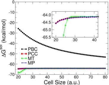
In Figs.1 and2, we report the behavior of the energy of a pyridine cation as a function of the cell size, for a system in periodic boundary conditions and for the different correc-tion schemes presented in the seccorrec-tions above, both without (Fig.1) and with (Fig.2) a continuum solvent as described by the SCCS method. As expected, both for the molecule in vacuum and for the solvated one, the periodic energy decays as the inverse power of the cell size, with a much less marked dependence for the solvated cases, due to the dielectric which screens the total charge and dipole moment of the system. Corrected results from the different methods are converged for cell sizes of 23 (27) a.u. for the vacuum (solvent) case, reflecting the larger size of the solvated system. The MP and PCC energies are found to converge as fast asL−5 (as seen in the log-log plot of the residual error, see Fig.4), while the Martyna-Tuckerman energies become constant and exact for cell sizes larger than 30 a.u. On the other hand, while for small cells the energies computed with the real-space approaches and the Makov-Payne are still less than 1 mRy away from the converged results, the Martyna-Tuckerman approach shows significant errors, even exceeding the uncorrected periodic energy. The same trend is reflected in the calculation of the electrostatic contribution to solvation free energies.
FIG. 1. (Color online) Total energy of a pyridine cation in vac-uum as a function of cell size, for PBC calculations and for the three correction schemes analyzed: Makov-Payne (MP, in blue), Martyna-Tuckerman (MT, in green), and point-countercharge (PCC in red).
FIG. 2. (Color online) Total energy of a pyridine cation in a dielectric medium as a function of cell size, for PBC calculations and for the three correction schemes analyzed: Makov-Payne (MP, in blue), Martyna-Tuckerman (MT, in green), and point-countercharge (PCC in red). For the dielectric medium, the SCCS parameters optimized to reproduce aqueous solvation of organic compounds, as derived in Ref. [13], have been used, but only the electrostatic contribution has been explicitly considered.
It is important to note that Makov-Payne energies are almost identical to the ones obtained with the self-consistent real-space approach. This validates the hypothesis, assumed by Makov and Payne, that the polarization of the charge density of the system due to periodic images affects only marginally its energy. The same behavior is true for solvated systems, with
FIG. 4. (Color online) Cell-size dependence of Makov-Payne (monopole and dipole+quadrupole) and polarization-specific (NCB and periodic) contributions to the energy. Reported decay exponents are estimated from fitting the large cell-size part of the figure. The residual error, after the different contributions have been subtracted from the total energy of the system, is shown to decay faster thanL−3 for cell sizes up to 40 a.u., while being negligible for larger cell sizes.
the Makov-Payne and the PCC methods almost exactly on top of each other.
Electrostatic solvation free energies, computed as the difference in total energy between the solvated and the vacuum case, are reported in Fig.3and substantially reflect what was found above: MP and PCC calculations give well-converged results (errors smaller than 0.5 kcal/mol) for all the system sizes considered, while the MT scheme gives large errors up to cell sizes of 26 a.u.
When looking at the different contributions to the Makov-Payne correction for a solvated system (Fig. 4), it appears that all contribute significantly. In particular, the effects of the
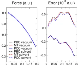
FIG. 5. (Color online) Hellmann-Feynman force (left panel) and error on forces (right panel) computed via finite differences for the nitrogen atom of the pyridine cation, in vacuum and in a continuum dielectric medium, with PBC or with MT and PCC correction schemes.
periodic images on polarizing the dielectric close to the solute are important, especially considering that, although small, such polarization is not charge neutral in the case of charged solutes. In order to validate the formulas derived and the imple-mentation of the different methods, the errors on the analytic forces have been reported in Fig.5for the different approaches considered as well as for the fully periodic case, with and without a continuum solvent. All the different methods show a very similar behavior, with errors almost three orders of magnitude smaller than the absolute value of the computed force. It is important to stress that, even though the reported errors are not negligible, all the methods are in agreement to what is found for the periodic calculations without the solvent,