Neural Networks

(1)

Rolf Pfeifer

Dana Damian

(2)

(3)

Introduction and motivation

The brain performs astonishing tasks: we can walk, talk, read, write, recognize hundreds of faces and objects, irrespective of distance, orientation and lighting conditions, we can drink from a cup, give a lecture, drive a car, do sports, we can take a course in neural networks at the university, and so on. Well, it’s actually not the brain, it’s entire humans that execute the tasks. The brain plays, of course, an essential role in this process, but it should be noted that the body itself, the morphology (the shape or the anatomy, the sensors, their position on the body), and the materials from which it is constructed also do a lot of useful work in intelligent behavior. The keyword here is embodiment, which is described in detail in [Pfeifer and Scheier, 1999] and [Pfeifer and Bongard, 2007]. In other words, the brain is always embedded into a physical system that interacts with the real world, and if we want to understand the function of the brain we must take embodiment into account.

Because the brain is so awesomly powerful, it seems natural to seek inspiration from the brain. In the field of neural computation (or neuro-informatics), the brain is viewed as performing computation and one tries to reproduce at least partially some of its amazing abilities. This type of computation is also called ”brain-style” computing.

One of the well-known interesting characteristics of brains is that the behavior of the individual neuron is clearly not considered ”intelligent” whereas the behavior of the brain as a whole is (again, we should also include the body in this argument). The technical term used here isemergence: if we are to understand the brain, we must understand how the global behavior of the brain-body system emerges from the activity and especially the interaction of many individual units.

In this course, we focus on the brain and the neural systems and we try to make proper abstractions so that we can not only improve our understanding of how natural brains function, but exploit brain-style computing for technological purposes. The termneural networks is often used as an umbrella term for all these activities.

Before digging into how this could actually be done, let us look at some areas where this kind of technology could be applied. In factory automation, number crunching, abstract symbol manipulation, or logical reasoning, it would not make sense because the standard methods of computing and control work extremely well, whereas for more ”natural” forms of behavior, such as perception, movement, lo-comotion, and object manipulation, we can expect interesting results. There are a number of additional impressive characteristics of brains that we will now look at anecdotally, i.e. it is not a systematic collection but again illustrates the power of natural brains. For all of these capacities, traditional computing has to date not come up with generally accepted solutions.

(6)

1. Some differences between computers and brains

Here are a few examples of differences between biological brains and computers. The point of this comparison is to show that we might indeed benefit by employing brain-style computation.

Parallelism. Computers function, in essence, in a sequential manner, whereas brains are massively parallel. Moreover, the individual neurons are densely con-nected to other neurons: a neuron has between just a few and 10,000 connections. Of particular interest is the observation that parallelism requires learning or some other developmental processes. In most cases it is not possible to either set the parameters (the weights, see later) of the network manually, or to derive them in a straightforward way by means of a formula: a learning process is required. The hu-man brain has roughly 1011_{neurons and 10}14_{synapses, whereas modern computers,}

even parallel supercomputers, typically – with some exceptions – have no more than 1000 parallel processors. In addition, the individual ”processing units” in the brain are relatively ”simple” and very slow, whereas the processing units of computers are extremely sophisticated and fast (cycle times in the range of nanoseconds).

This point is illustrated by the”100 step constraint”. If a subject in a reaction time task is asked to press a button as soon as he or she has recognized a letter, say ”A”, this lasts roughly 1/2s. If we assume that the ”operating cycle of a cognitive operation is on the order of 5-10ms, this yields a maximum of 200 operations per second. How is it possible that recognition can be achieved with only 200 cycles? The massive parallelism and the high connectivity of neural systems, as well as the fact that a lot of processing is performed right at the periphery (e.g. the retina), appear to be core factors.

Graceful degradation is a property of natural systems that modern computers lack to a large extent unless it is explicitly provided for. The term is used to designate systems that still operate - at least partially - if certain parts malfunction or if the situation changes in unexpected ways. Systems that display this property are

(a) noise and fault tolerant, and (b) they can generalize.

Noise tolerance means that if there is noise in the data or inside the system the function is not impaired, at least not significantly. The same holds for fault tolerance: If certain parts malfunction, the system does not grind to a halt, but continues to work - depending on the amount of damage, of course. The ability to generalize means that if there is a situation the system has never encountered before, the system can function appropriately based on its experience with similar situations. Generalization implies that similar inputs lead to similar outputs. In this sense, the parity function (of which the XOR is an instance) does not generalize (if you change only 1 bit at the input, you get maximum change at the out; see chapter 2). This point is especially important whenever we are dealing with the real world because there no two situations are ever identical. This implies that if we are to function in the real world, we must be able to generalize.

(7)

1. SOME DIFFERENCES BETWEEN COMPUTERS AND BRAINS 3

any intelligent system. There is a large literature on learning systems, traditional and with neural networks. Neural networks are particularly interesting learning systems because they are massively parallel and distributed. Along with the ability to learn goes the ability to forget. Natural systems do forget whereas computer don’t. Forgetting can, in a number of respects, be beneficial for the functioning of the organism: avoiding overload and unnecessary detail, generalization, forgetting undesirable experiences, focus on recent experiences, rather than on old ones, etc.

Learning always goes together with memory. The organization of memory in a computer is completely different from the one in the brain. Computer memories are accessed via addresses, there is a separation of program and data, and items once stored, are never forgotten, unless they are overwritten for some reason. Brains, by contrast, do not have ”addresses”, there is no separation of ”programs” and ”data”, and, as mentioned above, they have a tendency to forget. When natural brains search for memories, they use an organizational principle which is called ”associative memory” or ”content-addressable memory”: memories are accessed via part of the information searched for, not through an address. When asked what you had for lunch yesterday, you solve this problem by retrieving, for example, which class you attended before lunch, to which cafeteria you went etc., not by accessing a memory at a particular address (it is not even clear what an ”address” in the brain would mean).

Also, computers don’t ”get tired”, they function indefinitely, which is one of the important reasons why they are so incredibly useful. Natural brains get tired, they need to recover, and they occasionally need some sleep, learning.

Nonlinearity: Neurons are highly nonlinear, which is important particularly if the underlying physical mechanism responsible for the generation of the input signal is inherently (e.g. speech signal) nonlinear.

Recently, in many sciences, there has been an increasing interest in non-linear phenomena. If a system – an animal, a human, or a robot – is to cope with non-linearities, non-linear capacities are required. Many examples of such phenomena will be given throughout the class.

Plasticity: Learning and adaptivity are enabled by the enormous neural plas-ticity which is illustrated e.g. by the experiment of Melchner [von Melchner et al., 2000], in which the optic nerves of the eyes of a ferret were connected to the auditory cortex which then developed structures similar to the visual one.

The Paradox of the expert provides another illustration of the difference be-tween brains and computers. At a somewhat anecdotal level, the paradox of the expert is an intriguing phenomenon which has captured the attention of psychol-ogists and computer scientists alike. Traditional thinking suggests: the larger the database, i.e. the more comprehensive an individual’s knowledge, the longer it takes to retrieve one particular item. This is certainly the case for database sys-tems and knowledge-based syssys-tems no matter how clever the access mechanism. In human experts, the precise opposite seems to be the case: the more someone knows, the faster he or she can actually reproduce the required information. The paral-lelism and the high connectivity of natural neural systems are important factors underlying this amazing feat.

(8)

Figure 1. “tAe cHt”. The center symbol in both words is

iden-tical but, because of context, is read as an H in the first case and as an A in the second.

the center letter is identical for both words, but we naturally, without much reflec-tion, identify the one in the first word as an ”H”, and the one in the second word as an ”A”. The adjacent letters, which in this case form the context, provide the necessary constraints on the kinds of letters that are most likely to appear in this context. In understanding everyday natural language, context is also essential: if we understand the social situation in which an utterance is made, it is much easier to understand it, than out of context.

We could continue this list almost indefinitely. Because of the many favorable properties of natural brains, researchers in the field of neural networks have tried to harness some of them for the development of algorithms.

2. From biological to artificial neural networks

There are literally hundreds of textbooks on neural networks and we have no intention whatsoever of reproducing another such textbook here. What we would like to do is point out those types of neural networks that are essential for modeling intelligent behavior, in particular those which are relevant for autonomous agents, to systems that have to interact with the real world. The goal of this chapter is to provide an intuition rather than a lot of technical detail. The brain consists of roughly 1011 _{neurons. They are highly interconnected, each neuron making up}

to 10’000 connections, or synapses, with other neurons. This yields roughly 1014

synapses. The details do not matter here. We would simply like to communicate a flavor of the awesome complexity of the brain. In fact, it is often claimed that the human brain is the most complex known structure in the universe. More precisely, it’s the human organism which contains, as one of its parts, the brain.

Figure 2 (a) shows a model of a biological neuron in the brain. For our purposes we can ignore the physiological processes. The interested reader is referred to the excellent textbooks in the field (e.g. [Kandel et al., 1995]).

The main components of a biological neuron are the dendrites which have the task of transmitting activation from other neurons to the cell body of the neuron, which in turn has the task of summing incoming activation, and the axon which will transmit information, depending on the state of the cell body. The information on the cell body’s state is transmitted to other neurons via the axons by means of a so-called spike, i.e., an action potential which quickly propagates along an axon. The axon makes connections to other neurons. The dendrites can be excitatory, which means that they influence the activation level of a neuron positively, or they can be inhibitory in which case they potentially decrease the activity of a neuron. The impulses reaching the cell body (soma) from the dendrites arrive asynchronously at any point in time. If enough excitatory impulses arrive within a certain small time interval, the axon will send out signals in the form of spikes. These spikes can have varying frequencies.

(9)

2. FROM BIOLOGICAL TO ARTIFICIAL NEURAL NETWORKS 5

Figure 2. Natural and artificial neurons. Model of (a) a

biologi-cal neuron, (b) artificial neuron. The dendrites correspond to the connections between the cells, the synapses to the weights, the outputs to the axons. The computation is done in the cell body.

are discovered. If we want to develop models even of some small part of the brain we have to make significant abstractions. We now discuss some of them.

(10)

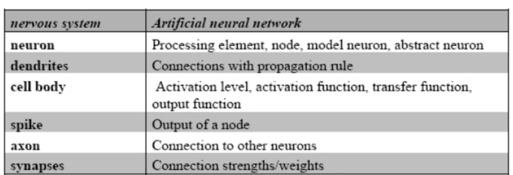
Figure 3. Natural and artificial neural networks

***where is the caption??***

employing this very abstract model or variations thereof. Table in Figure 3 shows the correspondences between the respective properties of real biological neurons in the nervous system and abstract neural networks.

Before going into the details of neural network models, let us just mention one point concerning the level of abstraction. In natural brains, there are many differ-ent types of neurons, depending on the degree of differdiffer-entiation, several hundred. Moreover, the spike is only one way in which information is transmitted from one neuron to the next, although it is a very important one. (e.g. [Kandel et al., 1991], [Churchland and Sejnowski, 1992]). Just as natural systems employ many different kinds of neurons and ways of communicating, there is a large vari-ety of abstract neurons in the neural network literature.

Given these properties of real biological neural networks we have to ask our-selves, how the brain achieves its impressive levels of performance on so many dif-ferent types of tasks. How can we achieveanythingusing such models as a basis for our endeavors? Since we are used to traditional sequential programming this is by no means obvious. In what follows we demonstrate how one might want to proceed. Often, the history of a field helps our understanding. The next section introduces the history of connectionism, a special direction within the field of artificial neural networks, concerned with modeling cognitive processes.

3. The history of connectionism

(11)

3. THE HISTORY OF CONNECTIONISM 7

Figure 4. Illustration of Rosenblatt’s perceptron. Stimuli

im-pinge on a retina of sensory units (left). Impulses are transmitted to a set of association cells, also called the projection area. This projection may be omitted in some models. The cells in the pro-jection area each receive a number of connections from the sensory units (a receptive field, centered around a sensory unit). They are binary threshold units. Between the projection area and the associ-ation area, connections are assumed to be random. The responses

Riare cells that receive input typically from a large number of cells in the association area. While the previous connections were feed-forward, the ones between the association area and the response cells are both ways. They are either excitatory, feeding back to the cells they originated from, or they are inhibitory to the com-plementary cells (the ones from which they do not receive signals). Although there are clear similarities to what is called a percep-tron in today’s neural network literature, the feedback connections between the response cells and the association are normally miss-ing.

Even though all the basic ideas were there, this research did not really take off until the 1980s. One of the reasons was the publication of Minsky and Papert’s seminal book ”Perceptrons” in 1969. They proved mathematically some intrinsic limitations of certain types of neural networks (e.g. [Minsky and Papert, 1969]). The limitations seemed so restrictive that, as a result, the symbolic approach began to look much more attractive and many researchers chose to pursue the symbolic route. The symbolic approach entirely dominated the scene until the early eighties; then problems with the symbolic approach started to come to the fore.

(12)

phenomenon has been found in the NETTalk model, a neural network that learns to pronounce English text (NETTalk will be discussed in chapter 3). After some period of learning, the network starts to behave as if it had learned the rules of English pronunciation, even though there were no rules in the network. So, for the first time, computer models were available that could do things the programmer had not directly programmed into them. The models had acquired their own his-tory! This is why connectionism, i.e. neural network modeling in cognitive science, still has somewhat of a mystical flavor.

Neural networks are now widely used beyond the field of cognitive science (see section 1.4). Applications abound in areas like physics, optimization, control, time series analysis, finance, signal processing, pattern recognition, and of course, neu-robiology. Moreover, since the mid-eighties when they started becoming popular, many mathematical results have been proved about them. An important one is their computational universality (see chapter 4). Another significant insight is the close link to statistical models (e.g. [Poggio and Girosi, 1990]). These results change the neural networks into something less mystical and less exotic, but no less useful and fascinating.

4. Directions and Applications

Of course, classifications are always arbitrary, but one can identify roughly four basic orientations in the field of neural networks, cognitive science/artificial intelli-gence, neurobiological modeling, general scientific modeling, and computer science which includes its applications to real-world problems. In cognitive science/artificial intelligence, the interest is in modeling intelligent behavior. This has been the fo-cus in the introduction given above. The interest in neural networks is mostly to overcome the problems and pitfalls of classical - symbolic - methods of modeling intelligence. This is where connectionism is to be located. Special attention has been devoted to phenomena of emergence, i.e. phenomena that are not contained in the individual neurons, but the network exhibits global behavioral patterns. We will see many examples of emergence as we go on. This field is characterized by a particular type of neural network, namely those working with activation levels. It is also the kind mostly used in applications in applied computer science. I is now common practice in the fields of artificial intelligence and robotics to apply insights from neuroscience to the modeling of intelligent behavior.

(13)

4. DIRECTIONS AND APPLICATIONS 9

Scientific modeling, of which neurobiological modeling is an instance, uses neu-ral networks as modeling tools. In physics, psychology, and sociology neuneu-ral net-works have been successfully applied. Computer science views neural netnet-works as an interesting class of algorithms that has properties –like noise and fault toler-ance, and generalization ability– that make them suited for application to real-world problems. Thus, the gamut is huge.

As pointed out, neural networks are now applied in many areas of science. Here are a few examples:

Optimization: Neural networks have been applied to almost any kind of op-timization problem. Conversely, neural network learning can often be conceived as an optimization problem in that it will minimize a kind of error function (see chapter 3).

Control: Many complex control problems have been solved by neural networks. They are especially popular for robot control: Not so much factory robots, but au-tonomous robots - like humanoids - that have to operate in real world environments that are characterized by higher levels of uncertainty and rapid change. Since bio-logical neural networks have evolved for precisely these kinds of conditions, they are well suited for such types of tasks. Also, because in the real world generalization is crucial, neural networks are often the tool of choice for systems, in particular robots, having interact with physical environments.

Signal processing: Neural networks have been used to distinguish mines from rocks using sonar signals, to detect sun eruptions, and to process speech signals. Speech processing techniques and statistical approaches involving hidden Markov models are sometimes combined.

Pattern recognition: Neural networks have been widely used for pattern recog-nition purposes, from face recogrecog-nition, to recogrecog-nition of tumors in various types of scans, to identification of plastic explosives in luggage of aircraft passengers (which yield a particular gamma radiation patterns when subjected to a stream of thermal neurons), to recognition of hand-written zip-codes.

Stock market prediction: The dream of every mathematician is to develop meth-ods for predicting the development of stock prices. Neural networks, in combination with other methods, are often used in this area. However, at this point in time, it is an open question whether they have been really successful, and if they have, the results wouldn’t have been published.

Classification problems: Any problem that can be couched in terms of classi-fication is a potential candidate for a neural network solution. Many have been mentioned already. Examples are: stock market prediction, pattern recognition, recognition of tumors, quality control (is the product good or bad), recognition of explosives in luggage, recognition of hand-written zip codes to automatically sort mail, and so on and so forth. Even automatic driving could be viewed as a kind of classification problem: Given a certain pattern of sensory input (e.g. from a camera, or a distance sensor), which is the best angle for the steering wheel, and the degree of pushing the accelerator or the brakes.

(14)

(15)

CHAPTER 2

Basic concepts

Although there is an enormous literature on neural networks and a very rich variety of networks, learning algorithms, architectures, and philosophies, a few underlying principles can be identified. All the rest consists of variations of these few basic principles. The ”four or five basics”, discussed here, provide such a simple framework. Once this is understood, it should present no problem to dig into the literature.

1. The four or five basics

For every artificial neural network we have to specify the following four or five basics. There are four basics that concern the network itself. The fifth one – equally important – is about how the neural network is connected to the real world, i.e. how it is embedded in the physical system. Embedded systems are connected to the real world through their own sensory and actuator systems. Because of their properties of robustness, neural networks are well-suited for such types of systems. Initially, we will mostly focus mostly on the computational properties (1) through (4) but later discuss complete embodied systems, in particular robots.

(1) The characteristics of the node. We use the terms nodes, units, processing elements, neurons, and artificial neurons synonymously. We have to define the way in which the node sums the inputs, how they are transformed into level of activation, how this level of activation is updated, and how it is transformed into an output which is transmitted along the axon.

(2) The connectivity. It must be specified which nodes are connected to which and in what direction.

(3) The propagation rule. It must be specified how a given activation that is traveling along an axon, is transmitted to the neurons to which it is connected.

(4) The learning rule. It must be specified how the strengths of the connec-tions between the neurons change over time.

(5) The fifth basic: embedding the network in the physical system: If we are interested in neural networks for embedded systems we must always spec-ify how the network is embedded, i.e. how it is connected to the sensors and the motor components.

In the neural network literature there are literally thousands of different kinds of network types and algorithms. All of them, in essence, are variations on these basic properties.

(16)

Figure 1. Node characteristics. ai: activation level,hi: summed weighted input into the node (from other nodes), oi: output of node (often identical withai),wij: weights connecting nodes j to node i (This is a mathematical convention used in Hertz, Krogh and Palmer, 1991; other textbooks use the reverse notation. Both notations are mathematically equivalent). ξi: inputs into the net-work, or outputs from other nodes. Moreover, with each node the following items are associated: an activation function g, transform-ing the summed inputhiinto the activation level, and a threshold, indicating the level of summed input required for the neuron to become active. The activation function can have various parame-ters.

2. Node characteristics

We have to specify how the incoming activation is summed, processed to yield level of activation, and how output is generated.

The standard way of calculating the level of activation of a neuron is as follows:

(1) ai=g(

n X

j=1

wijoj) =g(hi)

whereai is the level of activation of neuron i, oj the output of other neurons,

g the activation

function, hi the summed activation, and oi is the output. Normally we have

oi=f(ai) =ai , i.e., the output is taken to be the level of activation. In this case, equation (1) can be rewritten as

(2) ai=g(

n X

j=1

wijaj) =g(hi)

(17)

3. CONNECTIVITY 13

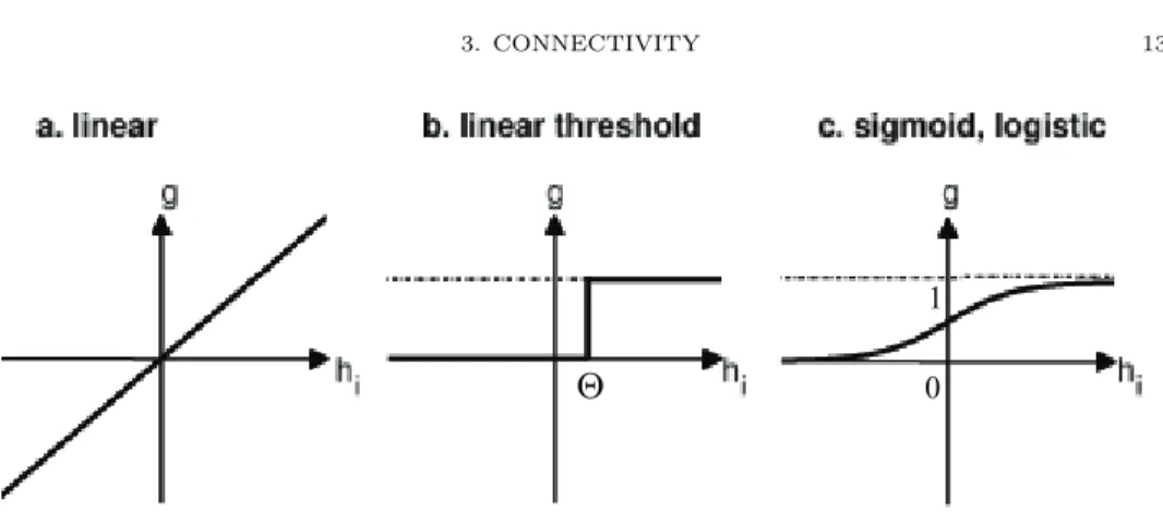
Figure 2. Most widely used activation functions. hi is the summed input,g the activation function. (a) linear function, (b) step function, (c) sigmoid function (also logistic function).

The sigmoid function is, in essence, a smooth version of a step function.

g(hi) = 1 1 +e−2βhi (3)

with β = 1/kBT (whereT can be understood as the absolute temperature). It is zero for low input. At some point it starts rising rapidly and then, at even higher levels of input, it saturates. This saturation property can be observed in nature where the firing rates of neurons are limited by biological factors. The slope, β

(also called gain) is an important parameter of the sigmoid function: The largerβ, the steeper the slope, the more closely it approximates the threshold function.

The sigmoid function varies between 0 and 1. Sometimes an activation function that varies between -1 and +1 with similar properties is required. This is the hyperbolic tangent:

tanh(x) = e x₋_e−x

ex₊_e₋x. (4)

The relation to the sigmoid functiong is given by tanh(βh) = 2g(h)−1. Because in the real world, there are no strict threshold functions, the ”rounded” versions – the sigmoid functions – are somewhat more realistic approximations of biological neurons (but they still represent substantial abstractions).

While these are the most frequently used activation functions, others are also used, e.g. in the case of radial basis functions which are discussed later. Radial basis function networks often use Gaussians as activation functions.

3. Connectivity

(18)

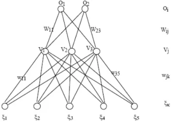
Figure 3. Graphical representation of a neural network. The connections are calledwij, meaning that this connection links node

jto nodeiwith weightwij(note that this is intuitively the ”wrong” direction, but it is just a notational convention, as pointed out earlier). The matrix representation for this network is shown in Figure 4

Figure 4. Matrix representation of a neural network

node 4 for ”straight”, and node 5 for ”turn right”. Note that nodes 1 and 3 are connected in both directions, whereas between nodes 1 and 4 the connection is only one-way. Connections in both directions can be used to implement some kind of short-term memory. Networks having connections in both directions are also called recurrent networks (see chapter 5). Nodes that have similar characteristics and are connected to other nodes in similar ways are sometimes called a layer. Nodes 1 and 2 receive input from outside the network; they are called theinput layer, while nodes 3, 4, and 5 form theoutput layer.

(19)

4. PROPAGATION RULE 15

Node 1 is not connected to itself (w11 = 0), but it is connected to nodes 3, 4, and 5 (with different strengths w31, w41, w51). The connection strength deter-mines how much activation is transferred from one node to the next. Positive connections are excitatory, negative ones inhibitory. Zeroes (0) mean that there is no connection. The numbers in this example are chosen arbitrarily. By analogy to biological neural networks, the connection strengths are sometimes also called synaptic strengths. The weights are typically adjusted gradually by means of a learning rule until they are capable of performing a particular task or optimize a particular function (see below). As in linear algebra the term vector is often used in neural network jargon. The values of the input nodes are often called theinput vector. In the example, the input vector might be (0.6 0.2) (the numbers have again been arbitrarily chosen). Similarly, the list of activation values of the output layer is called theoutput vector. Neural networks are often classified with respect to their connectivity. If the connectivity matrix has all zeroes in the diagonal and above the diagonal, we havefeed-forwardnetwork since in this case there are only forward connections, i.e., connections in one direction (no loops). A network with several layers connected in a forward way is called a multi-layer feed-forward network or multi-layer perceptron. The network in figure 3 is mostlyfeed-forward (connections only in one direction) but there is one loop in it (between nodes 1 and 3). Loops are important for the dynamical properties of the network. If all the nodes from one layer are connected to all the nodes of another layer we say that they arefully connected. Networks in which all nodes are connected to each other in both direc-tions but not to themselves are calledHopfield nets (Standard Hopfield nets also have symmetric weights, see later).

4. Propagation rule

We already mentioned that the weight determines how much activation is trans-mitted from one node to the next. The propagation rule determines how activation is propagated through the network. Normally, a weighted sum is assumed. For example, if we call the activation of node 4 a4 , we have a4 =a1w41+a2w42 or generally

(5) hi=

n X

j=1 wijaj

wherenis the number of nodes in the network,hi the summed input to node

i. hi is sometimes also called thelocal field of nodei. To be precise, we would have to useoj instead ofaj., but because the output of the node is nearly always taken to be its level of activation, this amounts to the same thing. This propagation rule is in fact so common that it is often not even mentioned. Note that there is an underlying assumption here, that activation transfer across the links takes exactly one unit of time. We want to make the propagation rule explicit because if - at some point - we intend to model neurons more realistically, we have to take the temporal properties of the propagation process such as delays into account.

(20)

Figure 5. Sigma-pi units

the intervals between the spikes. Moreover, traversing a link takes a certain amount of time and typically longer connections require more time to traverse. Normally, unless we are biologically interested, we assume synchronized networks where the time to traverse one link is one time step and at each time step the activation is propagated through the net according to formula 5.

Another kind of propagation rule uses multiplicative connections instead of summation only, as shown in formula 6 (see figure 5). Such units are also called sigma-pi units because they perform a kind of and/or computation. Units with summation only are called sigma units.

(6) hi=

X

wij Y

wikaj

There is a lot of work on dendritic trees demonstrating that complicated kinds of computation can already be performed at this level. Sigma-pi units are only a simple instance of them.

While conceptually and from a biological perspective it is obvious tha we have to specify the propagation rule, man textbooks do not deal with this issue explicitly – as mentioned, the one-step assumption is often implicitly adopted.

5. Learning rules

As already pointed out, weights are modified by learning rules. The learning rules determine how ”experiences” of a network exert their influence on its future behavior. There are, in essence, three types of learning rules: supervised, reinforce-ment, and non-supervised or unsupervised.

(21)

5. LEARNING RULES 17

Examples are the perceptron learning rule, the delta rule, and - most famous of all - backpropagation. Back-propagation is very powerful and there are many variations of it. The potential for applications is enormous, especially because such networks have been proved to be universal function approximators. Such learn-ing algorithms are used in the context of feedforward networks. Back-propagation requires a multi-layer network. Such networks have been used in many different areas, whenever a problem can be transformed into one of classification. A promi-nent example is the recognition of handwritten zip codes which can be applied to automatically sorting mail in a post office. Supervised networks will be discussed in great detail later on.

There is also a non-technical use of the word supervised. In a non-technical sense it means that the learning, say of children, is done under the supervision of a teacher who provides them with some guidance. This use of the term is very vague and hard to translate into concrete neural network algorithms.

5.2. Reinforcement learning. If the teacher only tells a student whether her answer is correct or not, but leaves the task of determining why the answer is correct or false to the student, we have an instance of reinforcement learning. The problem of attributing the error (or the success) to the right cause is called the credit assignment or blame assignment problem. It is fundamental to many learning theories. There is also a more technical meaning of the term of reinforcement learningas it is used in the neural network literature. It is used to designate learning where a particular behavior is to be reinforced. Typically, the robot receives a positive reinforcement signal if the result was good, no reinforcement or a negative reinforcement signal if it was bad. If the robot has managed to pick up an object, has found its way through a maze, or if it has managed to shoot the ball into the goal, it will get a positive reinforcement. Reinforcement learning is not tied to neural networks: there are many reinforcement learning algorithms in the field of machine learning in general. To use Andy Barto’s words, one of the champions of reinforcement learning ”Reinforcement learning [...] is a computational approach to learning whereby an agent tries to maximize the total amount of reward it receives when interacting with a complex, uncertain environment.”( [Sutton and Barto, 1998])

(22)

6. The fifth basic: embedding the network

(23)

CHAPTER 3

Simple perceptrons and adalines

1. Historical comments and introduction

This section introduces two basic kinds of learning machines from the class of supervised models: perceptrons and adalines. They are similar but differ in their activation function and as a consequence, in their learning capacity. We start with a historical comment, introduce classification, perceptron learning rules, adalines and delta rules.

2. The perceptron

The perceptron goes back to Rosenblatt (1958), as described in chapter 1. He formulated a learning algorithm, a way to systematically change the weights and proved its convergence, i.e. that after a finite number of steps, the perceptron would perform the desired computation. This generated a lot of enthusiasm in the community and there was the hope that machines would soon be capable of learning virtually anything.

There was, however, a limitation in Rosenblatt’s learning theorem, as pointed out by Marvin Minsky (one of the founders of the field of artificial intelligence) and Seymour Papert (the inventor of the ”Logo Turtles”), both mathematicians at MIT. They demonstrated in their book ”Perceptrons” that the theorem – obviously – only applies to those problems whose solutions can actually been computed. They showed that perceptrons could not perform some seemingly simple computations, a prominent example being the famous XOR problem: Given a network with two input nodes and one output node, if the input is zero and one, the output should be one, if both inputs are one or both are zero, the output should be zero.

In order to overcome the limitations, Rosenblatt also studied networks with several layers – which was the right intuition! However, at the time, there was no learning mechanism available to determine the weights to perform the desired com-putation. Because Minsky and Papert were skeptical about whether such learning schemes could be found, they and many others turned to symbol computation and the field of artificial intelligence turned into a discipline largely based on symbol processing. So, perceptrons, for a period of almost 20 years, largely disappeared from the scene. Still, a number of people continued working on perceptron-like or more generally network-like ideas.

But it was not until the 1980s when learning mechanisms were discovered that work in networks with multiple layers, the most famous of them being error back-propagation, e.g. by Rumelhart, Hinton and Williams in 1986 ( [Rumelhart et al., 1988]). Some people say that the learning algorithms had been re-discovered be-cause Werbos had published similar results already in 1974 ( [Werbos, 1974a]). However that may be, the availability of learning algorithms for multilayer networks

(24)

Figure 1. A perceptron with 4 input units and 3 output units.

Often the inputs and outputs are labeled with a pattern indexµ, and patterns typically range from 1 to p. Oµ_i is used to designate the actual output of the network. ζ_iµdesignates the desired output.

Figure 2. A simplified perceptron with only one output node.

led to a real explosion in the field of neural networks. Since then, neural networks have pervaded artificial intelligence, psychology, and the cognitive sciences.

2.1. The classification problem. Before we define the classification prob-lem, we need to introduce a bit of linear algebra (see also linear algebra tutorial).

Letξbe the input vector andgthe activation function (binary threshold) Figure 2 shows a simplified network with only one output node.

ξ= (ξ1, ξ2, . . . , ξn)T =                ξ1 ξ2 . . . . . . ξn               

g:O= 1,ifwTξ= n X

j=1

wjξj≥Θ

g:O= 0,ifwTξ= n X

j=1

wjξj<Θ

wTξ: scalar product, inner product (7)

(25)

2. THE PERCEPTRON 21

Ω = Ω1∪Ω2

ξin Ω1 : O should be 1 (true)

ξin Ω2 : O should be 0 (false) (alternatively it could be−1)

Alternatively – and also often used in the literature – the desired output should be -1. We will be using both notations as we go along.

Learning goal: Learn separation such that for eachξ in Ω1

Pn

j=1wjξj ≥Θ and for eachξ in Ω2

Pn

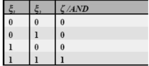
j=1wjξj <Θ Example: AND problem

Let us look at a very simple example, the AND problem. Ω1={(1,1)} →1

Ω2 = {(0,0),(0,1),(1,0)} → 0 Learning goal: The network should learn to

produce a 1 at its output if the input vector is (1,1) and 0 if it is (0,0),(0,1), or (1,0). If the output is correct, we don’t change anything. If it is incorrect we have to distinguish two cases, i.e. O = 1, but should be 0, and O = 0 but should be 1. Let’s try to get an intuition of the perceptron learning rule by looking at how thresholds and weights have to be changed:

1. Thresholds:

O=1, should be 0: Θ→increase O=0, should be 1: Θ→decrease

2. Weights: O=1, should be 0: ifξi= 0→no change ifξi= 1→decreasewi O=0, should be 1: ifξi= 0→no change ifξi= 1→increasewi Trick:

ξ→(−1, ξ1, ξ2, . . . , ξn)

w→(Θ, w1, w2, . . . , wn)

Notation: (ξ0, ξ1, ξ2, . . . , ξn); (w0, w1, w2, . . . , wn)

2.2. Perceptron learning rule. Since most of the knowledge in a neural network is contained in the weights, learning means systematically changing the weights. There are also learning schemes where other parameters (e.g. the gain of the activation function) are changed – we will look at a few examples later in the course, but for now, we focus on weight change.

ξ in Ω1

ifwTξ≥0→OK ifwTξ <0

(26)

Figure 3. Truth table for the AND function

ξ in Ω2

ifwTξ≥0

w(t) =w(t−1)−ηξ wi(t) =wi(t−1)−ηξi

ifwTξ <0→OK (9)

Formulas (8 and 9) are a compact way of writing the perceptron learning rule. It includes the thresholds as well as the weights.

Example: i= 0→w0 is threshold

w0(t) =w0(t−1) +ηξ0→ −Θ(t) =−Θ(t−1) +η1 →Θ(t) = Θ(t−1)−η1

(reduction).

The question we then immediately have to ask is under what conditions this learning rule converges. The answer is provided by the famous perceptron conver-gence theorem:

2.3. Perceptron convergence theorem. The algorithm with the percep-tron learning rule terminates after a finite number of iterations with constant in-crement (e.g. η = 1), if there is a weight vectorw∗ which separates both classes (i.e. if there is a configuration of weights for which the classification is correct). The next question then is when such a weight vector w∗ exists. The answer is that the classes have to be linearly separable. So, we always have to distinguish clearly between what can be represented and what can be learned (and under what conditions). The fact that something can be represented, e.g. a weight vector that separates the two categories exists, does not necessarily imply that it can also be found by a learning procedure.

Linear separability means that a plane (or if we are talking about high-dimensional spaces, a hyperplane) can be found in theξ-space separating the patterns in Ω1for

which the desired value is +1, and the patterns in Ω2 for which the desired value

is 0. If there are several output units, such a plane must be found for each output unit. The truth table for the AND function is shown in figure 3.

It is straightforward to formulate the inequalities for the AND problem. Fig. 4 depicts a simple perceptron representing the AND function together with a rep-resentation of the input space. The line separating Ω1 and Ω2 in 2D input space is

given by the equation

w1ξ1+w2ξ2=θ

(27)

2. THE PERCEPTRON 23

Figure 4. A simple perceptron. A possible solution to the AND

problem is shown. There is an infinite number of solutions.

Figure 5. Truth table for the XOR function

which implies

ξ2= θ w2 −

w1 w2ξ1.

(11)

This is the usual form of the equation for a liney=b+ax with slopeaand offset b.

And then do the same for the XOR problem (figure 5). As you will see, this latter problem is not linearly separable, in other words, there is no way to satisfy all the inequalities by proper choice ofθ, w1 andw2.

Pseudocode for the perceptron algorithm:

Select random weightswat time t=0.

.REPEAT

.Select a random patternξfrom Ω1∪Ω2,t=t+1; . IF(ξfrom Ω1)

. THEN IFwT_{ξ <}₀

. THENw(t) =w(t−1) +ηξ . ELSEw(t) =w(t−1)→OK

. ELSE IFwTξ≥0

. THENw(t) =w(t−1)−ηξ . ELSEw(t) =w(t−1)

.UNTIL(allξhave been classified correctly)

There are a number of proofs of the perceptron convergence theorem in the literature, for example

(28)

is referred to these publications.

3. Adalines

The Adaline, the Adaptive Linear Element, is very similar to the perceptron: it’s also a one-layer feedforward network, the only difference is the activation func-tion at the output, which is linear instead of a step funcfunc-tion.

Linear units:

O_iµ=P_jwijξjµ

which implies thatO_iµ is continuous. As usual, the desired output isOµ_i =ζ_iµ

One advantage of continuous units is that a cost function can be defined. Cost is defined in term of the error, E(w). This implies that optimization techniques (like gradient methods) can be applied.

3.1. Delta learning rule. Remember that in the perceptron learning rule the factor ηξ only depends on the input vector and not on the size of the error (because the output is either correct or not). The delta rule takes the size of the error into account.

∆wij =−η(Oiµ−ζ µ i)ξ

µ j =−ηδ

µ iξ

µ

j, withδ µ i = (O

µ i −ζ

µ i) (12)

This formula is also called the Adaline rule (Adaline=Adaptive linear element) or the Widrow-Hoff rule. If the input is large, the corresponding weights contribute more to the error than if the input is small. In other words, this rule solves the blame assignment problem, i.e. which weights contribute most to the error (and thus need to be changed most by the learning rule). The delta rule implements an LMS procedure (LMS=least mean square), as will be shown, below. Let us define a cost function or error function:

E(w) =1 2

X

µ X

i

(O_iµ−ζ_iµ)2= 1 2 X µ X i (X j

wijξµj −ζ µ i) 2 = 1 2 X µ,i (X j

wijξµj −ζ µ i)

2

(13)

where i is the index of the output units and µ runs over all patterns. The better our choice ofw’s for a given set of input patterns, the smallerEwill be. E

depends on the weights and on the inputs.

Consider now the weight space (in contrast to the state space which is con-cerned with the activation levels).

(29)

3. ADALINES 25

∆wij=−η

∂E ∂wij (14)

We can also write the vector notation

∆w=−η∇E(w) (15)

where the Nabla operator∇indicates the gradient:

∇E(w) =

∂E ∂w1,

∂E ∂w2, . . . ,

∂E ∂wn

(16)

The intuition is that we should change the weights in the direction where the error gets smaller the fastest - this is precisely the opposite of the gradient (−∇) in this error function. Using the chain rule and considering that wij is the only weight which is not ”constant” for this operation (which implies that many terms drop out), we get

−η ∂E ∂wij

=−ηX

µ

(O_iµ−ζ_iµ)ξ_jµ

If we consider one single patternµ:

∆w_ijµ =−η(Oµ_i −ζ_iµ)ξ_jµ=−ηδ_iµξ_jµ

which corresponds to the delta rule. In other words the delta rule realizes a gradient descent procedure in the error function.

3.2. Explicit Solution: (The mathematics of this and the next section is not subject to the final examination. What is important here are the conditions under which solutions exist or can be explicitly calculated in the general case, as well as the generalized delta rule for non-linear units.) In some cases, we can cal-culate the weights explicitly, i.e. without the need of an iterative learning procedure:

wij= 1

N

X

µ,ν

ζ_iµ(Q−1)µνξjν,where

Qµν = 1

N

X

j

ξµ_jξ_jν

(17)

Qµν only depends on the input patterns. Note that we can only calculate the weights in this manner if Q−1 _{exists. This condition requires that the input}

patterns be linearly independent. Linear independence means that there is no set of patternsai where not allai = 0,such that

a1ξj1+a2ξ

2

j+. . .+apξ p

j = 0, ∀j (18)

(30)

the outputs cannot be chosen independently and then the problem can normally not be solved.

Note thatlinear independencefor linear (and non-linear) units is distinct fromlinear separability defined for threshold units (in the case of the classical perceptron). Linear independence implies linear separability, but the reverse is not true. In fact, most of the problems of interest in neural networks do not satisfy the linear independence condition, because the number of patterns is typically larger than the number of dimensions of the input space (i.e. the number of input nodes), i.e.

p > N. If the number of vectors is larger than the dimension, they are always linearly dependent.

3.3. Existence of solution. Again, we have to ask ourselves when a solution exists. The question ”Does a solution exist” means: Is there a set of weights wij such that all the ξµ can be learned such that the actual output is equal to the desired output? ”Can be learned” means:

Oµ_i =ζ_iµ,∀ξµ

In other words, the actual output of the network is equal to the desired output for all the patternsξµ.

Linear units:

For linear units this is the same as saying:

ζ_iµ =X j

wijξjµ,∀ξ µ

Since Adalines use linear units, the Oµ_i are continuous-valued, which is an advan-tage over the Perceptron which has only binary output. Still Adalines can only find a solution for classification tasks if the input classes arelinearly separable.

Non-linear units:

For non-linear units we have to generalize the delta rule, because the latter has been defined for linear units only. This is straightforward. We explain it here because we will need it in the next chapter when introducing the backpropagation learning algorithm.

Assume thatgis the standard sigmoid activation function:

g(h) = [1 + exp(−2βh)]−1₌ 1 1+e−2βh

Note that g is continuously differentiable, which is a necessary property for the generalized delta rule to be applicable.

The error function is:

E(w) = 1 2

X

i,µ

(Oµ_i −ζ_iµ)2= 1 2

X

i,µ

[g(hµ_i)−ζ_iµ]2

hµ_i =X j

(31)

3. ADALINES 27

In order to calculate the weight change we form the gradient, just as in the linear case, using the chain rule:

∆wij=−η

∂E ∂wij

∂E(w)

∂wij

=X µ

[g(hµ_i)−ζ_iµ]g0(hµ_i)ξ_jµ=X µ

δ_iµξµ_j

δ= [g(hµ_i)−ζ_iµ]g0(hµ_i) ∆wij =−η

X

µ

δµ_iξ_jµ or for a single pattern: ∆w_ijµ =−ηδµ_iξ_jµ

(20)

This generalized delta rule now simply contains the derivative of the activation functiong0. Because of the specific mathematical form, these derivatives are par-ticularly simple:

g(h) = [1 +exp(−2βh)]−1

g0(h) = 2βg(1−g) (21)

forβ =1 2 →g

0₍_h_{) =}_g₍₁₋_g₎

We will make use of these relationships in the actual algorithms for back-propagation.

With non-linear activation functions we can finally solve nonlinear problems, so they do not have to be linearly separable anymore. The existence of a solution however, is always different from the question whether a solutioncan be found. We will not go into the details here, but simply mention that in the non-linear case there may be local minima in the error function, whereas in the linear case the global minimum can always be found. The capacity of one-layer perceptrons to represent functions is limited. As long as we have linear units, adding additional layers does not extend the capacity of the network. However if we have non-linear units, the networks become in factuniversal function approximators (see next chapter).

3.4. Terminology. Before going on to discuss multi-layer perecpetrons, we need to introduce a bit of terminology.

Cycle: 1 pattern presentation, propagate activation through network, change weights Epoch: 1 ”round” of cycles through all the patterns

Error surface: The surface spanned by the error function, plotted in weight space. Given a particular set of patternsξµ to be learned, we have to choose the weights such that the overall error becomes minimal. The error surface visualizes this idea. The learning process can then be viewed as a trajectory on the error surface (see figure 5 in chapter 4).

If the weights are updated only at the end of an epoch, we have the following learning rule which sums over all patternsµ:

∆wij =−η X

µ

δ_iµξ_jµ

(22)

(32)

(23) ∆w_ijµ =−ηδ_iµξ_jµ

(23) is called the on-line version. Here, the weights are updated after each pattern presentation. In this case the order in which the patterns are presented to the network matters.

(33)

CHAPTER 4

Multilayer perceptrons and backpropagation

Multilayer feed-forward networks, or multilayer perceptrons (MLPs) have one or several ”hidden” layers of nodes. This implies that they have two or more layers of weights. The limitations of simple perceptrons do not apply to MLPs. In fact, as we will see later, a network with just one hidden layer can represent any Boolean function (including the XOR which is, as we saw, not linearly separable). Although the power of MLPs to represent functions has been recognized a long time ago, only since a learning algorithm for MLPs, backpropagation, has become available, have these kinds of networks attracted a lot of attention. Also, on the theoretical side, the fact that it has been proved in 1989 that, loosely speaking, MLPs are universal function approximators [Hornik et al., 1989], has added to their visibility (but see also section 4.6).

1. The back-propagation algorithm

The back-propagation algorithm is central to much current work on learning in neural networks. It was independently invented several times (e.g. [Bryson and HO, 1969,Werbos, 1974b,Rumelhart et al., 1986b,Rumelhart et al., 1986a])

As usual, the patterns are labeled byµ, so input k is set toξ_kµ when pattern

µ is presented. The ξ_kµ can be binary (0,1) or continuous-valued. As always, N

Figure 1. A two-layer perceptron showing the notation for units and weights.

(34)

designates the number of input units,pthe number of input patterns (µ=1, 2, . . . ,

p).

For an input patternµ, the input to nodej in the hidden layer (the V-layer) is

hµ_j =X k

wjkξ µ k (24)

and the activation of the hidden nodeV_jµ becomes

V_jµ=g(hµ_j) =g(X k

wjkξ_kµ) (25)

whereg is the sigmoid activation function. Output uniti(O-layer) gets

hµ_i =X j

WijV µ j =

X

j

Wijg( X

k

wjkξ µ k) (26)

and passing it through the activation functiong we get:

Oµ_i =g(hµ_i) =g(X j

WijV µ j ) =g(

X

j

Wijg( X

k

wjkξ µ k)) (27)

Thresholds have been omitted. They can be taken care of by adding an extra input unit, the bias node, connecting it to all the nodes in the network and clamping it’s value to (-1); the weights from this unit represent the thresholds of each unit.

The error function is again defined for all the output units and all the patterns:

E(w) =1 2

X

µ,i

[Oµ_i −ζ_iµ]2= 1 2

X

µ,i [g(X

j

WijV µ j )−ζ

µ i] 2 = 1 2 X µ,i [g(X

j

Wijg( X

k

wjkξ_kµ))−ζiµ]

2

(28)

Because this is a continuous and differentiable function of every weight we can use a gradient descent algorithm to learn appropriate weights:

∆Wij =−η

∂E ∂Wij

=−ηX

µ

[O_iµ−ζ_iµ]g0(hµ_i)V_jµ=−ηX

µ

δµ_iV_jµ

(29)

withδ_iµ= [Oµ_i −ζ_iµ]g0(hµ_i) To derive (29) we have used the following relation:

∂ ∂Wij

g(X j

Wijg( X

k

wjkξkµ)) =g0(h µ i)V

µ j

W11V

µ

1 +W122

µ

1 +. . .+WijV µ j +. . . (30)

Because the W11 etc. are all constant for the purpose of this differentiation, the respective derivatives are all 0, except forWij.

(35)

1. THE BACK-PROPAGATION ALGORITHM 31

∂WijVjµ

∂Wij

=V_jµ

As noted in the last chapter, for sigmoid functions the derivatives are particu-larly simple:

g0(hµ_i) =Oµ_i(1−O_iµ)

δ_iη= (O_iµ−ζ_iµ)Oµ_i(1−O_iµ) (31)

In other words, the derivative can be calculated from the function values only (no derivatives in the formula any longer)!

Thus for the weight changes from the hidden layer to the output layer we have:

∆Wij =−η

∂E ∂Wij

=−ηX

µ

δ_iµV_jµ=−ηX

µ

(Oµ_i −ζ_iµ)O_iµ(1−O_iµ)V_jµ

(32)

Note thatg no longer appears in this formula.

In order to get the derivatives of the weights from input to hidden layer we have to apply the chain rule:

∆wjk =−η

∂E ∂wjk

=−η ∂E ∂V_jµ

∂V_jµ ∂wjk after a number of steps we get:

∆wjk=−η X

µ

δ_jµξµ_k

whereδ_jµ= (X i

Wijδiµ)g0(h µ j) = (

X

i

Wijδµi)V µ j (1−V

µ j ) (33)

And here is the complete algorithm for backpropagation:

Naming conventions:

m: index for layer M: number of layers m = 0: input layer

V0

i =ξi ; weightwijm: V m₋1

j toV m i ;ζ

µ

i : desired output (1) Initialize weights to small random numbers.

(2) Choose a pattern ξ_kµ from the training set; apply to input layer (m=0)

V_k0=ξ_kµ for all k

(3) Propagate the activation through the network:

Vm

i =g(hmi ) =g( P

jw m ijV

m−1

j ) for all i andm until all VM

i have been calculated (V M

(36)

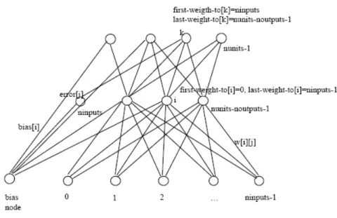
Figure 2. Illustration of the notation for the backpropagation algorithm.

(4) Compute the deltas for the output layer M:

δM

i =g0(hMi )[ζ µ i −V

M i ],

for sogmoid: δ_iM =V_iM(1−V iM)[ζ_iµ−V_iM]

(5) Compute the deltas for the preceding layers by successively propagating the errors backwards

δ_im−1=g0(h_im−1)P_jw_jimδm_j

for m=M, M-1, M-2, . . . , 2 until a delta has been calculated for every unit.

(6) Use ∆wm

ij =ηδimV m−1

j

to update all connections according to (*)wnew

ij =wijold+ ∆wij

(7) Go back to step 2 and repeat for the next pattern.

Remember the distinction between the ”on-line” and the ”off-line” version. This is the on-line version because in step 6 the weights are changed after each individual pattern has been processed (*). In the off-line version, the weights are changed only once all the patterns have been processed, i.e. (*) is executed only at the end of an epoch. As before, only in the online version the order of the patterns matters.

2. Java-code for back-propagation

Figure 2 demonstrates the naming conventions in the actual Java-code. This is only one possibility - as always there are many ways in which this can be done. Shortcuts:

(37)

2. JAVA-CODE FOR BACK-PROPAGATION 33

Variables

first weight to[i]Index of the first node to which node i is connected last weight to[i]Index of last node to which node i is connected bias[i] Weight vector from bias node

netinput[i] Total input to node i activation[i] Activation of node i logistic Sigmoid activation function weight[i][j] Weight matrix

nunits Number of units (nodes) in the net ninputs Number of input units (nodes) noutputs Number of output units (nodes) error[i] Error at node i

target[i] Desired output of node i

delta[i] error[i]*activation[i]*(1-activation[i]) wed[i][j] Weight error derivatives

bed[i] Analog wed for bias node eta Learning rate

momentum (a) Reduces heavy oscillation activation[] Input vector

1. Calculate activation

.

.compute output () {

. for (i = ninputs; i < nunits; i++) {

. netinput[i] = bias [i];

. for (j=first weight to[i]; j<last weight to[i]; j++) {

. netinput[i] += activation[j]*weight[i][j];

. }

. activation[i] = logistic(netinput[i]);

. }

.} .

2. Calculate ”error”

”t” is the index for the target vector (desired output);

”activation[i]*(1.0 - activation[i])” is the derivative of the sigmoid acti-vation function (the ”logistic” function)

The last ”for”-loop in compute erroris the ”heart” of the backpropagation algo-rithm: the recursive calculation of error and delta for the hidden layers. The program iterates backwards through all nodes, starting with the last output node. For every passage through the loop, thedelta is calculated by multiplyingerror

with the derivative of the activation function. Then,deltagoes back to the nodes (multiplied with the connection weightweight[i][j]). If then a specific node be-comes the actual node (index ”i”), the sum (error) is already accumulated, i.e. all the contributions of the nodes to which the actual node is projecting are already considered. delta is then again calculated by multiplying error with the deriva-tive of the activation function:

(38)

g0= activation[i] * (1 - activation[1])

.

.compute error() {

. for (i = ninputs; i < nunits - noutputs; i++) {

. error[i] = 0.0;

. }

. for (i = nunits - noutputs, t=0; i<nunits; t++, i++) {

. error[i] = target[t] - activation[i];

. }

. for (i = nunits - 1; i >= ninputs; i--) {

. delta[i] = error[i]*activation[i]*(1.0 - activation[i]); // (g’)

. for (j=first weight to[i]; j < last weight to[i]; j++)

. error[j] += delta[i] * weight[i][j];

. }

.} .

3. Calculating wed[i][j]

wed[i][j](”weight error derivative”) isdelta of nodeimultiplied with the activation of the node to which it is connected byweight[i][j]. Connections from nodes with a higher level of activation contribute a bigger part to error correction (blame assignment).

.

.compute wed() {

. for (j=first weight to[i]; j<last weight to[i]; j++) {

. wed[i][j] += delta[i]*activation[j];

. }

. bed[i] += delta[i];

. }

.} .

4. Update weights

In this procedure the weights are changed by the algorithm. In this version of backpropagation a momentum term is used.

.

.change weights () {