Qiu_unc_0153D_19322.pdf

(1)

CHARACTERIZING RESPONSES OF LAND SURFACE PHENOLOGY TO URBANIZATION, CLIMATE CHANGE, AND EXTREME WEATHER EVENTS USING

(2)

(3)

ABSTRACT

Tong Qiu: Characterizing response of land surface phenology to urbanization, climate change, and extreme weather events using remote sensing and Bayesian models

(under the direction of Dr. Conghe Song)

Land surface phenology (LSP) is the intra-annual rhythm of vegetation dynamic from dormancy to activity and back to dormancy over the landscape. Shifts of LSP have cascading effects on food production, carbon sequestration, water consumption, biodiversity, and public health. There are three major knowledge gaps in understanding the impacts of urbanization, climate change, and extreme weather events on LSP. (1) Previous studies mainly focused on investigating the effects of urbanization on the spatial patterns of LSP by comparing the phenological metrics between urban center and the surrounding rural regions. However, it remains unclear how urbanization-induced land cover conversions and climate change jointly influence the temporal variations of LSP. (2) Conventional methods usually model key

phenological transition dates (e.g. discrete timing of spring bud-break and fall senescence) based on aggregated climate variables (e.g. mean temperature, growing-degree days), ignoring the fact that LSP is a dynamic and continuous process which responds to daily weather conditions continuously. (3) Current projection of LSP shifts under future environmental changes relies heavily on species-level observations and degree-day models. It is challenging to produce a set of future LSP metrics in a temporally consistent manner at regional-to-continental scales.

(4)

(5)

(6)

ACKOWLEDGEMENTS

The past five years for my Ph.D. study at UNC-Chapel Hill has been a wonderful journey for me. The academic environment here allows me to freely pursued new ideas and developed new models with so many amazing minds around. Among them the most important is my

(7)

(8)

TABLE OF CONTENTS

TABLE OF CONTENTS ... viii

LIST OF TABLES ... xii

LIST OF FIGURES ... xv

CHAPTER ONE:INTRODUCTION ... 1

CHAPTER TWO: SPATIO-TEMPORAL VARIATIONS OF LAND SURFACE PHENOLOGY AND THEIR RESPONSES TO URBANIZATION AND CLIMATE CHANGE ... 9

2.1 Introduction ... 9

2.1.1 Understanding impacts of urbanization on spatial variation of land surface phenology requires fine-spatial resolution remote sensing ... 9

2.1.2 Joint effects of climate change and urbanization on temporal shift of land surface phenology remain less studied ... 12

2.2 Study Sites and Data ... 14

2.2.1 Understanding spatial variation of LSP in Shanghai China ... 14

2.2.2 Understanding temporal variation of LSP in 196 large cities ... 16

2.3 Methods ... 19

2.3.1 Understanding impacts of landscape configuration and composition on urban phenology ... 19

2.3.1.1 Deriving Landsat-scale land surface phenology ... 19

2.3.1.2 Deriving Landscape metrics ... 22

2.3.2 Separating impacts of urbanization from that of climate change on temporal changes of land surface phenology ... 24

(9)

2.3.1.2 Deriving land surface phenology from VIPv4 ... 27

2.3.1.3 Characterizing impacts of climate change ... 30

2.3.1.4 Statistical analysis ... 31

2.4 Results ... 32

2.4.1 Spatial variations of land surface phenology and their relationships with landscape metrics along the rural-urban-rural transect in Shanghai, China ... 32

2.4.1 Temporal variations of land surface phenology and their relationships with climate change and urbanization in 196 large cities ... 41

2.5 Discussion ... 48

2.5.1 impacts of landscape metrics on land surface phenology ... 48

2.5.2 Individual effects of urbanization and climate change on the temporal shifts of land surface phenology ... 51

CHAPTER THREE:UNDERSTANDING THE CONTINUOUS PHENOLOGICAL DEVELOPMENT AT DAILY TIME STEP WITH A BAYESIAN HIERARCHICAL SPACE-TIME MODEL: IMPACTS OF CLIMATE CHANGE AND EXTREME WEATHER EVENTS ... 59

3.2 Materials and methods ... 63

3.2.1 Dataset ... 63

3.2.1.1 VIP4 EVI2 dataset ... 63

3.2.1.2 ESA’s Land cover dataset ... 64

3.2.1.3 Daymet dataset ... 65

3.2.2 Study site ... 65

3.2.3 Preprocessing daily EVI2 time series ... 66

3.2.4 Bayesian Hierarchical Space-Time Model for Land surface phenology (BHST-LSP) ... 68

(10)

3.2.4.2 Model covariates ... 71

3.2.4.3 Model implementation and validation ... 73

3.3 Results ... 76

3.3.1 Performance of the BHST-LSP model ... 76

3.3.2 Spatial pattern of sensitivity of speed of LSP to rate of climate covariates ... 81

3.3.3 Sensitivity of speed of LSP to rate of climate covariates in different land cover types ... 90

3.4.1 Impacts of temperature on the continuous phenological development ... 95

3.4.2 Impacts of water on the continuous phenological development ... 99

3.4.3 BHST-LSP Model performance and opportunity for future improvement ... 101

CHAPTER FOUR:PROJECTING LAND SURFACE PHENOLOGY FROM 2020 TO 2099 IN THE CONTERMINOUS UNITED STATES ... 104

4.2 Data ... 107

4.2.1 Remote Sensing dataset ... 107

4.2.2 Climate dataset ... 108

4.3 Methods ... 109

4.3.1 Deriving historical and future LSP ... 109

4.3.2 Statistical Analysis ... 111

4.4 Results ... 112

4.4.1 Performance of BHST-LSP in estimating historical LSP ... 112

4.4.2 Future shifts of LSP and pre-season climate conditions ... 115

(11)

APPENDIX ... 137

Supplementary materials to chapter two ... 137

Supplementary materials to chapter three ... 153

Supplementary materials to chapter four ... 168

(12)

LIST OF TABLES

Table 2. 1 Percentages of LCLU types in 2.5-m spatial resolution classification

map. ... 16 Table 2. 2 Eight Köopen-Geiger climate zones and their brief descriptions

(Alvares et al. 2013). The table also summarized the number of cities

within each climate zone. ... 17 Table 2. 3 Multi-season images used for LCLU classification with the AASG

algorithm. The images for the year 1995 were classified separately and its

LCLU map was used as reference map for AASG. ... 21 Table 2. 4 Landscape pattern metrics used in this study, after McGarigal et al.

(2012). ... 23 Table 2. 5 Pearson correlation coefficients between SOS, EOS, and LOS of urban

vegetation and class level landscape metrics for time intervals 1984–1995, 1996–2000, and 2001–2005. The last two letters after each landscape

metric signify the LCLU type as defined in table 2.1 ... 36 Table 2. 6 Pearson correlation coefficients between SOS, EOS, and LOS of urban

vegetation and class level landscape metrics for time intervals 1984–1995, 1996–2000, and 2001–2005. The last two letters after each landscape

metric signify the LCLU type as defined in Section 2.2. ... 38 Table 2. 7 Regression coefficients from the multiple linear regression for the

effects of urbanization and climate change on the shifts of start of season (SOS) and end of season (EOS) across eight climate zones. The predictor variables of SOS are changes in growing degree days ( GDD),

accumulated precipitation ( AP), accumulated insolation ( AS), and amplitude of urbanization ( %ISA) between post- and pre-urbanization time period. The predictor variables of EOS are differences of chilling degree days ( CDD), AP, AS, and %ISA from pre- to

post-urbanization time period. The significance of each coefficients was tested with a 2-tailed test (*** means p-value<0.001, ** means p-value<0.01. * means p-value<0.05). It should be noted that for coefficients without stars, they are all significant at 0.1 level (p-value<0.1). R2_{represents the}

coefficient of determination for the multiple regression. The R2_{for each of} MLR analysis across the climate zones are all significant at 0.001 level (2-tailed test). Description of climate zone symbols are provided in Table 2.2. Number of 0.05˚ pixels used in the MLR analysis for each climate zone

(13)

Table 3. 1 Covariates used in this study ... 73 Table A2. 1 Descriptions of 196 cities used in this study. The first column is the

“ISOURBID”, which provide a unique ID for each city. This table also included the name, geographical location (latitude and longitude, i.e. centroids of polygons from GRUMPv1 dataset), and total population of

each city ... 137 Table A2. 2 Ten Phenocam sites used to verify the derived land surface

phenology. Note that VIPv4 dataset ended at year 2014. There were thus

total 31 site-years for validation in this study. ... 142 Table A2. 3 Regression coefficients from the multiple linear regression. The

predictor variables of SOS are changes in growing degree days ( GDD), accumulated precipitation ( AP), accumulated insolation ( AS), and amplitude of urbanization ( %ISA) between post- and pre-urbanization time period as well as %ISA in the pre-urbanization period. The predictor variables of EOS are differences of chilling degree days ( CDD), AP,

AS, and %ISA from pre- to post-urbanization time period as well as %ISA in the pre-urbanization period. The significance of each

coefficients was tested with a 2-tailed test (*** means p-value<0.001, ** means p-value<0.01. * means p-value<0.05). Description of climate zone

symbols are provided in Table 2.2. ... 143 Table A2. 4 Detailed p-values for the regression coefficients from the multiple

linear regression (Table A2.3) for the effects of %ISA in the pre-urbanization period on the shifts of start of season (SOS) and end of season (EOS) across eight climate zones. Description of climate zone

symbols are provided in Table 2.2. ... 144 Table A2. 5 The effects of urbanization and climate change on the shifts of start

of season (SOS) and end of season (EOS) in terms of partial correlation coefficient across different climate zones. The coefficients were tested with a 2-tailed test (*** means p-value<0.001, ** means p-value<0.01. * means p-value<0.05). All coefficients without stars are significant at 0.1

level (p-value<0.1). ... 144 Table A3. 1 The reliable layer of the VIP dataset and their associated weights.

We gave weight of 1 to the excellent and good quality data. The acceptable and marginal data has a weight of 0.5. For the rest of the

rankings, we gave a low weight of 0.2 ... 156 Table A3. 2 we randomly selected 6 ecoregions that has more than 750 pixels,

(14)

remaining data to validate the model, the results for the spring season were

summarized in the table below. ... 161 Table A3. 3 we randomly selected 6 ecoregions that has more than 750 pixels,

and utilized the 10%, 20%, 30%, 40%, 50% of the data to train while the remaining data to validate the model, the results for the fall season were

summarized in the table below. ... 163 Table A4. 1 The z-value and adjusted p-value from the Dunn's test. Diff1

corresponds to shifts of LSP metrics between future time interval 2021-2040 and historical baseline 1981-2000; Diff2 corresponds to shifts of LSP metrics between future time interval 2051-2070 and historical baseline 1981-2000; Diff3 corresponds to shifts of LSP metrics between future time

(15)

LIST OF FIGURES

Figure 2. 1 (a) The location of Shanghai in China. (b) Administrative boundary of

Shanghai and the east-west transect. ... 14 Figure 2. 2 Spatial distributions of 196 large cities selected in this study and their

corresponding climate zones. Each point on the map represents one city. The size of the point is proportional to the population. The abbreviations of

climate zones can be found in Table 2.2. ... 17 Figure 2. 3 Three typical examples of the temporal trajectory of the annual

percentage of impervious surface area (%ISA). Dotted line is the raw time series of %ISA. Solid line represents the fitted time series. (a) an example of urban growth from non-urban to low-density urban (%ISA between 0.2 and 0.49) at 47.925˚N, 37.825˚E (Donetsk, Ukraine); (b) an example of urban growth from non-urban to moderate-density urban (%ISA between 0.49 and 0.8) at 40.625˚N, 109.975˚E (Baotou, China); (c) an example of urban growth from low-density urban to moderate-density urban at 45.725˚N, 126.525˚E

(Harbin, China). ... 26 Figure 2. 4 Spatial pattern of mean SOS for urban vegetation along the east-west

(d) 2006–2010 and (e) 2011–2015. ... 33 Figure 2. 5 Spatial pattern of mean EOS for urban vegetation along the east-west

(d) 2006–2010 and (e) 2011–2015. ... 33 Figure 2. 6 Spatial pattern of mean LOS for urban vegetation along the east-west

(d) 2006–2010 and (e) 2011–2015. ... 34 Figure 2. 7 Spatial mean SOS (a); EOS (b) and LOS (c) for urban vegetation as a

function of distance along the east-west transect that runs through the urban center. The columns represent the periods: 1984–1995, 1996–2000, 2001– 2005, 2006–2010, and 2011–2015. Bold lines represented average SOS, EOS, and LOS and shaded areas represented ± one standard deviation within

each 5 km blocks. ... 35 Figure 2. 8 Spatial patterns of the amplitude of urbanization for each city. Each

point represents the city-level zonal mean of differences of percentage of impervious surface area ( %ISA) between the post- and the pre-urbanization

time period. ... 42 Figure 2. 9 Spatial patterns of changes from pre- to post-urbanization for each city.

(16)

growing degree days ( GDD); (c) changes in spring pre-season accumulated precipitation ( AP); (d) changes in spring pre-season accumulated insolation

( AS). ... 43 Figure 2. 10 Spatial patterns of changes from pre- to post-urbanization for each city.

Each point represents the city-level zonal level mean values. Specifically, (a) changes in the end of season ( EOS); (b) changes in fall pre-season chilling degree days ( CDD); (c) changes in fall pre-season accumulated

precipitation ( AP); (d) changes in fall pre-season accumulated insolation

( AS). ... 44 Figure 3. 1 The Study sites and their dominant land cover types. Each polygon in

this map denotes the boundaries for the EPA's Level IV ecoregions. The dominant land cover with each ecoregion is shown in the map with different

colors. ... 66 Figure 3. 2 Accuracy assessment of the BHST-LSP model for spring phenology

based on the three metrics (a) R2, (b) NRMSE, and (c) rBIAS. Purple polygon boundaries pointed out the 295 ecoregions where in-sample metrics (i.e. models were calibrated and validated using the same dataset) were used to evaluate the model. The other 619 ecoregions used out-of-sample metrics (i.e. models were calibrated using train dataset and were validated using test dataset, respectively). The breaks of the color legend were selected to ensure

that there were similar number of ecoregions within each color categories. ... 77 Figure 3. 3 Accuracy assessment of the BHST-LSP model for fall phenology based

on the three metrics (a) R2, (b) NRMSE, and (c) rBIAS. Purple polygon boundaries pointed out the 295 ecoregions where in-sample metrics (i.e. models were calibrated and validated using the same dataset) were used to evaluate the model. The other 619 ecoregions used out-of-sample metrics (i.e. models were calibrated using train dataset and were validated using test dataset, respectively). The breaks of the color legend are the same as Figure 3.2 to ensure that we can compare the performance of BHST-LSP between

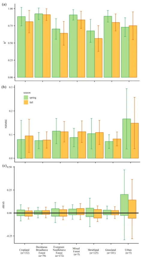
spring and fall phenology. ... 78 Figure 3. 4 The mean and standard deviation (i.e. marked by the error bar, note that

positive and negative rBIAS are calculated separately) of the out-of-sample metrics of (a) R2_{, (b) NRMSE, and (c) rBIAS for spring and fall phenology} across the seven land cover types in the 619 ecoregions. The number of eco-regions that had the out-of-sample metrics were also labeled for each of the 7

land covers. ... 79 Figure 3. 5 The sensitivity of speed of spring phenology to the changing rates of (a)

(17)

covariate is not significant in that eco-region (the 95% Bayesian posterior

credible interval contains zero). ... 82 Figure 3. 6 The sensitivity of speed of fall phenology to the changing rates of (a)

daily maximum temperature anomaly (b) daily minimum temperature anomaly across the 914 ecoregions in the CONUS. The breaks of the color legend were selected to ensure that there were similar number of ecoregions within each color categories. Purple polygon boundary pointed out that the covariate is not significant in that eco-region (the 95% Bayesian posterior

credible interval contains zero). ... 83 Figure 3. 7 The sensitivity of rate of spring phenology to the changing rate of (a)

frost events (b) hot events across the 914 ecoregions in the CONUS. The breaks of the color legend were selected to ensure that there were similar number of ecoregions within each color categories. Purple polygon boundary pointed out that the covariate is not significant in that eco-region (the 95%

Bayesian posterior credible interval contains zero). ... 85 Figure 3. 8 The sensitivity of speed of fall phenology to the changing rate of (a) frost

events (b) hot events across the 914 ecoregions in the CONUS. The breaks of the color legend were selected to ensure that there were similar number of ecoregions within each color categories. Purple polygon boundary pointed out that the covariate is not significant in that eco-region (the 95% Bayesian

posterior credible interval contains zero). ... 86 Figure 3. 9 The sensitivity of rate of spring phenology to the changing rate of (a)

accumulated precipitation (b) heavy rainfall events across the 914 ecoregions in the CONUS. The breaks of the color legend were selected to ensure that there were similar number of ecoregions within each color categories. Purple polygon boundary pointed out that the covariate is not significant in that

eco-region (the 95% Bayesian posterior credible interval contains zero). ... 88 Figure 3. 10 The sensitivity of speed of fall phenology to the changing rate of (a)

accumulated precipitation (b) heavy rainfall events (c) drought events across the 914 ecoregions in the CONUS. The breaks of the color legend were selected to ensure that there were similar number of ecoregions within each color categories. Purple polygon boundary pointed out that the covariate is not significant in that eco-region (the 95% Bayesian posterior credible

interval contains zero). ... 89 Figure 3. 11 The percentage of positive (bars above 0) and negative (bars below 0)

for the coefficients (i.e. Bayesian posterior median of sensitivity of speed of LSP to rate of climate covariates) across the seven land cover types for the spring phenology (a) and fall phenology (b), respectively. The colored bars indicated that the coefficient is significant (the 95% Bayesian posterior credible interval did not contain zero). The number of ecoregions is also

(18)

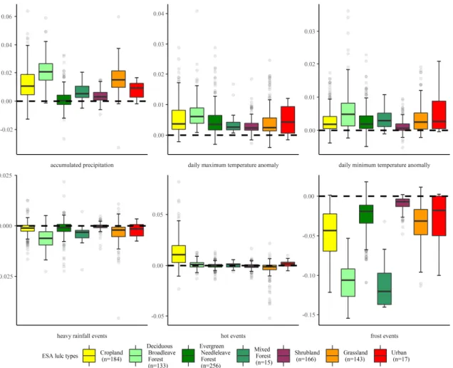
Figure 3. 12 The coefficient (i.e. Bayesian posterior median of sensitivity of speed of LSP to rate of climate covariates) for the spring season summarized by the

boxplot across different land cover types. ... 93 Figure 3. 13 The coefficient (i.e. Bayesian posterior median of sensitivity of speed

of LSP to rate of climate covariates) for the fall season summarized by the

boxplot across different land cover types. ... 94 Figure 3. 14 The proportion of coefficients of daily maximum (day-time) and

minimum (night-time) temperature under the four different scenarios (i.e. max temperature + and min temperature +, max temperature + and min temperature –, max temperature – and min temperature +, max temperature – and min temperature – where + means positive coefficient, that is, faster increase in temperature will advance rate of spring phenology and – means negative coefficient, that is, faster increase in temperature will delay speed of spring phenology) as well as the comparison in their magnitudes (i.e. absolute values). Colored bars indicate different scenarios. The transparency of the colored bar represents whether the absolute value of the coefficient of maximum temperature is higher than that of the minimum temperature (i.e.

high transparency) or not (low transparency). ... 97 Figure 3. 15 The proportion of coefficients of daily maximum (day-time) and

minimum (night-time) temperature under the four different scenarios (i.e. max temperature + and min temperature +, max temperature + and min temperature –, max temperature – and min temperature +, max temperature – and min temperature – where + means positive coefficient, that is, slower decrease in temperature will delay rate of fall phenology and – means negative coefficient, that is, slower decrease in temperature will advance speed of fall phenology) as well as the comparison in their magnitudes (i.e. absolute values). Colored bars indicate different scenarios. The transparency of the colored bar represents whether the absolute value of the coefficient of maximum temperature is higher than that of the minimum temperature (i.e.

high transparency) or not (low transparency). ... 98 Figure 4. 1 The boxplot (i.e. middle bar indicates the median value, lower and upper

hinges marked the 25th_{and 75}th_{of percentiles) of the out-of-sample metrics} RMSE for spring and fall phenology across the seven land cover types in the

619 ecoregions. ... 113 Figure 4. 2 The absolute difference in days (modeled – observed) across the

CONUS for spring (a) and fall (b) phenology, respectively. Note that both in-sample LSP and out-of-in-sample were used to calculate the ecoregion level mean and then subtract the observed LSP. The differences are also the mean

values from 1981 to 2014. ... 114 Figure 4. 3 The shifts of start of season between the three future periods

(19)

for two climate projection scenarios (RCP 4.5 and RCP 8.5). The first columns (a, c, and e) represents the RCP 4.5 scenario while the second columns (b, d, f) marks the RCP 8.5 scenarios. All six panels share the common legend so that we can directly compared the differences in the SOS shifts. (a) and (b) represents the difference between the future time interval 2021-2040 and historical baselines 1981-2000; (c) and (d) are similar to (a)

and (b) but for the future time interval 2051-2070; (e) and (f) for 2081-2099. ... 119 Figure 4. 4 The histograms for shifts of start of season for the three future periods

(2021-2040, 2051-2070, and 2081-2099) from the historical baselines

(1981-2000) for RCP 4.5 climate projection scenario. ... 120 Figure 4. 5 The histograms for shifts of start of season for the three future periods

(1981-2000) for RCP 8.5 climate projection scenario. ... 120 Figure 4. 6 The shifts of end of season between the three future periods (2021-2040,

2051-2070, and 2081-2099) from the historical baselines (1981-2000) for two climate projection scenarios (RCP 4.5 and RCP 8.5). The first columns (a, c, and e) represents the RCP 4.5 scenario while the second columns (b, d, f) marks the RCP 8.5 scenarios. All six panels share the common legend so that we can directly compared the differences in the SOS shifts. (a) and (b)

represents the difference between the future time interval 2021-2040 and historical baselines 1981-2000; (c) and (d) are similar to (a) and (b) but for

the future time interval 2051-2070; (e) and (f) for 2081-2099. ... 121 Figure 4. 8 The histograms for shifts of start of season for the three future periods

(1981-2000) for RCP 8.5 climate projection scenario. ... 122 Figure 4. 7 The histograms for shifts of start of season for the three future periods

(1981-2000) for RCP 4.5 climate projection scenario. ... 122 Figure 4. 9 The changes of spring pre-season mean max temperature between the

three future periods (2021-2040, 2051-2070, and 2081-2099) from the historical baselines (1981-2000) for two climate projection scenarios (RCP 4.5 and RCP 8.5). The first columns (a, c, and e) represents the RCP 4.5 scenario while the second columns (b, d, f) marks the RCP 8.5 scenarios. All six panels share the common legend so that we can directly compared the differences in the SOS shifts. (a) and (b) represents the difference between the future time interval 2021-2040 and historical baselines 1981-2000; (c) and (d) are similar to (a) and (b) but for the future time interval 2051-2070;

(e) and (f) for 2081-2099. ... 123 Figure 4. 10 The changes of spring pre-season accumulated precipitation between

(20)

historical baselines (1981-2000) for two climate projection scenarios (RCP 4.5 and RCP 8.5). The first columns (a, c, and e) represents the RCP 4.5 scenario while the second columns (b, d, f) marks the RCP 8.5 scenarios. All six panels share the common legend so that we can directly compared the differences in the SOS shifts. (a) and (b) represents the difference between the future time interval 2021-2040 and historical baselines 1981-2000; (c) and (d) are similar to (a) and (b) but for the future time interval 2051-2070;

(e) and (f) for 2081-2099. ... 124 Figure 4. 11 The changes of fall pre-season mean max temperature between the

(e) and (f) for 2081-2099. ... 125 Figure 4. 12 The changes of fall pre-season accumulated precipitation between the

(e) and (f) for 2081-2099. ... 126 Figure 4. 13 The box plot (i.e. middle bar indicates the median value, lower and

upper hinges marked the 25th_{and 75}th_{of percentiles) for different land cover} types regarding to their shifts of start of season between the three future periods (2021-2040, 2051-2070, and 2081-2099) and the historical baselines

(1981-2000) for both RCP 4.5 and RCP 8.5 climate projection scenarios. ... 131 Figure 4. 14 The box plot (i.e. middle bar indicates the median value, lower and

upper hinges marked the 25th_{and 75}th_{of percentiles) for different land cover} types regarding to their shifts of start of season between the three future periods (2021-2040, 2051-2070, and 2081-2099) and the historical baselines

(1981-2000) for both RCP 4.5 and RCP 8.5 climate projection scenarios. ... 131 Figure A2. 1 Comparison between the ISA derived from ESA's CCI Land cover

dataset and Landsat-base urban maps, respectively. Each point represents the city-level zonal mean. Each color indicates one of the eight climate zones.

(21)

Figure A2. 2 The comparison of temporal consistencies between ESA CCI’s land cover dataset and Landsat-based urban maps within the random selected 0.05 grids across 36 cities (labeled by the ISOURBID). Red dots represent the Landsat %ISA in years of 1995, 2000, 2005, 2010, and 2015, respectively. Dashed line represents the raw ESA’s CCI %ISA time series. Solid line shows the fitted %ISA. Blue and green points are the starting and ending

years of urbanization, respectively ... 146 Figure A2. 3 Comparison of start of season (SOS) and end of season (EOS) derived

from PhenoCam and VIP dataset. They grey dashed line indicate the 1:1 line. The grey solid line shows the simple linear regression line. Different color

points represent phenological metrics derived at different site. ... 147 Figure A2. 4 Spatial patterns of spring (a) pre-season base temperature for growing

degree days (GDD) calculation; (b) pre-season length of GDD; (c) pre-season length of accumulated precipitation (AP); and (d) pre-season length of

accumulated insolation (AS). Each point represents city-level zonal mean. ... 148 Figure A2. 5 Bar plot of pre-season base temperature for GDD calculations across

eight climate zones ... 149 Figure A2. 6 Bar plot of pre-season length of SOS for growing degree days (GDD),

accumulated precipitation (AP), and accumulated insolation (AS) across eight

climate zones ... 149 Figure A2. 7 Spatial patterns of fall (a) pre-season base temperature for chilling

degree days (CDD) calculation; (b) pre-season length of CDD; (c) pre-season length of accumulated precipitation (AP); and (d) pre-season length of

accumulated insolation (AS). Each point represents city-level zonal mean. ... 150 Figure A2. 8 Bar plot of the pre-season base temperature for the calculation of

chilling degree days (CDD) across eight climate zones ... 151 Figure A2. 9 Bar plot of pre-season length of EOS for chilling degree days (CDD),

accumulated precipitation (AP), and accumulated insolation (AS) across eight

climate zones ... 151 Figure A2. 10 Spatial patterns of shits of length of season (LOS). Each point

represents the city-level zonal mean. ... 152 Figure A2. 11 Proportion of urban grids with potential multiple urban growth

periods. Each point represents the city-level zonal mean. ... 152 Figure A3. 1 The original and the Whittaker filtered time series for randomly

selected pixels for each of the seven land cover types (their locations can be found in Figure A3.4). (a) cropland pixel, (b) deciduous broadleaf forest (c) evergreen needleleaf forest, (d) mixed forest, (e) shrubland, (f) grassland, (g)

(22)

Figure A3. 2 The “optimal” time intervals preceding the given day in which the highest correlations occurred between vegetation greenness and the climate covariates, i.e. (a) accumulated precipitation, (b) hot events, (c) frost events,

and (d) heavy rainfall events, for the spring season ... 158 Figure A3. 3 The “optimal” time intervals preceding the given day in which the

highest correlations occurred between vegetation greenness and the climate covariate, i.e. (a) accumulated precipitation, (b) hot events, (c) frost events,

(d) heavy rainfall events, and (e) drought events, for the fall season ... 159 Figure A3. 4 The 6 ecoregions and their dominant land cover types that we used to

test if lower proportion of training data and higher proportion of testing data will affect our proposed BHST-LSP model performance. We also labeled the

random selected pixel locations for Figure A3.1 ... 160 Figure A3. 5 Accuracy assessment of the BHST-LSP model for spring phenology

based on the three metrics in-sample metrics (the validation data is also the training data, it is a measurement for goodness of fit) (a) R2, (b) NRMSE, and (c) rBIAS for the 914 ecoregions. The breaks of the color legend were selected to ensure that there were similar number of ecoregions within each

color categories. ... 165 Figure A3. 6 Accuracy assessment of the BHST-LSP model for fall phenology

based on the three metrics in-sample metrics (the validation data is also the training data, it is a measurement for goodness of fit) (a) R2_{, (b) NRMSE, and} (c) rBIAS for the 914 ecoregions. The breaks of the color legend are the same as Figure A3.5 to ensure that we can visually compare the performance of

BHST-LSP between spring and fall phenology. ... 166 Figure A3. 7 The mean and standard deviation (i.e. marked by the error bar, note

that positive and negative rBIAS are calculated separately) of the in-sample metrics of (a) R2_{, (b) NRMSE, and (c) rBIAS for spring and fall phenology} across the seven land cover types in the 619 ecoregions. The number of eco-regions that had the out-of-sample metrics were also labeled for each of the 7

land covers. ... 167 Figure A4. 1 The boxplot (i.e. middle bar indicates the median value, lower and

upper hinges marked the 25th_{and 75}th_{of percentiles) of the in-sample metrics} RMSE for spring and fall phenology across the seven land cover types in the 619 ecoregions. The number of eco-regions that had the in-sample metrics

were also labeled for each of the 7 land covers. ... 168 Figure A4. 2 The absolute difference in days (modeled – observed) for each

individual year from 1981 to 2014 across the CONUS for spring phenology. Note that both in-sample LSP and out-of-sample were used to calculate the

(23)

Figure A4. 3 The absolute difference in days (modeled – observed) for each individual year from 1981 to 2014 across the CONUS for fall phenology. Note that both in-sample LSP and out-of-sample were used to calculate the

ecoregion level mean and then subtract the observed LSP. ... 170 Figure A4. 4The changes of spring pre-season mean min temperature between the

(e) and (f) for 2081-2099. ... 172 Figure A4. 5The changes of fall pre-season mean minimum temperature between the

(e) and (f) for 2081-2099. ... 173 Figure A4. 6The changes of pre-season heat events for spring phenology between

the three future periods (2021-2040, 2051-2070, and 2081-2099) from the historical baselines (1981-2000) for two climate projection scenarios (RCP 4.5 and RCP 8.5). The first columns (a, c, and e) represents the RCP 4.5 scenario while the second columns (b, d, f) marks the RCP 8.5 scenarios. All six panels share the common legend so that we can directly compared the differences in the SOS shifts. (a) and (b) represents the difference between the future time interval 2021-2040 and historical baselines 1981-2000; (c) and (d) are similar to (a) and (b) but for the future time interval 2051-2070;

(e) and (f) for 2081-2099. ... 174 Figure A4. 7 The changes of pre-season heat events for fall phenology between the

(24)

and (d) are similar to (a) and (b) but for the future time interval 2051-2070;

(e) and (f) for 2081-2099. ... 175 Figure A4. 8 The changes of pre-season frost events for spring phenology between

the three future periods (2021-2040, 2051-2070, and 2081-2099) from the historical baselines (1981-2000) for two climate projection scenarios (RCP 4.5 and RCP 8.5). The first columns (a, c, and e) represents the RCP 4.5 scenario while the second columns (b, d, f) marks the RCP 8.5 scenarios. All six panels share the common legend so that we can directly compared the differences in the SOS shifts. (a) and (b) represents the difference between the future time interval 2021-2040 and historical baselines 1981-2000; (c) and (d) are similar to (a) and (b) but for the future time interval 2051-2070;

(e) and (f) for 2081-2099. ... 176 Figure A4. 9 The changes of pre-season frost events for fall phenology between the

(e) and (f) for 2081-2099. ... 177 Figure A4. 10 The changes of pre-season heavy rainfall events for spring phenology

between the three future periods (2021-2040, 2051-2070, and 2081-2099) from the historical baselines (1981-2000) for two climate projection scenarios (RCP 4.5 and RCP 8.5). The first columns (a, c, and e) represents the RCP 4.5 scenario while the second columns (b, d, f) marks the RCP 8.5 scenarios. All six panels share the common legend so that we can directly compared the differences in the SOS shifts. (a) and (b) represents the difference between the future time interval 2021-2040 and historical baselines 1981-2000; (c) and (d) are similar to (a) and (b) but for the future time interval 2051-2070;

(e) and (f) for 2081-2099. ... 178 Figure A4. 11 The changes of pre-season heavy rainfall events for fall phenology

between the three future periods (2021-2040, 2051-2070, and 2081-2099) from the historical baselines (1981-2000) for two climate projection scenarios (RCP 4.5 and RCP 8.5). The first columns (a, c, and e) represents the RCP 4.5 scenario while the second columns (b, d, f) marks the RCP 8.5 scenarios. All six panels share the common legend so that we can directly compared the differences in the SOS shifts. (a) and (b) represents the difference between the future time interval 2021-2040 and historical baselines 1981-2000; (c) and (d) are similar to (a) and (b) but for the future time interval 2051-2070;

(25)

Figure A4. 12 The changes of pre-season drought events for spring phenology between the three future periods (2021-2040, 2051-2070, and 2081-2099) from the historical baselines (1981-2000) for two climate projection scenarios (RCP 4.5 and RCP 8.5). The first columns (a, c, and e) represents the RCP 4.5 scenario while the second columns (b, d, f) marks the RCP 8.5 scenarios. All six panels share the common legend so that we can directly compared the differences in the SOS shifts. (a) and (b) represents the difference between the future time interval 2021-2040 and historical baselines 1981-2000; (c) and (d) are similar to (a) and (b) but for the future time interval 2051-2070;

(26)

CHAPTER 1 INTRODUCTION

Land surface phenology (LSP), the interannual rhythm of the start, progress and ending of vegetation growth, is widely used as an indicator of ecological effects from urbanization and climate change (Buyantuyev and Wu 2012; Neil and Wu 2006; Richardson et al. 2013). Although cities only occupy a small proportion (with a continental average of 0.5%) of global land surface (Schneider et al. 2009), urbanization profoundly affects local-to-continental terrestrial ecosystem processes and services (Foley et al. 2005; Grimm et al. 2008; Seto et al. 2012). The surface urban heat island (sUHI) effects (Oke 1973; Voogt and Oke 2003) amplify the global warming trends, shifting vegetation phenology and leaving urban ecosystems increasingly vulnerable to heat-related problems. Vegetation provides crucial ecosystem services, such as regulating local climate, producing food, serving as habitats for wildlife, and promoting human well-being. It is critical to understand how urbanization and climate change-induced changes of LSP affect those ecosystem services. LSP is highly sensitive to interannual variability in climate, but it can also in turn influence the climate itself (Richardson et al. 2013). An accurate knowledge of urbanization and climate change effects on LSP can thus help better modeling climate and developing mitigation and adaptation strategies for the adversary

(27)

LSP of vegetation has the potential to affect the population dynamics of higher tropic levels, especially for avian species (Miller-Rushing et al. 2010; Thackeray et al. 2016). Therefore, quantifying LSP changes can provide insights on phenology mismatch at different trophic levels, enabling more effective conservation of biodiversity. Furthermore, because LSP determines the periods of pollen production and the allergy seasons (Neil and Wu 2006), investigating

phenological shifts can thus provide important information for public health practitioners to provide timely public health services.

Remote sensing provides consistent, objective, and quantitative measurements of Earth surface properties in a repetitive manner, making satellite images ideal resources for deriving LSP. (de Beurs and Henebry 2004). Many algorithms have been developed to extract LSP based on time series of vegetation indices from Advanced Very High Resolution Radiometer

(28)

the sUHI effects on LSP within a very localized range (Oke 1973). These confounding effects at local scales cannot be detected by AVHRR and MODIS. The opening of the Landsat archive and its free data access policy (Woodcock et al. 2008) have enabled the pixel-wise long-term time series analyses at finer spatial resolution (30 × 30 m). But there still exists the fundamental challenge when monitoring LSP using remote sensing, which is the inherent trade-off between spatial resolution and revisit time provided by the images. Data from AVHRR and MODIS blurs the spatial details in LSP, but they cover the land surface in a high-frequency. Landsat, on the other hand, provide sufficient spatial detail but have revisit time that is too sparse to capture annual vegetation phenological dynamics. More Landsat-based model need to be developed to estimate LSP in cities. Additionally, the impacts from landscape metrics on the spatial pattern of Landsat-based LSP in the urban ecossytem remains little studied. There are thus unrealized potentials for leveraging Landsat images to derive LSP and better understand the relationship between spatial patterns of LSP and landscape configuration and composition spanning multi-decadal time scales. As for the temporal shifts of LSP, they are highly responsive to long-term changes in climate (e.g. global warming trends, changes in the timing and amount of rainfall, drought- and heat-related stresses) (Richardson et al. 2013). The impacts of climate change on LSP has been extensively studied in both temperature- and precipitation-controlled ecosystems. But few studies have considered the impacts of urbanization-induced land cover change (i.e. the increases of fractions of impervious surface area) on LSP. Urban vegetation is documented to experience larger phenological shifts compared with its rural counterpart since these

anthropogenic effects have changed urban climatic conditions. However, knowledge gaps still exist in how urbanization-induced environmental changes act and interact with climate

(29)

(30)

validated using National Phenology Network (NPN) (Melaas et al. 2016a) and other ground-based observation datasets (Chuine et al. 1998, 1999) to investigate how weather and climate variations influence spring phenology. However, Clark et al., 2014a and 2014b argued that models based on degree-days might be problematic to understand warming effects from climate change on discrete phenological events of spring onset. Those models use highly aggregated variables (i.e. degree days) which collapse daily temperature into a cumulative number for an entire year or season based on a set of thresholds (Clark et al. 2014a). In doing so, those models overlook the fact that daily vegetation growth could respond to daily temperature continuously (Clark et al. 2014b). The thresholds in those models are also difficult to identify (Terres et al. 2013), especially when time series of temperature is highly fluctuating (Chuine et al. 1998). Additionally, current models did not allow process errors and observation errors. To address those limitations, Clark et al., 2014a and 2014b developed a continuous development model (CDM) that accommodated the inconsistency between the discrete observations of phenological events and continuous responses of vegetation phenology to temperature using a hierarchical state-space model (Clark et al. 2011). As for fall phenology, most published studies reported that its possible environmental drivers include summer temperature, precipitation and photoperiod. Delpierre et al. (2009) modeled fall phenology through a chilling degree-days photoperiod-dependent model using 400 leaf coloring data from deciduous trees acquired in France during the period of 1997-2006. They concluded the delays in leaf coloring were correlated with increases in late summer or early fall temperatures. Archetti et al. (2013) applied a similar model in a New England forest and reported that fall phenology models should be improved by including

(31)

using data from Harvard Forest and evaluated the model based on USA NPN network. They found the sensitivity of fall senescence to temperature is nonlinear, with warmer regions having a larger sensitivity than that in cooler regions. However, some studies point out different results. Estrella and Menzel (2006) used Pearson’s correlation to investigate the associations between meteorological conditions and fall senescence in deciduous trees. They concluded there is no significant correlations between fall phenology and those environmental drivers. Menzel et al. (2008) also attributed the delays of fall senescence to high temperatures in late spring instead of summer season using a Bayesian analysis. As changes in timing of fall senescence plays a significant role in growing season length, C and N cycling, and biotic interactions (Gallinat et al. 2015), more efforts should be made to understand which environmental drivers influence fall phenology.

These lacks of knowledge and inconsistencies in finding have motivated this dissertation here. Specifically, chapter 2 aimed to explore the spatial-temporal variation of LSP and their responses to climate change and urbanization by answering the following three questions: (1) How does vegetation phenology vary spatially along a rural-to-urban transect over the past three decades? (2) How do landscape composition and configuration affect those spatial variations of vegetation phenology? (3) How do SOS and EOS vary before and after urbanization? (4) How much of those temporal variations can be attributed to urbanization (i.e. increase of impervious surface covers) and climate variables (i.e. temperature, precipitation, and insolation),

(32)

photos. As for question 3 and question 4, I built a framework to disentangle temporal shifts of phenology related with climate change from those driven by urbanization. I then summarized the climate variables (temperature, precipitation, and insolation) before and after urbanization has occurred and utilized a statistical method to quantify the individual effects of urbanization and climate change on the shifts of LSP. I then applied this framework to 196 large cities in the northern hemisphere.

Chapter 3 developed and evaluated a novel phenology model, which accommodated the fact that LSP is a dynamic and continuous process throughout the whole period of leaf development, responding to daily weather conditions continuously. I aimed to answer the following research questions: (1) could the continuous development of LSP over an entire growing season be accurately captured using daily weather conditions and extreme weather events? (2) how would dynamic speed of LSP respond to day-to-day temperature variations and water availabilities across different ecoregions over broad biogeographic scales? (3) could frequent extreme weather events slow the spring green-up as well as accelerate the fall brown-down? The model was driven by remotely sensed daily vegetation greenness and daily gridded meteorological dataset in 914 ecoregions in the United States across a varieties of land cover types.

(33)

(34)

CHAPTER 2

SPATIO-TEMPORAL VARIATIONS OF LAND SURFACE PHENOLOGY AND THEIR RESPONSES TO URBANIZATION AND CLIMATE CHANGE1

2.1 Introduction

2.1.1 Understanding impacts of urbanization on spatial variation of land surface phenology requires fine-spatial resolution remote sensing

Understanding the effect of urbanization on land surface phenology (LSP) is a critical step to study the broader influences of urbanization on the environment. Urban vegetation provides crucial ecosystem services, such as reducing noise, absorbing pollutants, serving as habitats for some migratory and local birds. Previous studies confirmed that urban areas experience higher temperature than the surrounding rural regions (Arnfield 2003; Oke 1973, 1982). This

phenomenon is known as the urban heat island (UHI) effect. An accurate knowledge of the impacts of UHI on LSP can help mitigate the vulnerability of urban ecosystem services. For example, quantifying the effects of UHI on LSP can reveal the potential phenological

mismatches between vegetation, insects and birds at higher trophic levels (Miller-Rushing et al. 2010; Thackeray et al. 2016), thus providing clues for biodiversity protection in the urban

1_{This chapter previously appeared as two articles in the}_{Remote Sensing and Remote Sensing of Environment.}_The

original citation is as follows:

Qiu, Tong, et al. "Urbanization and climate change jointly shift land surface phenology in the northern mid-latitude large cities." Remote Sensing of Environment 236 (2020): 111477.

(35)

ecosystem. Moreover, LSP controls the timing of pollen production, and thus the allergy season in urban areas (Neil and Wu 2006). Understanding the urbanization-induced phenological changes can provide valuable information for public health risk forecasting (Cecchi et al. 2013; Neil and Wu 2006).

Given the significant progress in detecting phenological changes of the natural ecosystems that are generally controlled by temperature (Schwartz et al. 2006; Zhang et al. 2004a; Zhang et al. 2007) and precipitation (Guan et al. 2014; Zhang et al. 2005), it remains less clear how the process of urbanization has altered LSP in the heterogeneous urban environment. Manipulative experiments and ground observations have documented earlier starts of growing seasons (SOS) and later ends of growing seasons (EOS) in the urban center than the surrounding rural areas (Jochner et al. 2012; Mimet et al. 2009). While those studies provide important evidences of effects of urbanization on LSP, site-based observations cannot provide an assemble

understanding of spatially-explicit phenological changes in urban areas due to the lack of

(36)

lengthening of LOS extends up to 10 km beyond urban margin. Zhou et al. (2016) found SOS were 11.9 days earlier and EOS were 5.4 days later around urban centers than their surrounding rural areas in China’s 32 cities. However, our understanding of urban phenology with the coarse spatial resolution images in urban environments is limited due to the complexity of the urban environment. The localized heterogeneity in urban phenology changes as a result of spatial variations in urban land-cover/land-use (LCLU) composition and configuration cannot be revealed using coarse spatial resolution images. The opening of the Landsat archive has enabled the pixel-wise long-term time series analyses at finer spatial resolution (Woodcock et al. 2008). Fisher et al. (2006) demonstrated that the average phenology of New England deciduous forests could be mapped at the Landsat scale using multitemporal Landsat observations that were organized by day of year (DOY). Melaas et al. (2013) and Melaas et al. (2016b) extended the algorithm in a way that allowed the detection of interannual variability in phenology and validated the method in North American temperate and boreal deciduous forest. These approaches have only recently been applied to urban areas (Melaas et al. 2016c; Zipper et al. 2016), and there remain substantially unrealized potential for leveraging them to better

(37)

2.1.2 Joint effects of climate change and urbanization on temporal shift of land surface phenology remain less studied

The impacts of global climate change on LSP in the natural ecosystem have been well documented in the literature. A general consensus is that global climate warming has caused an advanced SOS in most regions of Northern Hemisphere based on evidence from AVHRR vegetation indices dataset (Cong et al. 2013; Jeong et al. 2011; Myneni et al. 1997; Piao et al. 2006; White et al. 2009; Zhang et al. 2004a; Zhang et al. 2007). This finding has been further confirmed by more recent studies using Moderate Resolution Imaging Spectroradiometer

(MODIS) (Keenan et al. 2014), Satellite Pour I’Observation de la Terre Vegetation (SPOT-VGT) (Cong et al. 2012), and Landsat data (Melaas et al. 2018). In contrast, our understandings on the interannual variation of EOS and its environmental drivers remain relatively weak compared to those of SOS (Gallinat et al. 2015; Richardson et al. 2013). Researchers found an overall positive trend of EOS in response to the global climate warming in mid- and high- latitude of Northern Hemisphere (Garonna et al. 2014; Liu et al. 2016a; Liu et al. 2016b). The factors that most likely impact the shifts of EOS include interannual variabilities of temperature,

(38)

White et al. 2002; Zhang et al. 2004a; Zhang et al. 2004b; Zhou et al. 2016; Zipper et al. 2016). However, each of those studies used satellite dataset with relatively short temporal coverage (less than 10 years) or calculated average values from multiple-year phenological metrics or had study period of only one year. The temporal responses of LSP to the combined effects of climate variations and urbanization-induced land cover conversions (i.e., increase of impervious surface areas) thus remains unknown. Zhao et al. (2016) reported that effects of urbanization on

vegetation growth, defined as remotely sensed vegetation greenness, could be divided into direct effects (i.e. replacing naturally vegetated areas with impervious surface areas or different types of vegetation, e.g. lawns) and indirect effects (i.e. altering environmental conditions for plant growth through surface UHI, CO2, nitrogen deposition). They concluded that indirect effects could compensate approximately 40% of the direct effects. They also found that vegetation growth in cities of China was enhanced by urbanization. A recent study in the conterminous United States provided more evidences that supported those conclusions (Jia et al. 2018).

However, the relationship between urban land cover conversions and temporal changes of LSP is still unclear. In addition, most studies attempted to explain the spatial variations of LSP in cities through urbanization-related factors including urban size (Li et al. 2016), percentage of

(39)

the joint effects of urbanization and climate change on the temporal changes of land surface phenology.

2.2 Study Sites and Data

2.2.1 Understanding spatial variation of LSP in Shanghai China

To characterize the spatial variation of LSP, we used the study site in Shanghai, China (Figure 2.1), covering 6340.5 km2. Shanghai is the most urbanized city in China. Elevation in the study region ranges from −27 to 63 m with an average of 4 m above sea level. According to the local climate record (1991–2010 data from the Central Weather Bureau of China), the

climate in Shanghai is classified as subtropical monsoon climate with a mean annual temperature of 17.1 °C, and a mean annual precipitation of 1166.1 mm. The native vegetation in Shanghai is composed of subtropical evergreen broadleaf forest and evergreen broadleaf and deciduous broadleaf mixed forest (Gao 1997). We specifically focus on the impacts of landscape composition and configuration on spatio-temporal patterns of vegetation phenology along an east-west transect that runs through the urban center (Figure 2.1b). This transect represents the main axis of urban planning of Shanghai, covering the fastest urbanization regions, as well as the rural areas that belong to Shanghai administratively (Li et al. 2013).

(a) (b)

(40)

We used all available images from two overlapping Landsat scenes (Path 118, Rows 38 and 39) covering Shanghai. The images come from Thematic Mapper (TM), Enhanced Thematic Mapper plus (ETM+), and the Operational Land Imager (OLI) sensors. All images were

downloaded from the United States Geological Survey. We then converted the digital numbers to surface reflectance using the Landsat Ecosystem Disturbance Adaptive Processing System (LEDAPS) (Masek et al. 2008) and removed the pixels contaminated by clouds and their shadows using the Fmask algorithm (Zhu and Woodcock 2012). After the preprocessing, the dataset included a total of 876 images spanning the period from 1984 to 2015. We also took advantage of the high spatial resolution (2.5 × 2.5 m) LCLU maps derived from aerial photos acquired in 1994, 2000 and 2005 along the transect (Figure 2.1b). The high spatial resolution LCLU maps can capture more accurately the landscape composition and configuration of the heterogeneous urban environment than those at the Landsat sensor spatial resolution [37]. The aerial photos were first classified into 48 LCLU classes in vector data formats based on visual interpretation (Li et al. 2013). The 48 LCLU classes were then converted into raster grids and aggregated into 8 broader classes, including agriculture (AG), industry (IN), residential (RE), public facility (PF), water (WA), vegetation (VG), traffic (TR), and the others (OT) (Li et al. 2013). The overall accuracies for 1994, 2000, and 2005 LCLU maps are 95.8%, 95.3%, and 93.9%, respectively (Li et al. 2013). Table 2.1 shows the percentage of land cover types in these maps. In addition, we utilized the 90-meter spatial resolution digital elevation model (DEM) data downloaded from the Shuttle Radar Topography Mission (SRTM) to improve the LCLU

(41)

Table 2. 1 Percentages of LCLU types in 2.5-m spatial resolution classification map.

Year RE(%) PF (%) IN (%) TR (%) VG (%) WA (%) AG (%) OT (%)

1994 19.65 3.17 12.58 5.66 10.93 8.86 36.04 3.11

2000 21.76 5.06 10.8 7.68 12.67 10.27 29.17 2.59

2005 21.84 5.97 13.97 9.34 14.29 9.19 20.33 5.07

2.2.2 Understanding temporal variation of LSP in 196 large cities

(42)

Table 2. 2 Eight Köopen-Geiger climate zones and their brief descriptions (Alvares et al. 2013). The table also summarized the number of cities within each climate zone.

We used a series of datasets between year 1992 and year 2014 for the analysis, including daily two-band enhanced vegetation index (EVI2) from NASA’s vegetation index and phenology version 4 (VIP4) product, annual land cover data from European Space Agency (ESA) Climate Change Initiative (CCI) project, and daily CRU-NCEP climate data. The overlapping time of VIP4 dataset (1981-2014) and ESA’s CCI land cover maps (1992-2015) determines our study period (i.e. 1992-2014). The daily two-band enhanced vegetation index (EVI2) from NASA’s VIP4 dataset (Didan and Barreto 2016) was used to derive the start of season and end of season in this study. EVI2 is calculated using only red and near-infrared surface reflectance (Jiang et al. 2008), which is specifically designed for satellite measurements without blue wavelength. EVI2

Climate zone

No. Cities Description

BSk 17 Cold Steppe climate

Cfa 48 Warm temperature climate, fully humid, and hot summer Cfb 39 Warm temperature climate, fully humid, and warm summer Csb 7 Warm temperature climate, warm and dry summer

Cwa 25 Warm temperature climate, dry winter and hot summer Dfa 10 Snow climate, fully humid, and hot summer

Dfb 30 Snow climate, fully humid, and warm summer Dwa 20 Snow climate with dry winter and hot summer

(43)

is equivalent to EVI over a variety of land cover types at local to global scales (Jiang et al. 2008). We chose to use this dataset because it has the longest record at the daily temporal resolution, which is critical to study LSP. As a result, we have to accept the trade-off of its 0.05˚ spatial resolution. The VIP4 dataset was produced using daily data from long term data record of AVHRR (LTDR4, 1981-1999) and MODIS surface reflectance (MOD09CMG C5, 2000-2014) at a spatial resolution of 0.05˚. Multiple corrections have been applied to the LTDR4 dataset to minimize uncertainties associated with change of sense degradation, atmospheric contamination, and orbital drifts (Jacobson et al. 2004; Pedelty et al. 2007; Stowe et al. 1999; Vermote and Kaufman 1995). To ensure the continuity of VIP4 dataset, a set of empirical linear functions were used to bridge the data records of LTDR4 and MOD09 (Didan et al. 2018). The maps of pixel-level slopes and intercepts that were used for the empirical linear functions can be found in the user guide of VIPv4 dataset (Didan et al. 2018). The continuity algorithm performs well for different seasons (e.g. summer and winter) based on the high correlation between the two datasets (Didan et al. 2018). The missing values in the EVI2 product were filled using linear interpolation (Didan et al. 2018). If linear interpolation failed, long term average values were used to fill the gaps (Didan et al. 2018). We used annual 300 m land-cover/land-use map from 1992 to 2014 provided by ESA CCI project (https://www.esa-landcover-cci.org/). This dataset was produced based on multiple satellite instruments including MEdium Resolution Imaging Spectrometer (MERIS, 2003-2012), AVHRR (1992-1999), SPOT-VGT (1998-2002), and

(44)

within each 0.05˚ grid from 1992 to 2014 to match with the spatial resolution of EVI2. Solar radiation, maximum air temperature, minimum air temperature, and precipitation from year 1992 to year 2015 were obtained from CRU-NCEP version 7 (Viovy 2018). CRU-NCEP v7 is a combination of CRU TS3.2 monthly data (1901-2002) and the NCEP reanalysis 6-hourly data (1948-2016) with a temporal resolution of 6-hour and the spatial resolution of 0.5˚. We aggregated the data to be daily scale, and rescaled the climate data to 0.05˚ using cubic spline spatial interpolation method to match with the spatial resolution of EVI2.

We evaluated our derived amplitude of urbanization with a recently developed 30-meter resolution global urban land mapping dataset (Liu et al. 2018c). This dataset was generated using Landsat imagery from year 1990 to 2015 with a 5-year interval

(http://www.geosimulation.cn/GlobalUrbanLand.html) and was thus well-suited to validate our derived dynamics of urbanization. Due to the missing data in 1990 (Liu et al. 2018c), we only used the data from 1995 to 2015. We also evaluated the derived land surface phenology based on the in-situ data obtained from PhenoCam (Richardson et al. 2018a; Richardson et al. 2017). PhenoCam is a continental-scale network of conventional visible-wavelength automated digital cameras, which collect high temporal resolution canopy-level vegetation greenness and could thus capture the temporal trajectory of vegetation phenology (Richardson et al. 2018a). We used sites that have at least 1-year of data and are located in our study regions (10 sites in total, Table A2.2).

2.3 Methods

2.3.1 Understanding impacts of landscape configuration and composition on urban phenology 2.3.1.1 Deriving Landsat-scale land surface phenology

(45)

images, we need to separate the land surface into different LCLU types. We used the automatic adaptive signature generalization (AASG) (Dannenberg et al. 2016; Gray and Song 2013)

algorithm to classify the multi-season Landsat images into five land cover types, including water, urban vegetation, cropland, developed land, and barren land. Surface reflectance images from bands 1–5, and 7 of TM and ETM+ sensors, bands 2–7 of OLI sensor were used. In order to use AASG to classify the entire time series of images, we need to first generate a reference map for the algorithm (Dannenberg et al. 2016; Gray and Song 2013). We selected training samples from Landsat images acquired in year 1995, and classified the stacked multi-season images using a random forest (RF) classifier (Rodriguez-Galiano et al. 2012). We then utilized the 1995 LCLU map as the reference for classification with AASG for 2000, 2005, 2010, and 2015 using the multi-season Landsat surface reflectance images as inputs for the respective years. Each set of multi-season Landsat images consisted of images from early-, mid-, and late-growing season (Table 2.3). Mid-season cloud-free images for years 2005 and 2010, and early-season and late-season cloud free images for year 2015 were not available, so we selected images from years 2006, 2011, and 2014 as proxies, respectively. The gaps in ETM+ SLC-off images were

(46)

Table 2. 3 Multi-season images used for LCLU classification with the AASG algorithm. The images for the year 1995 were classified separately and its LCLU map was used as reference map for AASG.

Year Season

Early- Mid- Late-

1995 DOY 92 (TM) DOY 224 (TM) DOY 304 (TM)

2000 DOY 86 (ETM+) DOY 214 (ETM+) DOY 310 (ETM+)

2005 DOY 67 (ETM+) DOY 214 (2006, ETM+) DOY 331 (TM) 2010 DOY 97 (ETM+) DOY 244 (2011, ETM+) DOY 313 (TM) 2015 DOY 100 (2014, OLI) DOY 215 (OLI) DOY 308 (2014, OLI) Due to the fact that Landsat satellites do not provide images frequent enough for

phenological analysis on a year-by-year basis, we divided our time frame into five time periods, including 1984–1995, 1996–2000, 2001–2005, 2006–2010, and 2011–2015. We stacked all the available Landsat EVI images within each time period by DOY. We derived the mean phenology for urban vegetation by fitting the sigmoid-family curves to the stacks of Landsat images for each time period [30]. The uneven lengths of the time periods resulted from the number of images available so that there are sufficient data points to obtain the mean vegetation phenology in each time period. The images we used to fit the phenological curves were EVI-derived from Landsat surface reflectance. We used EVI because it provides a larger range of variations in densely vegetated area compared with other spectral vegetation indices (Huete et al. 2002).

For urban vegetation, a difference logistic function with six parameters was used to characterize the mean phenology at each pixel (Dannenberg et al. 2015; Fisher et al. 2006; Hwang et al. 2011; Nijland et al. 2016; Zhang et al. 2003):

(2.1) where is the DOY, is the background EVI value, is the amplitude of the

(47)

pixel using an iteratively-weighted, nonlinear least squares regression (Dannenberg et al. 2015; Holland and Welsch 1977). SOS and EOS of urban vegetation are defined as the dates when

reached the inflection points of the fitted curve in the spring rising and autumn falling periods of EVI time series (Dannenberg et al. 2015; Fisher et al. 2006). LOS is defined as the difference of EOS and SOS. It is important to note that the SOS, EOS, and LOS used in this study were satellite-based proxies of seasonal development stages of urban vegetation in the real world. These phenological metrics can be very different from other indicators, such as the date of bud break. As long as these metrics are identified in a consistent manner, the subsequent

analyses should be robust.

2.3.1.2 Deriving Landscape metrics

Numerous landscape pattern metrics have been developed to characterize the composition and configuration of land cover types in the urban environment (Herold et al. 2003; Herold et al. 2002; McGarigal et al. 2012; Wu et al. 2002). We selected the most commonly used landscape composition metrics, the percentage of landscape area (PLAND) and two other diversity metrics: Shannon’s diversity index (SHDI) and Shannon’s evenness index (SHEI) (McGarigal et al. 2012). Landscape configuration metrics (McGarigal et al. 2012) used in this study included edge density (ED), patch density (PD), landscape shaped index (LSI), contagion (CONTAG)m and clumpiness (CLUMPY). They are given in Table 2.4. Detailed descriptions and calculations of composition and configuration metrics can be found in McGarigal et al. These metrics were selected because they were proven to be significantly related with urban microclimatological factors (Li et al. 2011; Zhou et al. 2011).

(48)

measures 5 × 5 km in size with 2.5 km overlaps with neighboring blocks. These blocks were delineated to capture the spatial patterns of landscape metrics along the rural-to-urban gradient (Li et al. 2013). The landscape composition and configuration metrics in each block were calculated using FRAGSTATS (McGarigal et al. 2012) for years 1995, 2000, and 2005. Class level metrics for each of the eight LCLU types and landscape level metrics were included in the calculation.

Table 2. 4 Landscape pattern metrics used in this study, after McGarigal et al. (2012). Landscape

Metrics Definition

Composition metrics Percentage of

Landscape area (PLAND)

PLAND quantifies the proportional abundance of each patch type in the landscape.

Shannon’s

Diverversity Index (SHDI)

SHDI measures the diversity of LCLU types at the landscape level.

Shannon’s Evenness Index (SHEI)

SHEI measures the relative abundance of different patch types at landscape level.

Configuration metrics Patch Density

(PD)

PD equals the number of patches of a given LCLU type in a landscape divided by its area. It is a measure of heterogeneity of the landscape. Edge Density

(ED)

ED is calculated as the sum of the lengths (m) of all edge segments involving a given patch type divided by the total landscape area. It is a measure of the shape complexity for a patch type in the landscape Landscape Shape

Index (LSI)

LSI provides a standardized measurement of total edges that adjusts for the size of the landscape.

Congtagion (CONTAG)

CONTAG quantifies both patch type interspersions as well as its spatial distribution. A smaller CONTAG value indicates higher interspersion and vice versa. It can only be calculated as a landscape level metric. Clumpiness

(CLUMPY)