UW Lecture-Notes ch 1 and 2

(1)

Lecture Notes of Math 307(O)

Introduction to Diﬀerential Equations

∗

Carlos Montalto

1 Introduction

1.1 Mathematical Models and Direction Fields

Many of the principles, or laws, underlying the behavior of the natural world can be described using relations (equations) that involved the rates at which change is hap-pening (derivatives). In mathematical terms, equations containing derivatives as their unknown areDiﬀerential Equations (DE).

A DE used to described a physical process is called mathematical model. In this course we will study mathematical models for the flow of current in electric circuits, the increase or decrease of populations, the motion of diﬀerent physical objects under Newton’s laws of motion, and many others.

Example 1 (Field Mice and Owls). Consider a population of field mice who inhabit a certain rural area. In the absence of predators assume that the mouse population increases at a rate proportional to the current population. If we denote time byt and the mouse population byp(t), then we can express our assumption as a DE

dp

dt =rp, (1)

where the proportional factor r is called growth rate. To be more specific, assume the time is measured in months and that the growth rate constant r has the value of 0.5/month. Notice that Eq. (1) has units of mice/month.

If we introduce the assumption that several owls live in the same neighborhood and they kill 15 field mice per day (i.e., 450 field mice per month). Then, to incorporate this information we add another term into the model, then Eq. (1) becomes

dp

dt = 0.5p−450. (2)

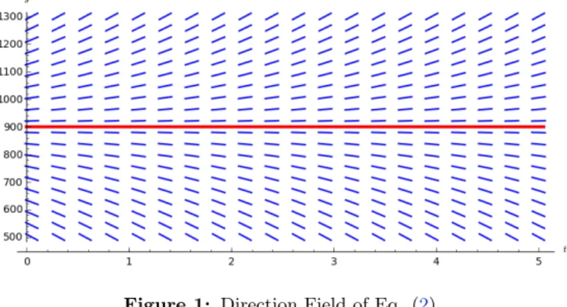
The main purpose of the course will be to learn tools to solve DE like in Eq. (2). However, behavior of the solution of Eq. (2) can be investigated without solving the diﬀerential equations. Evaluating the r.h.s. we can obtain the corresponding value of dp/dtfor diﬀerent values oftand p. For instance, whenp= 600 thendp/dt=−150 for any value of t. Similarly, dp/dt = 150 when p = 1200 independently of t. Continuing this process we obtain Figure1. This is such graphic representation of Eq. (2) is called adirection field orslope field.

(3)

Figure 1: Direction Field of Eq. (2).

Finally, one should keep in mind the limitations of any modeling that one uses to study a phenomena. Notice that the population model eventually predicts negative numbers of mice (if p < 900) or very large numbers (if p > 900 and time is large enough). This suggest that this models is unrealistic after fairly short time interval.

Example 2 (Problem 1.21). A pond initially contains 1,000,000 gal of water and an unknown amount of an undesirable chemical. Water containing 0.01 g of this chemical per gallon flows into the pound at a rate of 300 gal/h. The mixture flows out at the same rate, so the amount of water in the pond remains constant. Assume that the chemical is uniformly distributed throughout the pond.

a) Write a DE for the amount of chemical in the pound at any time.

b) How much of the chemical will be in the pond after a very long time? Does this limiting amount depend on the amount that was presently initially?

Solution:

a) Let q(t) = the amount of chemical present in the pound at time t. Assume q(t) is measured in grams and the time tin hours. The rate at which the chemical is entering the pond is

300 gallons/hour×0.01 grams/gallon.

The rate at which the chemical is leaving the pond is

300 gallons/hour×q(t)/1,000,000 grams/gallon.

Notice that since the rate at which the water is entering the pound is the same as the rate at which the water is leaving the pond, then, the amount of water in the pond is always constant. Hence is must be equal toq(0) = 1,000,000 gallons. Finally the rate of change of the chemical in the pound is

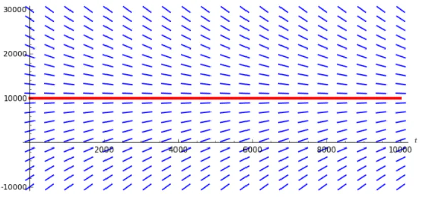
dq

dt = 3−0.0003q (3)

(4)

Figure 2: Direction Field of Eq. (3).

(5)

2 First Order Diﬀerential Equations

In this chapter we will consider DE of firs order

dy

dx =f(x, y) (4)

2.1 Separable Equations

We first consider the case when the functionf(x, y) in Eq (4) is of separable variables, that is

dy dx =

M(x)

N(y), N(y)̸= 0. (5)

In this case we obtain that the general solution is given by

∫

M(x)dx=

∫

N(y)dy+C, C∈R

2.2 Linear Equations

Consider the DE

dy

dt +p(t)y=g(t) (6)

were pand g are functions oft. If we multiply both sides by the integral factor

µ(t) =e∫p(t)dt, (7)

then the DE (6) becomes

d

dt(µ(t)y(t)) =µ(t)g(t).

Integrating both sides we obtain the general solution of DE (6)

y(y) = 1 µ(t)

(∫

µ(t)g(t)dt+C

)

, C∈R. (8)

We can also write Eq. (8) to take into account an initial condition at time t = t0, in such case we obtain,

y(t) = 1 µ(t)

(∫ t

t0

µ(s)g(s)ds+µ(t0)y(t0)

)

(9)

2.3 Modeling with First Order Diﬀerential Equations

(6)

Compound Interest

Compound interest is interest added to the principal of a deposit or loan so that the added interest also earns interest from then on. If we assume that interests are added continuously then the rate of change of the value of the deposit or loan is given by the interests times proportional to itself. Let

• S(t) the value of the deposit or loan aftert years,

• S0 the value of the principal (i.e., S(0)),

• r the annual rate of interests. Then S(t) satisfies the following DE,

dS(t)

dt =rS(t), S(0) =S0. Solving this DE by separation of variables we obtain

S(t) =S0ert. (10)

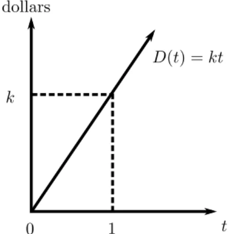
If we assume that annual deposits (or withdraws) of k dollars are made continuously and linear throughout the year. That is the total deposit function in terms of time is given byD(t) =kt.

0 1 t

D(t) =kt dollars

k

Figure 3: Deposit functionD(t) represent the total deposits made at any timet.

Let

• kbe the annual deposit made continuously.

In this case the rate of change of the value of the deposit or loan is given by

dS(t)

dt =rS(t) +k, S(0) =S0 (11)

Again using separations of variables to solve Eq (11) we get

(7)

Newton’s Law of Cooling

Newton’s Law of cooling states that the temperature of and object changes at a rate proportional to the diﬀerence between its temperature and that of its surroundings. Denote by

• T(t) the temperature of the object at time t.

• Tm the temperature of the medium.

• kthe constant of proportionality.

Then T(t) satisfies the following DE

dT(t)

dt =k(T(t)−Tm) (13)

Uniform Mixing

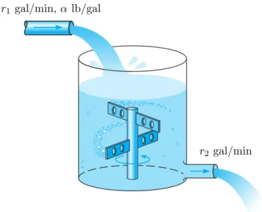
Consider a tank that contains Q0 lb of salt dissolved in V0 gal of water; see Figure 4. Assume that water containingαlb of sal/gal is entering the tank at a rate ofr1 gal/min and that well-stirred mixture is draining from the tank at a rate ofr2 gal/min.

r1 gal/min,α lb/gal

r2 gal/min

Figure 4: Mixing problem for a water tank.

Let

• Q(t) be the amount of salt at any time t.

• Q0 initial amount of salt.

(8)

• V0 initial amount of water.

• α concentration of salt of incoming water.

• r1 incoming rate of water.

• r2 outgoing rate of water.

Notice that

V(t) =V0+ (r1−r2)t

and then the concentration of salt at any time is

Q(t) V(t) =

Q(t) V0+ (r1−r2)t.

Then Q(t) satisfies the linear DE

dQ(t)

dt =r1α−

r2

V0+ (r1−r2)tQ(t), Q(0) =Q0 (14)

Remark 1. Notice that we could have incoming or outgoing rates depending on time, i.e., we can have r1(t) and/or r2(t).

Remark 2 (Other Applications of Tank Model). This tank model could be used for diﬀerent applications like, pollutant in a lake, drug in an organ of the body, etc. In such cases the flows rates may not be easy to determine or may vary with time. Similarly, the concentration may be far from uniform in some cases.

Chemical Reactions

The Law of Action of Mass states that if the temperature remains constant, the rate of the chemical reaction is proportional to the product of the concentrations of the substances that are reacting. A second order chemical reaction involved the interaction (collision) ofnmolecules of a substance P with one (1−n) molecules of a substanceQ to produce a new substanceX. Let

• x(t) be the concentration of X at timet

• pinitial concentration of P

• q initial concentration ofQ

• kthe constant of proportionality

thenx(t) solves the DE

dx(t)

(9)

Newton’s Laws of Movement

The second Newton’s law of movement says that the net vector force Fof an object is equals to the massm of that object multiplied by the vector accelerationa, i.e.,

F=m·a (16)

We limit our study when the movement is along a one-dimensional line. In such case the force F is positive if acts in the direction of the movement and negative if acts in the opposite direction.

Example 3 (Falling Object). Suppose and object of massmis falling in the atmosphere near sea level. Assume there there is drag force (due to air resistance acting upon the object) proportional to its velocity.

(a) If v(t) is the velocity of the object at time t. Write a DE for v(t) that describes the dynamics of the falling object.

(b) If the initial velocity of the object isv0 find v(t) at any timet.

(c) Find the limiting velocity of the object after a long period. This limiting velocity is called terminal velocity

Solution. (a) The forces acting upon the object are the gravitational force and the drag force. The gravitational force acts in the direction of the movement with magnitude mg, whereg≈9.8m/s2 near sea level. The drag force acts in opposite direction to the movement with magnitude equal toγv, whereγ is a positive constant of proportionality. In summary,

F=mg−γv

Hence, from Newton’s second law of movement we obtain that

mdv

dt =mg−γv, γ >0. (17)

(b) Using separation of variables to solve DE (17) and the initial condition v(0) = v0 we obtain

v(t) = mg γ +

(

v0+ mg γ

)

e−γt/m (18)

(c) Using solution (18) we get that as t → ∞, v(t) → (mg)/γ. Hence the terminal velocity is

mg γ

(10)

Notice that the distance depends on the position of the object at timet. For convenience we will write the position of the object as

R+x(t) = position at timet

whereRis a the constant radius of the earth where the experiment is taking place, and

x(t) = the distance of the object from the surface of the earth.

Using this notation we get that

d=|R+x(t)|.

In summary, the magnitude of the gravitational force is given by

k

|R+x(t)|2, k >0. (19)

Example 4 (Escape Velocity). A body of constant mass m is projected away from the earth in a direction perpendicular to the earth’s surface with and initial velocity v0. Assuming that there is no air resistance, but taking into account the variation of the earth’s gravitational field with distance.

(a) Find an expression for the velocity during the ensuing motion.

(b) Find the initial velocity that is required to lift the body to a given maximum altitude ξ above the surface of the earth.

(c) Find the least initial velocity for which the body will not return to the earth; this is called theescape velocity.

Solution. (a) The gravitational force is given by

F(x) =− k

|x+R|2, k >0.

since when x= 0 (i.e., near sea level)F=−mg withg≈9.8m/s2 the,

F(x) =− mgR 2

|x+R|2, k >0.

Since there are no other forces acting in the body, the DE of motion is given by

mdv dt =−

mgR2

|x+R|2, k >0.

Notice that the previous DE depends on three variables, namelyv, x andt. To remedy this situation we eliminate the variabletfrom the DE using the chain rule. Notice that by the chain rule

dv dt =

dv dx

dx dt =v

(11)

Hence the DE of motion becomes

vdv dx =−

gR2

(R+x)2, v(0) =v0. (20)

Notice that the initial positionx(0) = 0, hencev(0) =v0. Using separation of variables to solve DE (20) we obtain

v(x) =±

√

v₀2−2gR+ 2gR 2

R+x. (21)

Notice that Eq. (21) gives the velocity in terms of the position rather than a function of time. The plus sign must be chosen if the body is rising, and the minus sign must be chosen if it is falling back to the earth.

Exercise 1. A box of weightW lb slides downward from rest along a tilted plane. The plane makes angle with the horizontal of θ degrees. Assume the gravitational force is constant equal to 9.8m/s2_.

(a) Find the DE that for the velocityv(t) of the box at any timet.

(b) Find the acceleration, velocity and position of the box.

Population Dynamics

We consider the problem of modeling the growth or decline of the population of a given organism, an important issue in fields ranging from medicine to ecology to global economics. We first begin with a simple model and subsequently add more complexity to the analysis. In the remain of this subsection lety(t) be the population of the organism at any timet.

Exponential Growth. The simplest hypothesis concerning the variation of the population is to assume

dy

dt =ry, y(0) =y0, (22)

wereris called therate of growth or decline. Using separation of variables we know that

y(t) =y0ert (23)

Under ideal condition, Eq. (23) has been observed to be reasonably accurate for many population, at least for a small period of time. However limitation on space, food, competition will reduce the growth rate and bring and end to the exponential growth.

Logistic Growth. To take into account the fact that the growth rate depends on the population, we replace the constantr in Eq.(22) for the functionh(y) =r(1−y/K) for r >0, i.e.,

dy dt =r

(

1− y K

)

(12)

Notice thath(y) isr when y= 0 and asy increasesh(y) decreases until it reaches zero when y=K. This DE is called logistic equation. The constant r is called intrinsic growth rate andK is theenvironmental carrying capacity orsaturation level. The rate of change function f(y) = r(1−_Ky)y will be positive for 0 < y < K and negative after y > K. The point (K/2, rK/4) represents a change in the concavity of the solutions as shown in Fig. 5

Figure 5: Graph of rate change functionf(y) =r(1−_Ky)y.

We can solve this DE using separation of variables and partial fraction integration to obtain,

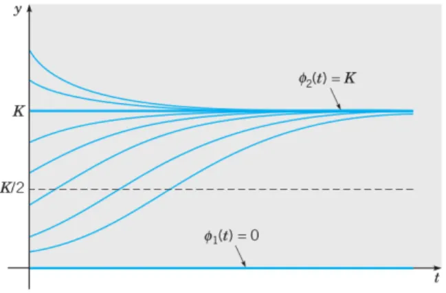
y(t) = y0K y0+ (K−y0)e−rt

(25)

The behavior of the solutions will depend on the initial conditiony0 as illustrated in Fig.

6. However, no matter the initial conditiony0 the solution approaches it environmental

Figure 6: Graph of some solutionϕ(t) is Eq. 24

carrying capacity valueK, i.e.,

lim

t→∞y(t) =K

(13)

environmental carrying capacity. However there are certain population that would need to go beyond a certain threshold parameterT to be able to remain alive. To study this type of population we introducelogistic equation with threshold

dy dt =−

(

1− y T

) (

1− y K

)

y, y(0) =y0 (26)

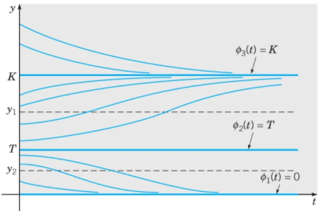
By looking at the graph of the rate of change function f(y) = −(1− _Ty) (1−_Ky)y in Fig. 7, notice that the rate of change in the population will be negative for small values

Figure 7: Graph of rate functionf(y) for the logistic equation with threshold.

ofy, 0< y < T then it will become positive until a saturation levelK and it will become negative again for y > K. Hence the solution will get to the environmental carrying capacity value K, only if y0> T. When y0 < T the population will become extinct.

The solution of Eq. 26 can only be given implicitly by

(

y(t)−K y(t) ·

y0 y0−K

)T ( _y(t)

y(t)−T · y0−T

y0

)K

=er(K−T)t (27)

However, we can use the qualitative information encoded in the graph of the rate change function to determine that graph the solution of Eq. (26).

Figure 8: Graph of solutions of the logistic equation with threshold.

(14)