THE STATISTICAL ANALYSIS OF GENETIC SEQUENCING AND RARE VARIANT ASSOCIATION STUDIES
Eugene Urrutia
A dissertation submitted to the faculty at the University of North Carolina at Chapel Hill in partial fulfillment of the requirements for the degree of Doctor of Philosophy in
the Department of Biostatistics in the Gillings School of Global Public Health.
Chapel Hill 2013
c
2013
ABSTRACT
Eugene Urrutia: The Statistical Analysis of Genetic Sequencing and Rare Variant Association Studies
(Under the direction of Michael Wu)
Understanding the role of genetic variability in complex traits is a central goal of modern human genetics research. So far, genome wide association tests have not been able to discover SNPs that explain a large proportion of the heritability of disease. It is hoped that with the advent of accessible DNA sequencing data, investigators can uncover more of the so-called missing heritability. The added information contained in sequencing data includes rare variants, that is, minor alleles whose population frequency is low.
We examine several existing region based rare variant association tests including burden based tests and similarity based tests and show that each is most powerful under a certain set of conditions which is unknown to the investigator. While some have proposed tests that combine the features of several existing tests, none as yet has provided a test to combine the features of all existing tests. Here, we propose one such test under the framework of the SKAT test, and show that it is nearly as powerful as the most appropriately chosen test under a range of scenarios.
TABLE OF CONTENTS
LIST OF TABLES . . . ix
LIST OF FIGURES. . . xii
1 Introduction and Overview . . . 1
2 Literature Review . . . 4
2.1 Statistical methods of testing whole genetic sequencing regions . . . 4
2.1.1 Heritability of disease . . . 4
2.1.2 Statistical methods of testing genome-wide association studies . . . 5
2.1.3 Burden based sequence association tests . . . 6
2.1.4 Similarity based sequence association tests . . . 7
2.1.5 Sequence Kernel Assocation Test . . . 8
2.1.6 Combination based sequence association tests . . . 12
2.2 Statistical methods for working with missing covariates . . . 14
2.2.1 Mechanisms of missingness . . . 14
2.2.2 Complete case . . . 16
2.2.3 Single and multiple imputation . . . 16
2.2.4 Maximum likelihood . . . 18
2.2.5 Weighted maximum likelihood for data with missing covariates . . . 19
2.3 Statistical methods of selecting rare genetic variants within a genetic region . . . 21
2.3.1 Variable Selection . . . 21
2.3.3 Multivariable linear model . . . 22
2.3.4 Penalized linear regressions . . . 23
2.3.5 Consistent LASSO-based procedures . . . 24
2.3.6 Stability Selection . . . 25
3 Rare Variant Testing Across Methods and Thresholds Using the Multi-Kernel Sequence Kernel Association Test (MK-SKAT) . . . 27
3.1 Introduction . . . 27
3.2 Methods . . . 29
3.2.1 Connections between SKAT and other Methods . . . 30
3.2.2 Multi-Kernel Sequence Kernel Association Test . . . 34
3.2.3 Simulations . . . 36
3.3 Results . . . 39
3.3.1 Type I Error and Power . . . 39
3.3.2 Data Analysis . . . 42
3.4 Discussion . . . 43
4 Accommodating Partially Missing Covariates in the Sequence Kernel Association Test for Rare Variants . . . 46
4.1 Introduction . . . 46
4.2 Methods . . . 49
4.2.1 SKAT . . . 49
4.2.2 Regression with Partially Missing Covariates . . . 50
4.2.3 Accommodating Missing Covariate Information in Tests of Rare Variants . . . 55
4.2.4 Continuous Missing Covariates and Multiple Missing Covariates . . . 57
4.3 Results . . . 59
4.3.2 Power Simulations . . . 60
4.4 Discussion . . . 62
5 Kernel Machine Testing using Maximum Likelihood by IRLS for Gene Level Analysis of Methylation Data with Missing Covariates . . . 64
5.1 Introduction . . . 64
5.2 Simulations . . . 66
5.2.1 Type I Error . . . 67
5.2.2 Power Simulations . . . 68
5.3 Application to Epigenetic Study of Birth Weight . . . 71
5.4 Discussion . . . 73
6 Evaluation of Statistical Methods for Prioritization and Selection of Individual Rare Variants in Sequence Association Studies . . . 76
6.1 Introduction . . . 76
6.2 Methods . . . 79
6.2.1 Marginal Analysis . . . 80
6.2.2 Lasso Based Methods . . . 81
6.2.3 Stability Selection . . . 82
6.2.4 Forward Selection . . . 83
6.3 Simulations . . . 83
6.3.1 Evaluative Metrics . . . 85
6.3.2 Results . . . 86
6.4 Data Analysis . . . 87
6.4.1 Overview . . . 87
6.4.2 Results . . . 90
6.5 Discussion . . . 90
A2 Derivation of IRLS Newton Raphson: Partially Observed
Continuous Covariate . . . 93
LIST OF TABLES
2.1 Summary of commonly used statistical methods of
testing whole genetic sequencing regions . . . 14
2.2 Summary of methods to account for missing covariates. Imupation valid under MAR only when full likelihood
posterior distribution used to fill-in missing data. . . 21
2.3 Summary of methods of variable selection . . . 26
3.1 Type I error simulation results for quantitative traits. Each cell in the table corresponds to the type I error of SKAT using a kernel constructed based on the testing procedure at the top of the table and the grouping strategy at the left of the table. Rows and columns labeled MK-SKAT correspond to the omnibus tests across tests (with fixed group) and across groupings (with fixed test). The cells with both rows and columns labeled MK-SKAT correspond
to the omnibus test across all test and groupings. . . 39
3.2 Type I error simulation results for dichotomous traits. Each cell in the table corresponds to the type I error of SKAT using a kernel constructed based on the testing procedure at the top of the table and the grouping strategy at the left of the table. Rows and columns labeled MK-SKAT correspond to the omnibus tests across tests (with fixed group) and across groupings (with fixed test). The cells with both rows and columns labeled MK-SKAT correspond
to the omnibus test across all test and groupings. . . 40
3.3 Power results for Setting 1. Each cell in the table corresponds to the power of SKAT using a kernel constructed based on the testing procedure at the top of the table and the grouping strategy at the left of the table. Rows and columns labeled MK-SKAT correspond to the omnibus tests across tests (with fixed group) and across groupings (with fixed test). The cells with both rows and columns labeled MK-SKAT correspond to the omnibus test across all
3.4 Power results for Setting 2. Each cell in the table corresponds to the power of SKAT using a kernel constructed based on the testing procedure at the top of the table and the grouping strategy at the left of the table. Rows and columns labeled MK-SKAT correspond to the omnibus tests across tests (with fixed group) and across groupings (with fixed test). The cells with both rows and columns labeled MK-SKAT correspond to the omnibus test across all
test and groupings. . . 41
3.5 Power results for Setting 3. Each cell in the table corresponds to the power of SKAT using a kernel constructed based on the testing procedure at the top of the table and the grouping strategy at the left of the table. Rows and columns labeled MK-SKAT correspond to the omnibus tests across tests (with fixed group) and across groupings (with fixed test). The cells with both rows and columns labeled MK-SKAT correspond to the omnibus test across all
test and groupings. . . 42
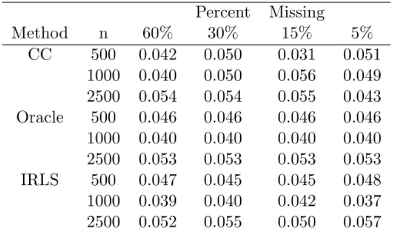
4.1 Type I error simulation results at the α = 0.05 level comparing SKAT using complete case (CC), SKAT with IRLS to accommodating missing values (IRLS), or SKAT assuming that the missing values
are known (Oracle). . . 60
5.1 Estimates of type I error in the application of kernel machine testing with complete case (cc) treatment of missing data, with oracle knowledge of the missing covariate values, and with ML by IRLS based analysis. Estimates are based on 10,000 simulated null model data sets under different sample sizes (n), signifiance levels (α), and percentage missingness (%mis). CpGs
are uncorrelated here. . . 69
5.2 Estimates of covariate effects on birth weight. The two procedures used are complete case and maximum
likelihood by iteratively reweighted least squares . . . 74
5.3 Raw and Bonferroni Corrected p-values for the top results from the real data analysis. Kernel machine testing with maximum likelihood via IRLS is denoted by IRLS. Complete case analysis with kernel machine
6.1 Comparison of methods in ability to correctly identify causal variants for default simulation setting. Measures of comparison include true positives, false positives, and true postitives indexed by minor allele frequency. Additionally presented is a rankscore, which measures ability to informatively order variants by level of importace, with 1 meaning all 20 top ranked variants
are causal, and 0 meaning none are causal. . . 87
6.2 Real data application: Comparison of methods in number of variants identified as being associated with homeostatic model assessment levels. Measures of comparison include total selected variants, and selected
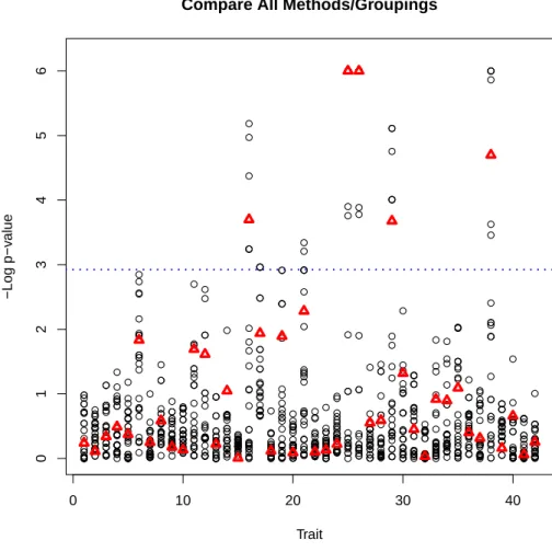
LIST OF FIGURES 3.1 Real data analysis results. Each column of circles
corresponds to the p-values from analyzing a different trait while each circle represents the p-value from a different kernel. The triangle indicates the p-value from applying MK-SKAT to all of the kernels. p-values have been truncated at 10−6. The blue line
indicates the bonferroni significance level. . . 44
4.1 Data augmentation using the approach of Ibrahim
(1990) involves expanding each observation with missingness based on values that the missing variable can take.
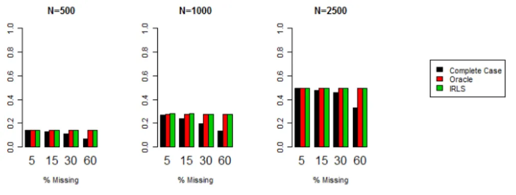
Here we assume that X2 is dichotomous. . . 53 4.2 Power simulation results comparing SKAT using complete
case (CC), SKAT with IRLS to accommodating missing values (IRLS), or SKAT assuming that the missing
values are known (Oracle). . . 61
5.1 Scaled estimates of type I error in the application of kernel machine testing with complete case (cc) treatment of missing data, with oracle knowledge of the missing covariate values, and with ML by IRLS based analysis. Horizontal line indexes the ideal type I error level (alpha) and scaled to 100. Estimates are based on 10,000 simulated null model data sets under different signifiance levels, percentage missingness, and correlation structures. Sample size is fixed at
n= 500. . . 70 5.2 Scaled power estimates for kernel machine testing
with complete case (cc) treatment of missing data, with oracle knowledge of the missing covariate values, and with ML by IRLS based analysis. Estimates are based on 10,000 simulated null model data sets under different signifiance levels, percentage missingness, and correlation structures. The effect size depended on the correlation structure to avoid saturation. Sample
6.1 Simulation results for varied sample size. Left column compares methods by true postives and false postives, with total observed causal variants and total variants noted for comparison. Middle column compares methods by true postives with respect to minor allele frequency, with total observed variant by MAF noted for comparison. Right column compares methods by their ability to order variants by rank of importance, with 0 worst
and 1 perfect. . . 88 6.2 Simulation results for varied prior information. Left
column compares methods by true postives and false postives, with total observed causal variants and total variants noted for comparison. Middle column compares methods by true postives with respect to minor allele frequency, with total observed variant by MAF noted for comparison. Right column compares methods by their ability to order variants by rank of importance,
Chapter 1
Introduction and Overview
In modern human genetics, it is desired to know whether genetics play a role in phenotype, for example the presence or absence of a disease. So far, genome wide association tests have not been able to discover SNPs that explain a large proportion of the heritability of disease. It is hoped that with the advent of accessible DNA sequencing data, investigators can uncover more of the so-called missing heritability. The added information contained in sequencing data includes rare variants, that is, minor alleles whose population frequency is low. This is in contrast to microarray technology which typically includes common single nucleotide polymorphisms whose minor allele frequency (MAF) are relatively high. Rare variants associated with disease have already been reported.
Statistical considerations need to be made to adjust to rare variant association testing. Power decreases substantially when applying common variant methodology to rare variants. The signal is lower due to fewer minor alleles present in a given study. Also, multiple comparison corrections are a concern since the number of variants is increased dramatically.
unknown to the investigator. While some have proposed tests that combine the features of several existing tests, none as yet has provided a test to combine the features of all existing tests. Here, we propose one such test under the framework of the SKAT test, and show that it is nearly as powerful as the most appropriately chosen test under a range of scenarios.
It is of prime importance for investigators to consider important covariate information when performing genetic sequencing studies. If individual characteristics such as demographics, age, gender, or lifestyle, is ignored, many false positive results may be discovered which will not hold up under subsequent study. Fortunately, most of the widely used statistical procedures for rare variants are able to accommodate covariates. Methods have been developed to account for missing genotype via imputation or allele dosages. However, existing methods do not allow for missing covariates. In the case of missing covariates, misleading results may be obtained if proper adjustments are not provided. For example, if the data are missing at random, and only complete observations are used in the analysis, then there is a great danger of biased parameter estimation. In paper 2, we examine the properties of complete case, single/multiple imputation, and maximum likelihood when covariates are MCAR and MAR. We use an existing maximum likelihood strategy via iteratively reweighted least squares and apply it to the SKAT framework for rare variant association testing. This results in a test that maximizes power while still providing unbiased estimation and correct control of type I error under the condition of missing covariates under MAR.
simulated data and real data. Furthermore, we consider the direct use of forward selection in conjunction with SKAT and show that this method is highly competitive and can often select truly causal variants.
In the review of the current literature, we describe the following: 1. Statistical methods of testing whole genetic sequencing regions
2. Statistical methods for working with missing covariates
3. Statistical methods of selecting rare genetic variants within a specific genetic region
We follow with our own contributions to rare variant association testing:
1. Multiple kernel SKAT unified framework for rare variant association testing
2. Maximum likelihood based procedure for rare variant sequencing data with missing covariates
Chapter 2
Literature Review
2.1 Statistical methods of testing whole genetic sequencing regions
2.1.1 Heritability of disease
In genetic association testing, it is desired to know whether genetics play a role in phenotype, for example the presence or absence of a disease. Heritability, the inheritance of phenotypes such as disease resulting from genetic information alone, can be estimated using family based studies (McNeill et al., 2004; Dwyer et al., 1999). For example, identical twins separated at birth have identical genetic information and randomly associated environmental factors, while random pairs of persons have random genetic similarity and randomly associated environmental factors. Linear mixed modeling of an outcome can estimate the variance due to heretability versus that due to environment.
missing heritability: the technological advance of whole genome DNA sequencing.
The added information contained in DNA sequencing data includes rare variants, that is, minor alleles whose population frequency is low, well below the 5% threshold of common variants used in microarray studies. Already, rare variants associated with disease have been reported (Cohen et al., 2006; Walsh et al., 2008; Nejentsev et al., 2009).
We begin by briefly discussing the methods previously used in GWAS and then discuss the adaptations used in sequencing association studies.
2.1.2 Statistical methods of testing genome-wide association studies
The most popular statistical method of GWAS is regression applied to case-control or quantitative trait data (Hunter et al., 2007; Yeager et al., 2007; Thomas et al., 2008; Scott et al., 2007). Demographics such as gender, race, and age are controlled for and p-values are adjusted for multiple comparisons. Chi-squared test stratified for discrete covariates can be used but is impractical for covariates in comparison to logistic regression. For continuous phenotypes such as blood pressure, linear regression with the identity link is used similarly to logistic regression.
2.1.3 Burden based sequence association tests
One class of region based methods is the burden-based class of tests. In the cohort allelic sum test and combined multivariate collapsing test (CAST/CMC) the genetic information of a region for an individual is collapsed to a single binary variable which takes the value 1 if the person has at least one rare variant present in the region and 0 otherwise (Morgenthaler and Thilly, 2007; Li and Leal, 2008). In a slight variation, the count collapsing method, the summary variable takes the value of the total number of rare variants present in the region of an individual (Morris and Zeggini, 2010). Additionally, one may wish to place a higher weight on variants which are rarer, and this is done in the weighted count collapsing method (Madsen and Browning, 2009). The burden-based rare variant association tests are similar in that they sum over the rare variant genetic information. Thus, they are most powerful when the effects of the variants are all in the same direction, that is, all are deleterious or all are protective. Power is decreased when effects are in opposite directions.
Assuming continuous outcome (yi) , the above models are described below and solved
using linear regression: CAST/CMC:
yi=αXi+βI( p X
j=1
zij >0) +i
Count Collapsing:
yi=αXi+β p X
j=1
zij+i
Weighted Count Collapsing:
yi=αXi+β p X
j=1
zijwj+i
whereXi are covariates including intercept; zij is the number of rare alleles present at locus
j in individual i and takes the value 0, 1, or 2; andwj is an assigned weight, typically higher
for the rarer variables.
(KBAC) to address statistical problems associated with misclassification of variant functionality, causality, and polymorphism status, and also with gene interactions. Using the cumulative minor-allele test (CMAT), Zawistowski et al. (2010) have broadened the scope to the application of low-coverage sequencing and imputation data, as well as population stratification. Bhatia (2009) proposed RARECOVER in order to take advantage of a subset within a region being more associated with a phenotype. Still, though, none of the methods mentioned yet address the concern of variants within a region having both deleterious and protective effects.
Investigators have developed and adapted new strategies to address this concern. Han and Pan (2010a) introduced the data-adapted sum (aSum) test which incorporates both marginal (univariable) analysis and common association strength to detect both protective and deleterious effects. Ionita-Laza et al. (2011) introduced another novel strategy, the replication-based strategy, to achieve the same. Li et al. (2010a), with their weighted haplotype and imputation-based tests (WHaIT), added imputation capabilities to the protective/deleterious model.
2.1.4 Similarity based sequence association tests
Others have proposed another set of tests called similarity-based methods. In this class the question is asked whether individuals who are genetically similar are also phenotypically similar. Neale et al. (2011) adapted the C-alpha score test to evaluate change in variance of the allele frequency rather than change in the mean of the allele frequency in cases compared to controls. Under the null hypothesis of no genetic association with outcome, distribution of counts of rare alleles should follow the binomial distribution. By testing variance rather than net effect, the test is powerful to detect genetic association when the effects of the variants are not all in the same direction.
and null hypothesis of equal distribution among cases and controls:
T = √1
c
m X
j=1
(zj−njp0)2−njp0(1−p0)
wherezj is the total rare allele count for variantjin cases only,nj is the total rare allele count
for variant j in both cases and controls, p0 is the proportion of cases out of total subjects,
and c is a standardization term.
2.1.5 Sequence Kernel Assocation Test
Another similarity-based method, the sequence kernel association test (SKAT), includes the flexibility to custom define what is genetic similarity through a kernel function (Wu et al., 2011). The result is an n by n matrix of pair wise genetic similarity which appears very much like a correlation matrix. SKAT is our preferred method because it offers a general framework that is adaptable to almost any scenario while retaining power when the kernel is chosen appropriately. It is also flexible in that covariates can be accomodated without the use of permutation.
SKAT is based on a semi-parametric model:
yi=xiβ+h(zi) +i
h(.) is defined by the kernel function K(., .). In general two popular kernel functions are the dth polynomial kernel and the gaussian kernel.
Dth polynomial kernel:
K(z1, z2) = (z1Tz2+ρ)d
where d indexes the order of polynomial andρ is an index parameter
When d = 1, this is equivalent to a linear function space with first-order basis functions:
{z1, z2, . . . , zm}. When d = 2, this is equivalent to a quadratic function space with
Gaussian kernel:
K(z1, z2) = exp{−||z1−z2||2/ρ}
whereρ is the scale parameter.
The Gaussian kernel is equivalent to the radial basis functions.
The kernel for the default SKAT test uses weights equal to the β(1,25) distribution evaluated at the study-wide frequency of the particular minor allele. This produces greater power when the rarest alleles have the most effect on the outcome:
Default SKAT kernel:
K=ZW(ZW)T
where Z is the full genetic design matrix and W is a diagonal matrix of weights Expanded, the default SKAT kernel takes the form:
KSKAT =
w1z11 w2z12 . . . wmz1m
w1z21 w2z22 . . . wmz2m
..
. ... ... ...
w1zn1 w2zn2 . . . wmznm
w1z11 w2z12 . . . wmz1m
w1z21 w2z22 . . . wmz2m
..
. ... ... ...
w1zn1 w2zn2 . . . wmznm T
Thus,K(z1, z2) = Pmj=1wj2z1jz2j. It is clear that K(z1, z2) approaches 1 when there is high
genetic similarity, approaches -1 when there is great genetic dissimilarity, and is close to 0 otherwise. This similarity is weighted toward rare variants.
There are several ways to estimate the parametersβandh. LSKM estimates by minimizing a scaled penalized likelihood function.
LSKM minimizes:
J(h, β) =−1
2
n X
i=1
{yi−xTi β−h(zi)}2−
1 2λ||h||
2
function can be written:
J(α, β) =−1
2
n X
i=1
{yi−xTiβ−
n X
j=1
αiK(zi, zj)}2−
1 2λα
TKα
with solutions
ˆ
β={XT(I+λ−1K)−1X}−1XT(I+λ−1K)−1y
ˆ
α=λ−1(I+λ−1K)(y−Xβˆ)
However, Liu et al. (2007a) argue that the usefulness of the LSKM is limited due to the high computing cost of estimating λ and lack of literature on estimating ρ and σ2. Thus, it is
preferable to use the linear mixed model. Linear mixed model:
y=xβ+h+
whereh are random effects with distribution N(0, τ K) and are residuals with distribution
N(0, σ2I). It is clear that this model is equivalent to LSKM becauseβ and hcan be derived equivalent to those from LSKM using a standard linear mixed model estimating procedure:
XTR−1X XTR−1
R−1X R−1+ (τ K)−1
β
h
=
XTR−1y
R−1y
whereR=σ2I and τ =λ−1σ2
When we apply the kernel machine to genetic sequencing data, we are primarily interested in whether or not the entire genetic region has an effect on the outcome. This test is:
H0 :h(z) = 0 vs. Ha :h(z)6= 0. Using the linear model framework, we can equivalently test
H0 : τ = 0 vs. Ha : τ > 0. The test falls on the boundary. Also, because K is not block
diagonal,τ is not distributed as a mixture ofχ20 and χ21.
SKAT score test statistic:
Qτ( ˆβ, σ2, ρ)−tr{P0K(ρ)}
where
Qτ( ˆβ, σ2, ρ) =
(y−xβˆ)TK(y−xβˆ) 2ˆσ2
and
P0=I −X(XTX)−1X
where ˆβ and ˆσ are estimated under the standard linear model with covariates only.
Under the null hypothesis, the quantity (y−xβˆ) converges to a standard normal, thus Q, quadratic in (y−xβˆ), is distributed κχν2, a scaled mixture of χ2, and κ and ν are calculated using one of several methods. We typically use the moment matching method described by Liu et al. (2009), although other chi-square approximation methods are available (Satterthwaite, 1946; Davies, 1980; Duchesne and Lafaye De Micheaux, 2010).
Satterthwaite approximates the null distribution with the following:
κ= ˜Iτ τ/2˜
˜
ν = 2˜2/I˜τ τ
where
˜
Iτ τ =Iτ τ−Iτ σ2I−1 σ2σ2I
T τ σ2
Iτ τ =tr{P0K(ρ)}2/2
Iτ σ2 =tr{P0K(ρ)P0}/2
Iσ2σ2 =tr{P02}/2
˜
=tr{P0K(ρ)}/2
To generate the p-value, Q is compared the null distribution of
P01/2KP01/2
2
When the outcome is continuous:
P0=I−X˜( ˜XTX˜)−1X˜T
When the outcome is case/control:
P0=D0−D0X˜( ˜XTD0X˜)−1X˜TD0
Where X is a matrix of covariates including intercept; andD0is a diagonal matrix of ˆpj(1−pˆj),
where ˆpj is the predicted proportion of rare alleles for variantjand is estimated from logistic
regression of X on Y.
2.1.6 Combination based sequence association tests
We have thus far described 5 tests used for rare variant association testing, and there are numerously many more to choose from as well. The investigator must choose one from these many options before testing the data. A second choice that the investigator must make is what will be defined as a rare variant. Choices of rare variants thresholds include variants 3% MAF, 1% MAF, or 0.5% MAF. Additionally, the investigator may want to restrict to a set of only non-synonymous mutations, or those that are biologically predicted to be ”harmful” by Polyphen-2 or other software. The result is that the investigator has many tests to choose from and many groupings to choose from as well, creating a very large set of combinations.
type I error.
A final class of gene sequence association tests attemps to solve the problem by combining several tests at once in order to have power in a range of scenarios. The variable threshold test (Price et al., 2010), for example, starts with a foundation of the score test based on the likelihood function. However, instead of picking a fixed threshold of say 3% minor allele frequency, they select a range of different minor allele frequency thresholds. The score test is computed at each threshold, and a final p-value is found through permutation, so that type I error is conserved.
Optimal tests for rare variant effects in sequencing association studies (SKAT-O) (Lee et al., 2012), on the other hand, tests over a range of tests that spans from the count test to the SKAT test. That is, it tests on one hand that effect sizes and directions of the various rare alleles are perfectly corrlelated, and also the other hand that there is no correlation in effect sizes. Scenarios in between are tested as well. Thus, whileKSKAT may be written:
KSKAT =ZwZwT
SKAT-O can be expanded as:
KSKAT−O=ZwRρZwT
Where Zw is the weighted minor allele frequency design matrix, and Rρ is the corellation
matrix indexed byρ where:
Rρ= (1−ρ)I+ρ11T
Lee et. al use the minimum p-value as the test statistic and the final p-value is found by integrating the distribution function of the null mixture of χ2 distribution.
An additional combination test was introduced by Lin and Tang (2011). The general framework allows not only test a range of MAF thresholds, but is also capable of handling covariates without the need for permutation.
Lin’s score statistic is:
Uk= n X
Yi−
eYˆi
1 +eYˆi
!
ξkTZiV −1/2
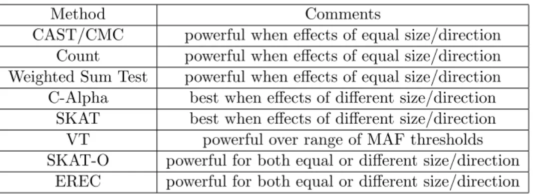
Method Comments
CAST/CMC powerful when effects of equal size/direction Count powerful when effects of equal size/direction Weighted Sum Test powerful when effects of equal size/direction C-Alpha best when effects of different size/direction
SKAT best when effects of different size/direction VT powerful over range of MAF thresholds SKAT-O powerful for both equal or different size/direction
EREC powerful for both equal or different size/direction
Table 2.1: Summary of commonly used statistical methods of testing whole genetic sequencing regions
where ˆYi is estimated under the null (covariates only),ξk is a kernel specific weight function,
and Vk is the kernel specific variance of the score statistic.
Lin shows that the for the optimal kernel choice,ξj=βj. To attempt to achieve optimality,
he introduced estimated regression coefficients (EREC). EREC:
ξj = ˆβj±δ
Whereδ is a given constant, and ˆβj is the regression coefficient estimated from the data.
ξj will converge to βj ifδ decreases to 0 as the sample size n increases to N
2.2 Statistical methods for working with missing covariates
2.2.1 Mechanisms of missingness
Covariates are important to all statistical anlaysis. They can increase power when properly used, and can lead to inflated type I error when improperly used or ignored. In this section, we discuss the methods used to address partially missing covariates.
convenient to assign the valueri to 1 if x2i is observed and to 0 if x2i is unobserved (N/A) .
Y X1 X2 R
y1 x11 x21 1
y2 x12 x22 1
y3 x13 N/A 0
y4 x14 x24 1
y5 x15 N/A 0
..
. ... ... ...
yn x1n x2n 1
There are, in general, three missing data mechanisms, that is, three underlying models which predict which data points are missing. Data missing completely at random (MCAR) is randomly missing, that is, not predictable by any observed or unobserved data points. Data missing at random (MAR) may be missing in a way predictable by observed data points, but is not predictible by unobserved data points. Data not missing at random (NMAR) may be predictable by data observed or unobserved.
To summarize with our data set, again assuming x2 but notx1 has missingness: Missing completely at random:
R⊥f(y, x1, x2)
Missing at random:
R⊥f(x2|y, x1)
Not missing at random:
R=f(x2|y, x1)
2.2.2 Complete case
Complete case is a very simple method used where all observations with at least one missing covariate are excluded from analysis. Complete case transforms the incomplete data set to a complete data set which is more convenient to work with:
Complete case:
Y X1 X2 R
y1 x11 x21 1
y2 x12 x22 1
y3 x13 N/A 0
y4 x14 x24 1
y5 x15 N/A 0
..
. ... ... ...
yn x1n x2n 1 −→
Y X1 X2
y1 x11 x21
y2 x12 x22
y4 x14 x24
..
. ... ...
yn x1n x2n
It is clear, however, that complete case will result in reduced power due to the decrease in sample size. Additionally, statistical inference on the full data using only the complete case is invalid under MAR and NMAR. Bias is likely to result (Little and Rubin, 1987; Knol et al., 2010).
2.2.3 Single and multiple imputation
Single imputation using mean to fill in missing observations:
Y X1 X2 R
y1 x11 x21 1
y2 x12 x22 1
y3 x13 N/A 0
y4 x14 x24 1
y5 x15 N/A 0
..
. ... ... ...
yn x1n x2n 1 −→
Y X1 X2
y1 x11 x21
y2 x12 x22
y3 x13 x2
y4 x14 x24
y5 x15 x2
..
. ... ...
yn x1n x2n
Multiple imputation using random values based on the empirical distribution:
Y X1 X2 R
y1 x11 x21 1
y2 x12 x22 1
y3 x13 N/A 0
y4 x14 x24 1
y5 x15 N/A 0
..
. ... ... ...
yn x1n x2n 1 −→
Y X1 X2 R
y1 x11 x21 1
y2 x12 x22 1
y3 x13 x2+ 0
y4 x14 x24 1
y5 x15 x2+ 0
..
. ... ... ...
yn x1n x2n 1
Y X1 X2 R
y1 x11 x21 1
y2 x12 x22 1
y3 x13 x2+ 0
y4 x14 x24 1
y5 x15 x2+ 0
..
. ... ... ...
yn x1n x2n 1
Where∼N(0,σˆ2x2) assuming x2 is normally distributed.
Imputation has an advantage over complete case in that data is not thrown away. This clearly will increase power simply due to increased sample size. The two examples shown are valid under MCAR (Little and Rubin, 1987). Imputation is unbiased under MAR only when full likelihood posterior distribution used to fill-in missing data.
2.2.4 Maximum likelihood
possible values of the missing covariate. Maximum likelihood:
whenx2 is observed:
p(yi, x2i, ri|x1i, β, α, ω) =p(yi|x1i, x2i, β)p(x2i|x1i, α)p(ri|yi, x1i, ω)
while for missingx2 (continuous):
p(yi, ri|x1i, β, α, ω) =p(ri|yi, x1i, ω) Z
x2i
p(yi|x1i, x2i, β)f(x2i|x1i, α)dzi
or for missingx2 (discrete):
p(yi, ri|x1i, β, α, ω) =p(ri|yi, x1i, ω) X
x2i
p(yi|x1i, x2i, β)p(x2i|x1i, α)
In summary, the log-likelihood is:
rilog [p(yi, x2i, ri|x1i, β, α, ω)] + (1−ri) log [p(yi, ri|x1i, β, α, ω)]
which can be solved throught either the Newton-Raphson method or by the Expectation-Maximization (EM) algorithm.
ML leads to unbiased results under MAR if the model is correctly specified. This is a clear advantage over complete case and over most cases of imputation. An additional advantage of ML over imputation is that ML produces the same result each time, while MI (as well as SI with errors) leads to differing results because of the variability of the imputed data.
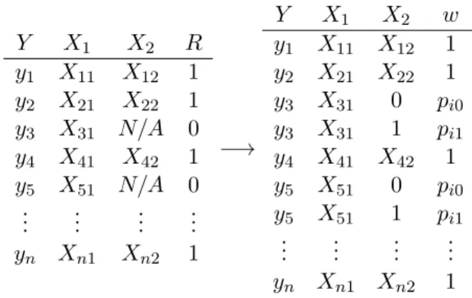
2.2.5 Weighted maximum likelihood for data with missing covariates
simple example, the covariate is dichotomous:
Y X1 X2 R
y1 x11 x21 1
y2 x12 x22 1
y3 x13 N/A 0
y4 x14 x24 1
y5 x15 N/A 0
..
. ... ... ...
yn x1n x2n 1 −→
Y X1 X2 w
y1 x11 x21 1
y2 x12 x22 1
y3 x13 0 pi0 y3 x13 1 pi1 y4 x14 x24 1 y5 x15 0 pi0 y5 x15 1 pi1
..
. ... ... ...
yn x1n x2n 1
wherepi0= 1−pi1 =P(x2= 0|yi, x1i); and generally for missing x2i:
wi =
p(yi|x1i, x2i, β)p(x2i|x1i, α) P
x2ip(yi|x1i, x2i, β)p(x2i|x1i, α)
whilewi = 1 for non-missingx2i.
Following Ibrahim, the expressions take the form of a weighted complete data log-likelihood based onN =Pni=1ki observations, whereki is the number of distinct covariate patterns for
observation i. Thus, iteratively reweighted least squares (IRLS) is used in conjunction with the Newton Raphson algorithm to solve for β and α. This Newton-Raphson algorithm is considerably more convenient when maximum likelihood cannot be solved in closed form; there is no sum or integral.
When the missing covariate is continuous, Ibrahim et al. (2004) suggest approximating
f(x2i|x1i) by a discrete distribution and then monte carlo is used to select L distinct points
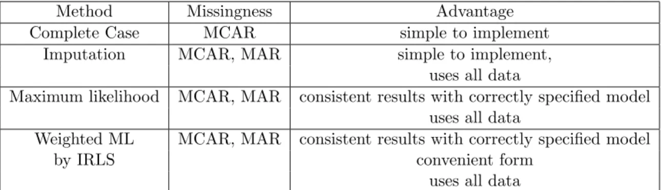
Method Missingness Advantage
Complete Case MCAR simple to implement
Imputation MCAR, MAR simple to implement, uses all data
Maximum likelihood MCAR, MAR consistent results with correctly specified model uses all data
Weighted ML MCAR, MAR consistent results with correctly specified model
by IRLS convenient form
uses all data
Table 2.2: Summary of methods to account for missing covariates. Imupation valid under MAR only when full likelihood posterior distribution used to fill-in missing data.
2.3 Statistical methods of selecting rare genetic variants within a genetic region
2.3.1 Variable Selection
Variable selection is the practice of selecting the subset of variables which best predicts the outcome. In most situations, this is beneficial to simplify a statistical model for a number of reasons. It is a simpler model to explain to others. The best and simplest model has the least variabilty in a subsequent data set. Also, during data collection, it is less costly to record fewer variables.
In our particular setting, we first discover a genomic region that is believed to be associated with the outcome by utilizing a region-based tests. It has now become necessary to find which of the specific variants within the region are the ones responsible for the association. It is the general inherent belief that some genetic variants are detrimental, some fewer are protective, and that many have absolutely no effect at all. Because of the prior belief that many variants have zero effect, we practice variable selection to find the variants that do have an effect or association and that are predictive of the outcome in a future data set. This is the second step in genetic sequence association testing.
Assuming exponential family:
g(y) =αX+βZ
zj ∈S ⇔βj 6= 0
of the outcome in a future data set. It is true that some variants not belonging to S may be associated with the outcome through colinearity with predictive variants. These variants would also be helpful in pointing us toward a true biological phenomenon.
Many variable selection procedures are particularly well suited, as they assume most of the variables have no effect and a small subset of variable may have a non-zero effect on the outcome. This leads to easier model interpretation and greater power to detect effects.
Common examples of variable selection procedures include the Lasso (Tibshirani, 1996) and forward or backward stepwise subset selection. Many other simple statistical procedures could be applied toward variable selection as well. For example, one could apply a standard procedure and apply a pre-specified cutoff for effect size or p-value.
2.3.2 Univariable linear model
The simplest variable selection procedure is the univariable model. Here each genetic variant is tested for marginal association independently of the other variants. One may use generalized linear model or generalized linear mixed model to generate a p-value associated with each variant and then apply a multiple comparison correction to generate a list of statistically significant associations.
2.3.3 Multivariable linear model
Another classic way of testing is the multivariable model where all variants are tested together in a single model and then multiple comparison correction is applied to each of the p-values. One main difference between univariate and multivariate is that the multivariate may miss some variants that are masked due to high corellation with another variant in the model. The univariate does not suffer from this problem.
2.3.4 Penalized linear regressions
A special class within the multivariable linear model are the penalized regressions. Among these, the Lasso is particularly attractive because it inherently sets the effect size of most the variables to zero, and the remaining few to non-zero. It is also computationally fast. The penalization term is customarily optimized by 10-fold cross-validation.
Lasso penalizes the sum of absolute values of regression coefficients:
n X
i=1
||g(yi)−Xiβ||2+λ
m X
j=1
||βj||1
The following are other penalized regressions, which also tend to limit the number of variables in the model:
1. Akaike information criterion (AIC) (Akaike, 1974), and Bayesian information criterion (BIC) (Schwarz, 1978) penalize the number of parameters in the model, thus clearly performs variable selection:
n X
i=1
||g(yi)−Xiβ||2+λ
m X
j=1
||βj||0
whereλis a constant for AIC, andλis proportional to the sample size for BIC.
2. Ridge regression (Hoerl and Kennard, 1970) penalizes the sum of squares of regression coefficients and thus scales parameters instead of scaling to zero.
n X
i=1
||g(yi)−Xiβ||2+λ
m X
j=1
||βj||2
3. Elastic Net (Zou and Hastie, 2005), a combination of ridge and lasso, penalizes both the the absolute value and square of regression coefficients, thus can perform both selection and scaling depending on weight ofλ1 and λ2:
n X
i=1
||g(yi)−Xiβ||2+λ1
m X
j=1
||βj||2+λ2
m X
j=1
2.3.5 Consistent LASSO-based procedures
Fan and Li (2001) contend that a good penalty function should should produce an estimator with the following properties : Unbiasedness, sparsity, and continuity. The Lasso estimates are sparse and continuous, and Lasso is in fact the only sparse and continuous penalty within the family of λ|β|q, for some q. That is, q=1 is the only q which produces
sparse and continuous estimates. AIC and BIC achieve sparsity but are not continuous inβ. Ridge regression is continuous but do not achieve sparsity. However, Lasso is not unbiased, as large coefficients are estimated with a biased shift toward 0 equal to a constant. Fan and Li (2001) in turn propose the smoothly clipped absolute deviation (SCAD) penalty that has all three of the desirable qualities.
SCAD:
pλ(β;a) =
λ|β|, |β|<=λ
−(β2−2aλ|β|+λ2)/[2(a−1)], λ <|β|<=aλ
(a+ 1)λ2/2, |β|> aλ
for somea >2 and λ >0
Additionally, the adaptive Lasso by Zou (2006), through adaptive weighting, achieves consitent, unbiased estimates.
Adaptive Lasso
pλ(θ) =λ m X
j=1
wj||βj||1
withwj = 1/|βˆj|γ estimated under ordinary least squares withγ >0.
2.3.6 Stability Selection
Although Lasso has the attractive property of shrinking coefficients to 0, it has a disadvantage in that there is no way to control type I error. Meinshausen and B¨uhlmann (2010) proposed stability selection to address this concern. In their procedure, B bn/2c subsamples out ofn
total observations are selected and applied to Lasso.
ˆ
pk,n/2,B = 1
B
B X
b=1
I(k∈Sˆn/2,b)
The variable is selected as significant if ˆpk,n/2,B ≥πthr (we set to 0.75) proportion of the B
subsamples applied to Lasso.
They obtain a bound on family-wise error by making two assumptions: 1. Selection procedure no worse than guessing; and 2. All non-associated variants selected with equal likelihood.
F W ER= 1
2πthr−1
qΛ2 m2
where qΛ is the number of variables selected by Lasso. The weak assumptions result in a
Method Comments
Univariate well developed theory
Multivariate well developed theory, possible masking due to correlation Forward/Backward Selection undeveloped theory
AIC/BIC variable selection
Lasso inherently shrinks many effects to zero, but no type I error
Ridge Regression scales parameters
Ridge Regression scales and shrinks parameters Adaptive Lasso asymptotically consistent
SCAD asymptotically consistent
Bolasso asymptotically consistent
Stability Selection type I error with Lasso
Chapter 3
Rare Variant Testing Across Methods and Thresholds Using the Multi-Kernel Sequence Kernel Association Test (MK-SKAT)
3.1 Introduction
Identification of genetic variants influencing complex phenotypes and disease is a major goal of modern human genetics research. So far, despite the success of genome wide association studies (GWAS)(Hindorff et al., 2009), newly discovered trait-associated genetic variants still fail to explain a large proportion of the heritability of complex traits (Eichler et al., 2010). It is hoped that with the advent of accessible DNA sequencing technology (Margulies et al., 2005; Mardis, 2008; Ansorge, 2009), investigators can uncover more of the so-called missing heritability. Some of the added information contained in sequencing data includes rare variants, that is variants with minor alleles whose population frequency is low. This contrasts with microarray technology which typically focuses on common variants that have relatively high minor allele frequency (MAF). Rare variants associated with disease have already been reported (Cohen et al., 2006; Walsh et al., 2008; Nejentsev et al., 2009). However, important distinctions between the analysis of common variants and rare variants must be made (Carvajal-Carmona, 2010). Most importantly, the standard analysis of common variants focuses on analysis of each individual variant, one-by-one. Yet, power decreases with lower MAF such that standard approaches for common variants are vastly underpowered for analysis of rare variants. Also, multiple comparison corrections are a concern since the number of variants is dramatically larger.
have turned to region based approaches for rare variant association testing. In this class of approaches, all variants within a region, typically a biologically meaningful unit such as a single gene or an exon, are simultaneously considered together. The cummulative effect of the entire group of variants, or more often a subgroup of the variants (e.g. those with MAF
<1%), is assessed for association with the phenotype. Grouping the variants and testing only the cumulative effect addresses the low signal concern by amplifying across several variants. It also addresses the multiple comparison correction concern by substantially decreasing the number of tests performed. A wide range of methods have beeen developed with varying characteristics and underlying principles (Morgenthaler and Thilly, 2007; Li and Leal, 2008; Morris and Zeggini, 2010; Madsen and Browning, 2009; Neale et al., 2011; Wu et al., 2011).
Despite the sucess of current approaches for rare variant testing (Cohen et al., 2006; Walsh et al., 2008; Nejentsev et al., 2009), a number of practical concerns have arisen. In particular, given the wide range of testing approaches which are optimized toward different scenarios, it is unclear which method to use for any particular data set. Furthermore, it is unclear which strategy to use for grouping variants, e.g. grouping variants with MAF<3% vs<1%, within a region. Unfortunately, the answer to both questions depends on the underlying true state of nature which is unknown prior to analysis. Knowledge on this would preclude need for analysis. Selecting the “best” (often most significant) result after conducting analyses using multiple methods or multiple group strategies would lead to severely inflated type I error and increased false positives. Although some recent work has been done on omnibus testing across different grouping strategies (Price et al., 2010; Lin and Tang, 2011) or across different testing approaches (Lee et al., 2012), few methods consider both the testing approach and the grouping strategy simultaneously.
are equivalent to versions of SKAT using different kernel functions. We further show that different choices of grouping strategies are also equivalent to using the SKAT with different kernel functions. Consequently, the question of selecting a test to use as well as selecting a grouping strategy reduces to the problem of selecting an appropriate kernel function. This equivalence then leads to natural application of perturbation based procedures for omnibus testing across multiple kernels (and accordingly multiple grouping and rare variant testing approaches) (Wu et al., 2013). We conduct computer simulations and a real data applicaton to validate our approach and show that our proposed method loses a small amount of power when compared to the optimal grouping and testing approach, but offers considerably more power over poor choices.
The remainder of this paper is organized as follows. In the next section, we first review the generic SKAT method and describe how different testing approaches and different groupings all correspond to SKAT under different kernels. We then present the proposed MK-SKAT approach for testing across different tests and groupings. We show results from some representative simulation studies and from an illustration of our approach on real data. We conclude with a brief discussion.
3.2 Methods
Within this article, we describe our methodology within the context of analyzing a single gene region. However, the approach can be applied to multiple regions separately, with appropriate control for multiple comparisons. We let yi denote the phenotype for the ith
individual in the study (i= 1, . . . , n), and Xi be a vector of environmental or demographic
variables for which we would like to adjust. For dichotomous phenotypes we let yi = 0 or 1
for controls and cases, respectively. For each given region, we letZi be the vector of genetic
subset of the variants. Clearly, restricting attention to the truly causal variants would result in the higest power; however, which variants are causal is unknown. At the same time, there are a range of tests to choose from. Determining which group of variants to test and which test to use poses a grand challenge for geneticists.
In this section, we first review the SKAT method and draw connections between SKAT and several other important tests. We describe how the questions of which test to use and which variants to test can be recast as a question of kernel choice. We then develop the MK-SKAT to construct an omnibus test that simultaneously considers multiple tests and grouping strategies.
3.2.1 Connections between SKAT and other Methods SKAT
SKAT is a similarity based test that operates by comparing pair-wise genotypic similarity between individuals to pair-wise phenotypic similarity, with correlation suggestive of association. Mathematically, SKAT uses the linear model for quantitative traits
yi=α0+X0iα+h(ZGi) +εi
and the logistic model for case/control studies
logitP(yi = 1) =α0+X0iα+h(ZGi)
where α0 is an intercept term, α is the vector of regression coefficients for the covariates,
and εi has mean zero and variance σ2. The variants of interest ZGi for the i-th individual are related to the outcome only through the function h(·) which is a general function lying in a functional space generated by a positive definite kernel function K(·,·). Intuitively,
K(ZGi,ZGi0) measures similarity betweeni-th andi
0-th individuals in the study based onZ G,
that the function h(ZGi) =
P
j∈GβjZij, i.e. h(·) is linear and the outcome depends on the
variants in a linear manner. By specifying a different kernel, one may specify an alternative model. Under the default SKAT parameters, K(ZGi,ZGi0) =
P
j∈Gw2jZijZi0j where wj is
equal to a the beta probability density function with parameters 1 and 25 evaluated at the MAF for the j-th variant. Also by default, G is set to be the entire group of both common and rare variants within a region. This corresponds to a linear model but with additional up-weighting for the effect of rarer variants.
To test the effect of the rare variants under SKAT corresponds to testingH0 :h(ZG) = 0.
Defining the kernel matrix,K, to be then-by-nmatrix withi, i0-th term equal toK(ZGi,ZGi0), for quantitative traits, we construct the variance component score statistic
Q= (y−by)
0K(y− b
y)
b
σ2
whereyb=α0b +Xαb withα0b ,α, andb σb estimated underH0. For dichotomous traits, we can
construct a similar score statistic
Q= (y−by)0K(y−by)
where by= logit −1(
b
α0+Xα) andb α0b ,αb are again estimated under H0. To obtain a p-value
for significance, asymptotically, Q∼ P
λjχ21 is a mixture of chi-squared distributions, with
weightsλj equal to the eigenvalues of P10/2KP 1/2
0 whereP0 =D−DX(X0DX)−1X0D with
D = I for quantitative traits and D = diag{ybi(1−byi)} for dichotomous traits. This null
distribution can be approximated using moment matching approaches (Liu et al., 2009) or exact methods (Davies, 1980).
Existing Methods and Grouping Strategies as Special Cases of the SKAT
testing for association by regressing the phenotype on the collapsed variable or applying appropriate permutation-based approaches. LettingG denote the indices of the rare variants over which we would like to collapse, then the cohort allelic sum test (CAST) and combined multivariate collapsing (CMC) collapses the genetic variants within a region to a single binary variable
Ci=I
p X
j∈G
Zij >0
which is an indicator for whether the ith individual has any rare variants within the region. In a slight variation, the count-based collapsing method computes the collapsed variable as
Ci= p X
j∈G
Zij
which is the total number of rare variants within the region. To place a higher weight on variants which are rarer, the weighted count collapsing method collapses the variants in G
into
Ci= p X
j∈G
wjZij
where wj is a weight for the jth variant which is inversely related to the MAF for the jth
variant. To test whether the rare variants are related to the phenotype, the outcome is regressed on the collapsed variable and possible covariates using the models
yi=α0+X0iα+βCCi+εi
or
logitP(yi = 1) =α0+X0iα+βCCi
for quantitative and dichotomous traits, respectively. Testing for the rare variant effect then corresponds to testingH0 :βC = 0 which can be done using a standard 1-df test. The
associated with the outcome and with common direction of effect, that is, all variants are deleterious or all variants are protective. Power is lost when effects are opposite in directions or non-causal variants are included in G.
Similarity-based tests were proposed to address the power loss due to variants with opposing effects. This class includes SKAT, and compares pair-wise similarity between individuals in terms of their genotype values to pair-wise similarity in phenotype, with correlation suggestive of association. Also included within this class is the C-alpha test which tests for an over-dispersion of the variance resulting from a rare variant effect rather than a change in the mean effect. By testing variance rather than net effect, the test is powerful to detect genetic association when the effects of the variants are not all in the same direction.
It has been previously noted that individual tests are equivalent to SKAT under particular kernel functions(Wu et al., 2011; Lee et al., 2012). For example, the C-alpha test is equivalent to SKAT using the kernel functionK(ZGi,ZGi0) =
P
j∈GZijZi0j. Further, each of the burden
based methods operate by using a univariable summary of the rare variants in G such that the outcome is a simple linear function of the collapsed variable Ci. Therefore, each of the
CAST/CMC, count-based collapsing, and weighted count-based collapsing can be viewed as SKAT with a linear kernel constructed based on the collapsed variable. Thus we have the following tests and corresponding kernels:
• (Default) SKAT:K(ZGi,ZGi0) =
P
j∈GwjZijZi0j
• C-alpha: K(ZGi,ZGi0) =
P
j∈GZijZi0j
• CAST (Binary Collapsing): K(ZGi,ZGi0) =I
Pp
j∈GZij >0
I
Pp
j∈GZi0j >0
• Count-Based Collapsing: K(ZGi,ZGi0) =
nPp
j∈GZij
o nPp
j∈GZi0j o
• Weighted Count-Based Collapsing: K(ZGi,ZGi0) =
n Pp
j∈GwjZij o n
Pp
j∈GwjZi0j o
Given that many individual tests reduce to SKAT under different kernel, then the problem of choosing a particular test reduces to the problem of choosing a particular kernel.
apply each of the tests to all of the variants in the region or one could restrict the variants of interest to just the variants with <3% MAF, < 1% MAF, or<0.5% MAF, depending on how one wishes to define “rare”. Additionally the investigator may want to restrict to a set of only non-synonymous variants or those that are predicted to be “harmful” by Polyphen-2 (Adzhubei et al., 2010) or other software for predicting function. Use of different choices of variants can easily be translated into a problem of kernel choice by simply restricting G to be different sets of variants. For example, we can defineG3% to be the variants with MAF<
3% andG0.5%to be the variants with MAF<0.5%. Then if we are interested in the C-alpha
test, we can apply it to the variants with MAF<3% or <0.5% by constructing the kernels
K(ZG3%
i ,ZG
3%
i0
) =P
j∈G3%ZijZi0j and K(Z G0.5%
i ,ZG
0.5%
i0
) =P
j∈G0.5%ZijZi0j, respectively and
test using the usual SKAT procedure. Therefore, it follows that the problem of choosing which group of variants to test also reduces to the problem of choosing a particular kernel.
3.2.2 Multi-Kernel Sequence Kernel Association Test
The questions facing researchers interested in rare variant analysis are first, which is the most powerful test to use for a given data set, and second, which is the best group of variants to test within a particular region? As noted earlier, these questions can be reduced to a question of kernel choice: which kernel, from among a group of candidates, will yield highest power? Despite transforming the problem, the answer to this question requires prior knowledge of which variants are causal and what is their effect size and direction, knowledge which is rarely available (since this would preclude the need for analysis). As a solution, one may choose to test under all candidate kernels and report the best p-value, but this clearly leads to inflated type I error. However, by exploiting the connections between SKAT and other tests, we propose a solution that incorporates many tests and groupings but conserves type I error through the use of perturbation.
defaul SKAT with 3 grouping strategies per test (MAF <3%, <1%, or<0.5%) for a total of 12 combinations corresponding then to 12 candidate kernels. MK-SKAT then conducts an omnibus test across all of the candidate kernels, by applying SKAT with each of the kernels, taking the minimum p-value, and then applying perturbation base techniques to correct for having taking the minimum p-value. A single p-value is reported. This represents a simplified version of the omnibus testing strategy of Wu et al. (2013).
The intuition behind the procedure is that asymptoticallyσb−1(yi−ybi) will be approximately
normal such that we can replace it with a simulated normal random variable. Using the same simulated normals for each candidate kernel allows for capture of the correlation between tests. The full MK-SKAT procedure is as follows:
1. For each combination of candidate testing procedure and each candidate grouping procedure, construct a corresponding kernel matrix,K`, to obtain a total ofLcandidate
kernels.
2. Using each candidate kernel,K`, obtain a corresponding score statistic asQ`and p-value
for significancep`.
3. Find the minimum p-value: pmin = min1≤`≤Lp`
4. For ` ∈ 1, . . . , L, compute Λ` = diag(λ`,1, . . . , λ`,m`), and V` = [v`,1,v`,2, . . . ,v`,m`] where λ`,1 ≥ λ`,2 ≥ . . . ≥ λ`,m` are the m` positive eigenvalues of P
1/2
0 K`P10/2 with
corresponding eigenvectorsv`,1,v`,2, . . . ,v`,m`
5. Generater∗ = [r∗1, r∗2, . . . , rm∗]0 with each r∗j ∼N(0,1). Note that m = max1≤`≤Lm` is
the maximum number of nonzero eigenvalues across the candidate kernels and may be less thann.
6. For each`∈1, . . . , L, rotate r∗ using the eigenvectors to generater∗` =V`r∗.
7. Can then computeQ∗` =r∗`0Λ`r∗` for each`and obtain a corresponding p-value,p∗`, by
comparingQ∗` to the distribution function estimated for Q` and obtain the upper tail
8. Repeat (5)-(7) B times to obtain p∗(1), p(2)∗ , . . . , p∗(B) for some large number B.
9. The final p-value for significance is estimated as
p=B−1
B X
b=1
I(p∗(b) ≤pmlin)
It is important to note that direct use of the p-value is necessary rather than using the maximum score statistic since the raw score statistics have different degrees of freedom.
Although this strategy also generates a monte carlo p-value, there are two advantages. First, covariates and variants can be correlated. In contrast, in order for permutation to be valid, the variants must be uncorrelated with the covariates. Second, the MK-SKAT procedure is more computationally efficient since the computation now relies only on generating and then rotating m normal random variables while all other parameters remain the same. In contrast, permutation requires complete re-estimation of the kernel matrices, P0 matrices,
eigendecompositions, and distribution parameters.
This method assumes nested kernels. Although CAST is not nested, being non-linear in nature, the rarity of genetic variants being considered allows the kernel to be considered approximately linear. Additionally, MK-SKAT is conservative, so any anit-conservativeness resulting from the approximation is mitigated.
We note that this procedure is closely related to the general perturbation procedure previously used for testing across multiple kernels Wu et al. (2013). However, because each of the kernels used in this scenario for rare variant analysis is essentially a generalization of a weighted linear kernel, then they all lie within a common column space thereby simplifying the procedure.
3.2.3 Simulations
Type I Error
To demonstrate that the proposed methods are valid tests, in terms of protecting type I error, we conducted a series of simulations under null models for both continuous and dichotomous traits. We used a coalescent model to simulate a region with 100 variants in 104 haplotypes with LD structure representative of a European population (Schaffner et al., 2005). Eighty-five of the simulated variants had a true MAF less than 3% and 80 had a MAF less than 1%. We then paired haplotypes to simulaten = 1000 or 2000 diploid individuals. For type I error simulations, we simulated quantitative outcomes for each individual without regard to the genotype values under the null model:
yi= 0.5Xi1+ 0.03Xi2+εi
where Xi1 ∼ber(0.506), Xi2 ∼N(29.2,21.1), and εi ∼N(0,1). For dichotomous outcomes,
we simulatedn/2 cases and n/2 controls from the null logistic model:
logitP(yi= 1) =−4.2 + 0.5Xi1+ 0.03Xi2
whereXi1 ∼ber(0.506) but Xi2∼N(0,1).
Power
We also assessed the power of the MK-SKAT procedure under three different simulation settings. For each setting, we again simulated haplotypes for a region containing 100 variants as in the type I error simulations. These were then paired to generaten= 1000 individuals. Then we simulated outcomes under the alternative model for quantitative traits:
yi = 0.5Xi1+ 0.03Xi2+β0Zci +εi
and for dichotomous traits:
logitP(yi = 1) =−4.2 + 0.5Xi1+ 0.03Xi2+β0Zci
Xi1, Xi2 and εi were as before, but Zci were the genotypes of the causal variants and β
were the corresponding regression coefficients which varied across simulation settings. For dichotomous outcomes n/2 subjects were sampled as cases with the remaining n/2 set as controls.
Under Setting 1, we considered a quantitative outcome with 50% of the variants with true population MAF < 1% randomly selected to be causal. All causal variants were given the same effect with β = 0.5. Since a large proportion of the variants were causal and they all had the same effect, this scenario favored the burden approaches and particularly count based collapsing.
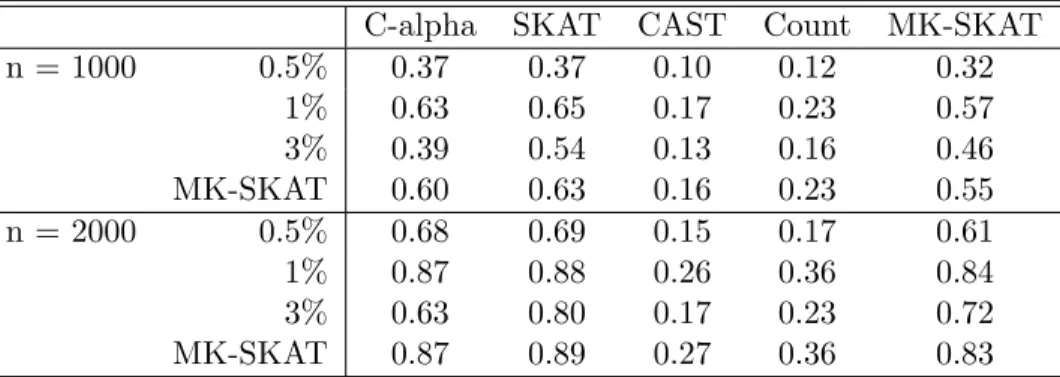
Setting 2 again examined quantitative traits and was identical to Setting 1 except the effects of the causal variants were equal to -0.5 and 0.5 with equal probability. Since the causal variants had opposing effects, this scenario favored the similarity based tests.
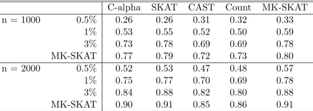
Setting 3 differed from Settings 1 and 2 in that it examineed the case where the outcome was dichotomous. Of the variants with true MAF <3%, 20% were randomly selected to be causal. All causal variants were again given equal effect size ofβ = 0.5.
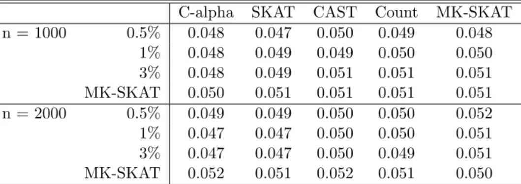
C-alpha SKAT CAST Count MK-SKAT n = 1000 0.5% 0.048 0.047 0.050 0.049 0.048
1% 0.048 0.049 0.049 0.050 0.050 3% 0.048 0.049 0.051 0.051 0.051 MK-SKAT 0.050 0.051 0.051 0.051 0.051 n = 2000 0.5% 0.049 0.049 0.050 0.050 0.052 1% 0.047 0.047 0.050 0.050 0.051 3% 0.047 0.047 0.050 0.049 0.051 MK-SKAT 0.052 0.051 0.052 0.051 0.050
Table 3.1: Type I error simulation results for quantitative traits. Each cell in the table corresponds to the type I error of SKAT using a kernel constructed based on the testing procedure at the top of the table and the grouping strategy at the left of the table. Rows and columns labeled MK-SKAT correspond to the omnibus tests across tests (with fixed group) and across groupings (with fixed test). The cells with both rows and columns labeled MK-SKAT correspond to the omnibus test across all test and groupings.
grouping strategies are optimal (since this depends on the true state of nature, which is unknown in any real data). Instead, these simulations serve to understand how MK-SKAT behaves relative to the best method and grouping strategy.
3.3 Results
3.3.1 Type I Error and Power
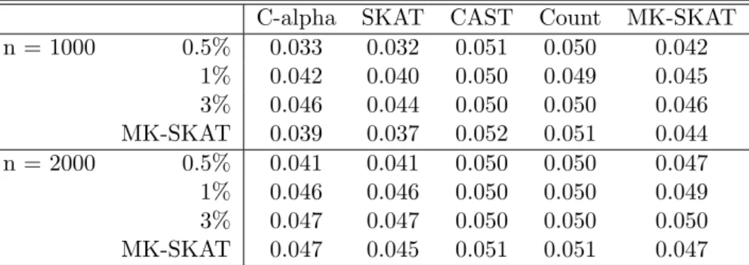
Type I error simulation results for quantitative traits and dichotomous traits are shown in Table 3.1 and Table 3.2, respectively. For quantitative traits, individual methods as well as MK-SKAT appropriately controlled the type I error at the α = 0.05 level. However, for dichotomous traits, the C-alpha test and SKAT test tended to be conservative, reflectiing previous results (Wu et al., 2011). Thus, MK-SKAT tests were conservative as well.
C-alpha SKAT CAST Count MK-SKAT n = 1000 0.5% 0.033 0.032 0.051 0.050 0.042
1% 0.042 0.040 0.050 0.049 0.045 3% 0.046 0.044 0.050 0.050 0.046 MK-SKAT 0.039 0.037 0.052 0.051 0.044 n = 2000 0.5% 0.041 0.041 0.050 0.050 0.047 1% 0.046 0.046 0.050 0.050 0.049 3% 0.047 0.047 0.050 0.050 0.050 MK-SKAT 0.047 0.045 0.051 0.051 0.047
Table 3.2: Type I error simulation results for dichotomous traits. Each cell in the table corresponds to the type I error of SKAT using a kernel constructed based on the testing procedure at the top of the table and the grouping strategy at the left of the table. Rows and columns labeled MK-SKAT correspond to the omnibus tests across tests (with fixed group) and across groupings (with fixed test). The cells with both rows and columns labeled MK-SKAT correspond to the omnibus test across all test and groupings.
group showed power would be nearly equivalent to the most powerful single kernel as well. Also, if one tested the count kernel over the 3 groupings, power would be conserved.
In Setting 2, power was dramatically decreased for the count and CAST kernels compared to Setting 1 (Table 3.4). This was due to the true model having bidirectional genetic effect on the outcome. Some rare variants increased the outcome, while some decreased the outcome. Compared to Setting 1, power was reduced for C-alpha and linear weighted kernels, but not to the same extent as count and CAST. C-alpha and linear weighted kernels applied to the variants with MAF<1% performed the best in Setting 2. MK-SKAT testing over all 12 kernels displayed power somewhat less than the most powerful single kernel, but much greater than any of the CAST or count kernels. If one applied MK-SKAT over the three groupings of the linear weighted kernel, power would be nearly equivalent to the most powerful single kernel. This setting clearly showed the adaptability of the MK-SKAT method under variation in the genotype/phenotype structure.
C-alpha SKAT CAST Count MK-SKAT
n = 1000 0.5% 0.43 0.43 0.64 0.66 0.64
1% 0.74 0.76 0.84 0.85 0.86
3% 0.47 0.64 0.63 0.63 0.71
MK-SKAT 0.69 0.72 0.81 0.85 0.84
n = 2000 0.5% 0.70 0.71 0.85 0.87 0.87
1% 0.92 0.93 0.98 0.98 0.98
3% 0.76 0.89 0.88 0.88 0.92
MK-SKAT 0.92 0.93 0.97 0.98 0.97
Table 3.3: Power results for Setting 1. Each cell in the table corresponds to the power of SKAT using a kernel constructed based on the testing procedure at the top of the table and the grouping strategy at the left of the table. Rows and columns labeled MK-SKAT correspond to the omnibus tests across tests (with fixed group) and across groupings (with fixed test). The cells with both rows and columns labeled MK-SKAT correspond to the omnibus test across all test and groupings.
C-alpha SKAT CAST Count MK-SKAT
n = 1000 0.5% 0.37 0.37 0.10 0.12 0.32
1% 0.63 0.65 0.17 0.23 0.57
3% 0.39 0.54 0.13 0.16 0.46
MK-SKAT 0.60 0.63 0.16 0.23 0.55
n = 2000 0.5% 0.68 0.69 0.15 0.17 0.61
1% 0.87 0.88 0.26 0.36 0.84
3% 0.63 0.80 0.17 0.23 0.72
MK-SKAT 0.87 0.89 0.27 0.36 0.83