THE IMPACTS OF SHORT-LIVED OZONE PRECURSORS ON CLIMATE AND AIR QUALITY
Meridith McGee Fry
A dissertation submitted to the faculty of the University of North Carolina at Chapel Hill in partial fulfillment of the requirements for the degree of Doctor of Philosophy in the
Department of Environmental Sciences and Engineering.
Chapel Hill 2013
iii Abstract
MERIDITH MCGEE FRY: The Impacts of Short-Lived Ozone Precursors on Climate and Air Quality
(Under the direction of Dr. J. Jason West)
Human emissions of short-lived ozone precursors not only degrade air quality and health, but indirectly affect climate via chemical effects on ozone, methane, and aerosols. Some have advocated for short-lived air pollutants in near-term climate mitigation strategies, in addition to national air quality programs, but their radiative forcing (RF) impacts are uncertain and vary based on emission location.
iv
photochemistry and convection. CO GWPs are fairly independent of the reduction region (GWP20: 3.71 to 4.37; GWP100: 1.26 to 1.44), while NMVOC GWPs are more variable (GWP20: -1.13 to 18.9; GWP100: 0.079 to 6.05). Accounting for additional forcings from CO and NMVOC emissionswould likely change RF and GWP estimates. Regionally-specific GWPs for NOx and NMVOCs and a globally-uniform GWP for CO may allow these gases to be included in a multi-gas emissions trading framework, and enable comprehensive strategies for meeting climate and air quality goals simultaneously.
v
Acknowledgements
I am extremely grateful to my advisor, Jason West, for his guidance, support, and dedication to my growth as a researcher. To my committee members, thank you for providing valuable insight and suggestions toward improving this work. I especially thank Vaishali Naik and Dan Schwarzkopf for your endless support with the standalone RTM. I am grateful to the NOAA Geophysical Fluid Dynamics Laboratory and UNC Research Computing for providing the necessary computational resources.
I would like to thank Bill Collins for contributing his expertise in climate metrics, and for the opportunity to collaborate on another project. I thank the Task Force on Hemispheric Transport of Air Pollution modelers, who graciously shared their data for my first study. I am also grateful to Louisa Emmons for her support with MOZART-4.
I would like to acknowledge my funding from Jason West, the U.S. EPA Science to Achieve Results Graduate Fellowship Program, and the U.S. EPA Office of Air Quality Planning and Standards. I also thank the U.S. EPA for supporting me as a summer fellow, and especially Dale Evarts, Carey Jang, and Pat Dolwick.
vi Disclaimer
vii
Table of Contents
List of Tables ... x
List of Figures ... xiii
List of Abbreviations ... xviii
Chapter 1. Introduction... 1
1.1 Policy relevance ... 3
1.2 Motivation and objectives ... 5
1.3 Table ... 8
Chapter 2. The influence of ozone precursor emissions from four world regions on tropospheric composition and radiative climate forcing ... 9
2.1 Introduction ... 9
2.2 Methodology ... 12
2.2.1 HTAP CTM simulations ... 13
2.2.2 GFDL radiative transfer model ... 15
2.3 Tropospheric composition changes ... 17
2.3.1 Tropospheric ozone changes ... 17
2.3.2 Tropospheric methane changes ... 19
2.3.3 Tropospheric sulfate changes ... 20
2.4 Radiative forcing due to precursor emission changes ... 22
2.5 Global warming potentials ... 25
2.6 Conclusions ... 28
viii
Chapter 3. Net radiative forcing and air quality responses to
regional CO emissions reductions ... 45
3.1 Introduction ... 45
3.2 Methods ... 48
3.2.1 Chemical transport modeling ... 48
3.2.2 MOZART-4 Evaluation ... 52
3.2.3 Radiative transfer modeling ... 54
3.3 Global and regional air quality responses ... 55
3.3.1 Surface CO concentrations ... 55
3.3.2 Responses of methane and ozone ... 56
3.3.3 Response of aerosols ... 58
3.4 Changes in production and export of CO and ozone ... 60
3.5 Radiative forcing and global warming potentials ... 62
3.6 Conclusions ... 65
3.7 Tables and Figures ... 70
Chapter 4. Air quality and radiative forcing impacts of anthropogenic volatile organic compound emissions from ten world regions ... 88
4.1 Introduction ... 88
4.2 Methods ... 91
4.2.1 Global chemical transport model ... 91
4.2.2 Radiative transfer model ... 93
4.3 Tropospheric composition and surface air quality ... 95
4.3.1 Methane and ozone ... 95
4.3.2 Aerosols ... 97
ix
4.5 Summary ... 102
4.6 Tables and Figures ... 106
Chapter 5. Conclusions ... 116
5.1 Scientific findings ... 116
5.2 Uncertainties and future research ... 119
5.3 Policy implications ... 123
Appendix A. The influence of ozone precursor emissions from four world regions on tropospheric composition and radiative climate forcing: Supporting material ... 127
Appendix B. Net radiative forcing and air quality responses to regional CO emission reductions: Supporting material ... 140
Appendix C. Air quality and radiative forcing impacts of anthropogenic volatile organic compound emissions from ten world regions: Supporting material ... 171
x List of Tables
Table 1.1. Summary of three dissertation studies. ... 8 Table 2.1. HTAP source-receptor sensitivity simulations, where the
four regions of reduction are East Asia, Europe, North
America, and South Asia for SR3 through SR6. ... 31 Table 2.2. Global CTMs used for multimodel mean O3, CH4, and
SO42- estimates. ... 32 Table 2.3. Multimodel mean ± 1 standard deviation reductions in
the anthropogenic emissions of NOx, NMVOC, and CO (20% of total anthropogenic emissions) among the 11
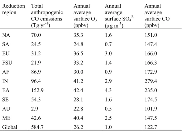
HTAP CTMs used here. ... 33 Table 3.1. For the base simulation, total anthropogenic CO
emissions by region, and regional (or global) annual average area-weighted surface O3, SO42-, and CO
concentrations. ... 70 Table 3.2. Source-receptor matrix of annual average surface CO
concentration changes (ppbv), for the regional reduction simulations, with the United States (US) also defined as a receptor in addition to the 10 regions. The largest changes for each source reduction region are in
bold. ... 71 Table 3.3. For the global and regional reduction simulations
relative to the base, global annual mean burden changes in tropospheric and upper tropospheric (UT) steady-state O3, tropospheric CH4, SO42-,NH4NO3, and SOA. The total global annual average tropospheric O3 (at steady state), SO42-, NH4NO3, and SOA burdens in the base simulation are 352 Tg O3, 1788 Gg SO42-, 457 Gg
NH4NO3, and 237 Gg SOA. ... 72 Table 3.4. For the global and regional reduction simulations, global
annual mean changes in short-term surface O3, steady-state surface O3, steady-state surface O3 per unit change in CO emissions, and long-term surface O3 per unit
change in CO emissions. ... 73 Table 3.5. Source-receptor matrix of annual average steady-state
xi
(US) also defined as a receptor in addition to the 10 regions. The largest changes for each source reduction
region are in bold. ... 74 Table 3.6. For each regional reduction, changes in global annual
average (short-term) tropospheric CO burden (BCO), and BCO per unit change in CO emissions (ECO). Also shown are CO lifetime calculated as ΔBCO / (ΔECO +
ΔPCO), the fractions of BCO change outside each reduction region and in the UT, and the changes in net CO export (XCO) from the reduction region, global CO production (PCO), and PCO outside the reduction region. The total global annual average CO burden in the base
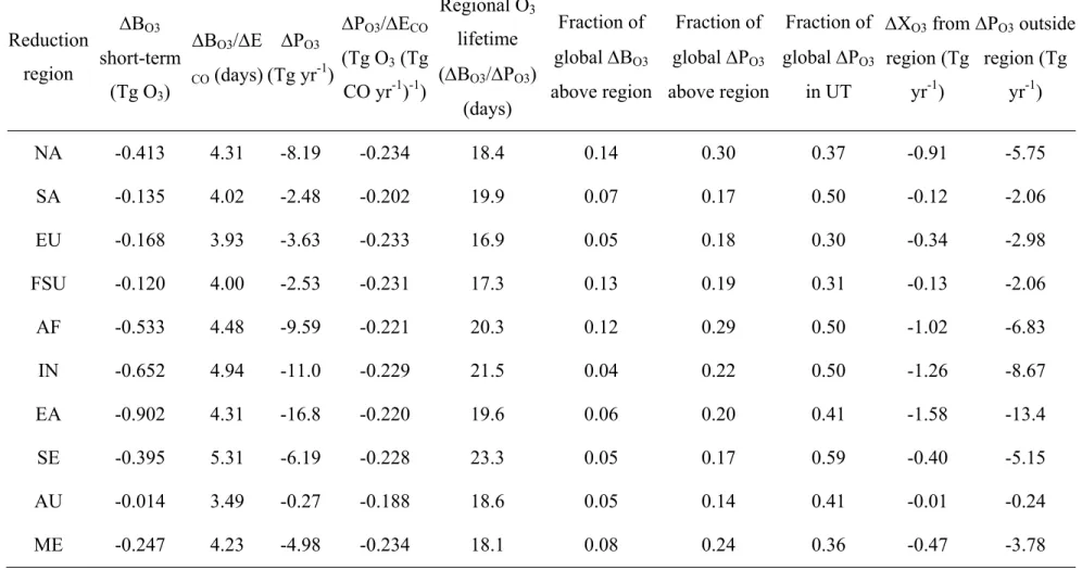
simulation is 462.6 Tg CO. ... 75 Table 3.7. Changes in global annual average (short-term)
tropospheric O3 burden (BO3), O3 production (PO3), and net O3 export (XO3) from each regional reduction, normalized per change in CO emissions (ECO), and the fractions of these above each reduction region and in the upper troposphere (UT). Regional O3 lifetimes are also shown. For the base simulation, the total global annual average O3 burden is 352.2 Tg O3, and the chemical production and loss rates are 4782.5 Tg yr-1
and 3975.0 Tg yr-1. ... 76 Table 3.8. Annual net RF globally and by latitude band (mW m-2)
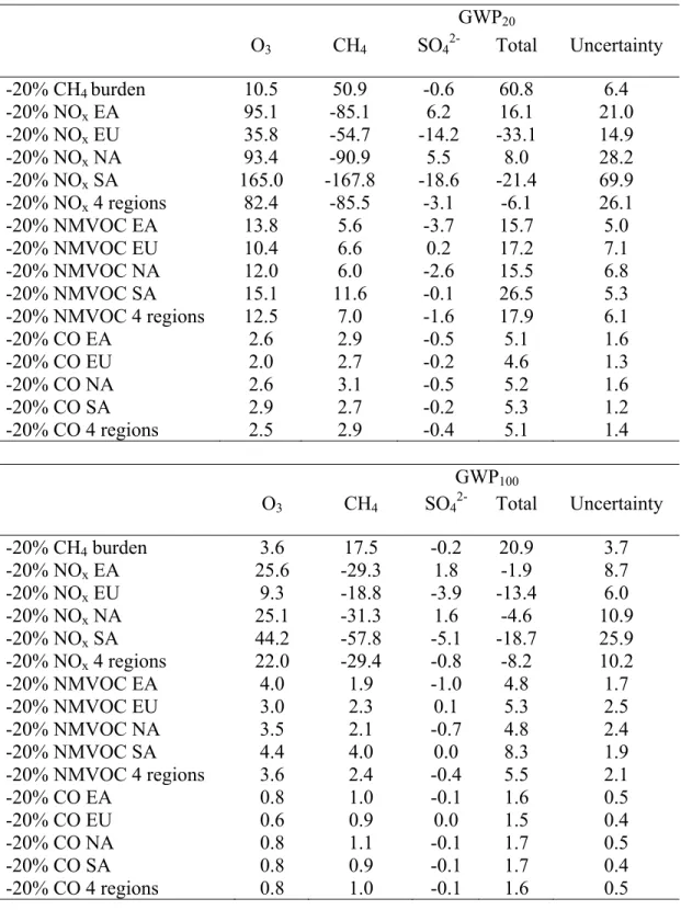
and total GWP20 and GWP100 estimates for the regional and global reduction simulations relative to the base simulation, due to changes in tropospheric steady-state O3, CH4, and SO42- concentrations. Global annual net shortwave radiation, net longwave radiation, and net RF per unit change in CO emissions (mW m-2 (Tg CO yr-1) -1) are also shown. The 10 regions estimates represent the sum of the net RFs from all 10 regional reductions;
these estimates are not directly estimated by the RTM. ... 77 Table 4.1. Changes in global annual average short-term and
steady-state tropospheric O3 burden (BO3) and tropospheric CH4 for the global and regional reductions. Changes in O3 production (PO3), PO3 normalized per unit change in NMVOC emissions (E), and PO3 outside each reduction region are shown for each regional reduction. Changes in net O3 export (XO3) from each reduction region, and the fractions of BO3 and PO3
xii
Table 4.2. For the global and regional reduction simulations relative to the base, global annual average changes in
short-term and steady-state surface O3. ... 107 Table 4.3. For the global and regional reduction simulations
relative to the base, global annual average tropospheric burden changes in SO42-,NO3- (expressedas NH4NO3), and SOA. The global annual average tropospheric SO42-, NH4NO3, and SOA burdens in the base simulation are 1785 Gg SO42-, 416 Gg NH4NO3, and
227 Gg SOA. ... 108 Table 4.4. Annual net RF globally and by latitude band (mW m-2)
and GWP20 and GWP100 estimates for the global and regional reduction simulations relative to the base, due to changes in tropospheric steady-state O3, CH4, and SO42- concentrations. Global annual net RF per unit change in NMVOC emissions (mW m-2 (Tg C yr-1)-1) is also shown. The 10 regions estimate represents the sum of the net RFs from all 10 regional reductions; this
xiii List of Figures
Figure 2.1. Global annual average changes in full (blue) and upper (yellow) tropospheric O3 burden (Tg) at steady state (perturbation minus base), where the upper troposphere is from 500 hPa to the tropopause, for the HTAP ensemble of 11 models, showing the median (black bars), mean (red points), mean ±1 SD (boxes), and max and min (whiskers), for each precursor reduction scenario (-20% global CH4 burden, and -20% regional emissions of NOx, NMVOC, CO, and combined from East Asia [EA], Europe and Northern Africa [EU],
North America [NA], and South Asia [SA]). ... 34 Figure 2.2. Global annual average changes in full (blue) and upper
(yellow) tropospheric O3 burden per change in emissions (Tg O3 / Tg emissions per year) at steady state for the individual 11 models, where the units of emissions are Tg N (for NOx), Tg C (for NMVOCs), and Tg CO (for CO), showing the median (black bars), mean (red points), mean ±1 SD (boxes), and max and
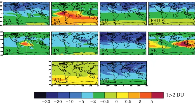
min (whiskers) across the HTAP ensemble. ... 35 Figure 2.3. Annual average steady-state tropospheric total column
O3 burden changes (10-2 DU) for the multimodel mean of 11 HTAP models, for each of the precursor reduction scenarios (-20% CH4 burden, and -20% regional emissions of NOx, NMVOC, CO, and combined). The 4 regions of reduction (NA, EU, SA,
EA) are outlined in red in the -20% CH4 plot. ... 36 Figure 2.4. Global annual multimodel changes (perturbation minus
1760 ppbv) in tropospheric CH4 (ppbv) for -20% regional emissions of NOx, NMVOC, CO, and combined: median (black bars), mean (red points), mean ±1 SD (boxes), and max and min (whiskers) for the HTAP ensemble of 11 models, estimated directly from the CH4 loss by tropospheric OH archived by each HTAP CTM (Fiore et al., 2009). Tropospheric CH4 changes were not available from INCA-vSSz for SA 20% NMVOC reduction and from LLNL-IMPACT-T5a for 20% NOx reductions (EA, EU, NA, SA); these models are excluded from the multimodel
xiv
Figure 2.5. Global annual multimodel changes (perturbation minus base) in short-term tropospheric SO42- (Gg) for -20% CH4 burden and -20% regional emissions of NOx, NMVOC, and CO: mean (red bars) and mean ±1 SD (boxes) across the HTAP ensemble of four models.
The individual model results are shown in black (+). ... 38 Figure 2.6. Annual average tropospheric total column SO42- burden
changes (g m-2) for the multimodel mean of four HTAP models for -20% CH4 burden and -20% regional emissions of NOx, NMVOC, and CO
scenarios. ... 39 Figure 2.7. a) Global annual average RF (mW m-2) for the HTAP
ensembles of 11 models (for O3 and CH4 forcing) and four models (for SO42- forcing) due to multimodel mean changes in steady-state O3, CH4, and SO42-. Vertical black bars represent the uncertainty in net RF across models, calculated as the net RF of the multimodel mean ±1 standard deviation O3 and CH4, for each perturbation (-20% CH4 burden, and -20% regional emissions of NOx, NMVOC, CO, and combined), relative to the base simulation. The uncertainty estimates for -20% CH4 account only for the variability in simulated O3 changes across the CTMs, since all CTMs uniformly reduced CH4 (1760 ppbv to 1408 ppbv). Vertical green bars represent the upper uncertainty bound of SO42- RF across models, calculated as the net RF of the multimodel mean +1 standard deviation SO42-. The RF of changes in CO2 uptake by the biosphere (yellow), are shown as a range from high to low sensitivity of vegetation to O3, estimated for a single CTM (STOCHEM) by Collins et al. (2010); these estimates are not included in the net RF (Supporting data provided in Table A1). Note the difference in scale between the -20% regional (NOx, NMVOC, CO, combined) and -20% CH4 reduction
scenarios. ... 40 Figure 2.8. Annual average net RF distributions (mW m-2),
xv
NMVOC, CO, combined) and -20% CH4 reduction
scenarios. ... 42 Figure 2.9. Radiative forcing efficiency of O3 for the 16 SR
simulations (SR3 through SR6) for the multimodel mean, showing the global, annual average O3 net RF (mW m-2), calculated as the difference between the simulated net RF due to O3 and CH4 and estimated net RF due to CH4 (Ramaswamy et al., 2001), versus the global, annual average steady-state changes in tropospheric O3 burden (Tg). The SR simulations are
distinguished by precursor (color) and region (shape). ... 43 Figure 2.10. GWPs for time horizons of a) 20 years and b) 100
years for the -20% CH4 burden and -20% regional emissions of NOx, NMVOC, and CO scenarios. The four regions estimates (labeled “All”) represent the GWP due to the sum of the four regions’ responses (to O3, CH4, SO42-, and all three species [Total GWP]). Uncertainty analysis is as in Figure 2.7, but also includes the uncertainty in the CH4 lifetimes for the base simulation (SR1) (Supporting data available in
Table A2). ... 44 Figure 3.1. Definition of 10 reduction regions. ... 79 Figure 3.2. Annual average anthropogenic CO emissions (Tg CO
yr-1) by region and sector for the base simulation, from
the RCP8.5 emissions inventory for the year 2005. ... 80 Figure 3.3. Global distribution of annual average surface CO
concentration changes (ppbv) for each of the regional reduction simulations relative to the base. The global annual average surface CO concentration changes (ppbv) for each simulation are noted in the lower right
of each panel. ... 81 Figure 3.4. Short-term and steady-state surface ozone changes as a
function of CO emissions change for each of the
regional reductions relative to the base. ... 82 Figure 3.5. Global distribution of annual average steady-state
surface O3 concentration changes (ppbv) for each of the regional reduction simulations relative to the base. The global annual average steady-state surface O3 concentration changes (ppbv) for each simulation are
xvi
Figure 3.6. Global distribution of annual average changes in tropospheric total column O3 at steady state (1e-2 DU) for each of the regional reduction simulations relative to the base. The global annual average steady-state tropospheric O3 changes (Tg O3) for each simulation
are noted in the lower right of each panel. ... 84 Figure 3.7. Global distribution of annual average changes in
tropospheric total column SO42- (g m-2) for each of the regional reduction simulations relative to the base. The global annual average tropospheric SO42- changes (Gg) for each simulation are noted in the lower right of
each panel. ... 85 Figure 3.8. Annual average net RF distributions (mW m-2) due to
changes in tropospheric steady-state O3, CH4, and SO42- for the regional and global CO reduction simulations minus the base simulation. Global annual average net RF (mW m-2) for each simulation are noted in the lower right of each panel. Note the difference in
scale between the regional and global reductions. ... 86 Figure 3.9. Global warming potentials for CO at time horizons of
20 and 100 years (GWP20, GWP100) for each regional reduction, and the contributions from short-term (O3 and SO42- changes) and long-term (long-term O3 and CH4) components. Uncertainty bars represent the average uncertainty found by Fry et al. (2012) based on the spread of atmospheric chemical models (1
standard deviation). ... 87 Figure 4.1. Global annual average surface O3 concentration
changes (ppbv) for the regional and global reduction
simulations, in the short term and at steady state. ... 111 Figure 4.2. Global distribution of annual average changes in
tropospheric total column O3 at steady state (1e-2 DU) for each of the regional reduction simulations relative
to the base. ... 112 Figure 4.3. Global distribution of annual average changes in
tropospheric total column SO42- (g m-2) for each of
the regional reduction simulations relative to the base. ... 113 Figure 4.4. Annual average net RF distributions (mW m-2) due to
xvii
SO42- for the regional and global NMVOC reduction
simulations minus the base simulation. ... 114 Figure 4.5. Global warming potentials for NMVOCs at time
horizons of 20 and 100 years (GWP20, GWP100) for the regional and global reductions, with contributions from short-term (O3 and SO42-) and long-term (O3 and CH4) components, where total GWP is short-term + long-term. Uncertainty bars represent the average uncertainty found by Fry et al. (2012) based on the spread of atmospheric chemical models (±1 standard
xviii
List of Abbreviations
AF Africa
AM2 NOAA GFDL Atmospheric Model Component of CM2 AM3 NOAA GFDL Atmospheric Model Component of CM3 AU Australia and New Zealand
ΔB Change in burden
BC Black carbon
C Carbon
CASTNET Clean Air Status and Trends Network CH4 Methane
CM3 NOAA GFDL Coupled Physical Model
CMDL Climate Monitoring and Diagnostics Laboratory CMIP5 Coupled Model Intercomparison Project Phase 5 CO Carbon monoxide
CO2 Carbon dioxide
CTM Chemical transport model CV Coefficient of variation DMS Dimethylsulfide
DU Dobson unit
ΔE Change in emissions EA East Asia
EMEP European Monitoring and Evaluation Programme EPA Environmental Protection Agency
xix F CH4 feedback factor
FSU Former Soviet Union
GEOS-5 Goddard Earth Observing System Model, version 5 GFDL Geophysical Fluid Dynamics Laboratory
Gg Gigagram
GWP Global warming potential
GWP20 Global warming potential at 20-year time horizon GWP100 Global warming potential at 100-year time horizon HNO3 Nitric acid
HO2 Hydroperoxy radical H2O2 Hydrogen peroxide hPa Hectopascal
IIASA GAINS International Institute for Applied Systems Analysis Greenhouse Gas and Air Pollution Interactions and Synergies
IMPROVE Interagency Monitoring of Protected Visual Environments IN India
IPCC Intergovernmental Panel on Climate Change
ΔL Change in loss
LM2 NOAA GFDL Land Model Component of CM2 mb Millibar
ME Middle East and Northern Africa
MEGAN Model of Emissions of Gases and Aerosols from Nature MOZART-2 Model of Ozone and Related Chemical Tracers, version 2 MOZART-4 Model of Ozone and Related Chemical Tracers, version 4
xx
g m-3 Micrograms per cubic meter
mol m-2 Micromoles per square meter mW m-2 Milliwatts per square meter
N Nitrogen
◦N Degrees North NA North America ng m-2 Nanograms per square meter ng m-3 Nanograms per cubic meter NH Northern hemisphere
NH3 Ammonia
NH4NO3 Ammonium nitrate
NMVOC Non-methane volatile organic compound
NOAA National Oceanic and Atmospheric Administration NO2 Nitrogen dioxide
NO3 Nitrate
NOx Nitrogen oxides N2O Nitrous oxide
O3 Ozone
ObjECTS GCAM Object-oriented Energy, Climate, and Technology Systems Global Change Assessment Model
OC Organic carbon OH Hydroxyl radical
ΔP Change in production
PAN Peroxyacetyl nitrate
xxi
POET Precursors of Ozone and their Effects in the Troposphere ppbv Parts per billion by volume
pptv Parts per trillion by volume
RCP Representative Concentration Pathways RCP8.5 Representative Concentration Pathway 8.5
RETRO REanalysis of the TROpospheric chemical composition over the past 40 years
RF Radiative climate forcing RO2 Peroxyl radical
RTM Radiative transfer model ◦S Degrees South
SA South Asia; South America SD Standard deviation
SE Southeast Asia SH Southern hemisphere SOA Secondary organic aerosol SO2 Sulfur dioxide
SO42- Sulfate aerosol SR Source-Receptor
STAR Science to Achieve Results
TF HTAP Task Force on Hemispheric Transport of Air Pollution
Tg Teragram
OH CH4 lifetime against loss by tropospheric OH
total Total CH4 lifetime
xxii US United States of America
UT Upper troposphere, 500 hPa to the tropopause VOC Volatile organic compound
W m-2 Watts per square meter
WMO World Meteorological Organization
Chapter 1. Introduction
Air pollution and global climate change are two leading environmental challenges facing the world today. These interrelated problems are driven by common emission sources and chemical feedbacks, and can span both near and far-reaching spatial and temporal scales (Unger et al., 2012). Many air pollutants influence climate, while climate change itself can worsen air quality (Fiore et al., 2012). In this dissertation, we focus on ozone (O3) precursors (methane [CH4], nitrogen oxides [NOx], carbon monoxide [CO], and non-methane volatile organic compounds [NMVOCs]) as an opportunity to address air pollution and global climate change together. We study the influence of O3 precursor emissions on several important short-lived air pollutants: O3 and aerosols, and climate forcers: CH4, O3, and aerosols (Pham et al., 1995; Unger et al., 2006; Shindell et al., 2009; Leibensperger et al., 2011).
2
climate impacts on emission location and chemical interactions with co-emitted species (Fiore et al., 2012). This dissertation aims to inform future policies and further the understanding of the climate and air quality effects of short-lived climate forcers.
Tropospheric O3, a secondary air pollutant and short-lived climate forcer, forms through the nonlinear photochemical oxidation of O3 precursors: CH4, CO, or NMVOCs by the hydroxyl radical (OH) in the presence of NOx. Given that the mean tropospheric lifetimes of O3 (~22 days) (Stevenson et al., 2006), CH4 (9 to 10 years), and NOx, CO, and NMVOCs (days to months) often exceed intercontinental transport times (5 to 10 days) (Fiore et al., 2009), O3 precursor emissions can affect surface and tropospheric O3 concentrations over intercontinental scales (Akimoto, 2003; TF HTAP, 2010). O3 concentrations also can respond more gradually over the long term due to changes in CH4, a longer-lived O3 precursor.
3
Tropospheric CH4 and O3 are also closely linked by precursor-driven changes in oxidants. NOx emissions tend to increase OH and hence, decrease CH4 lifetime, while CO, NMVOC, and CH4 emissions have the opposite effect, decreasing OH and increasing CH4 lifetime (Prather et al., 1995; Wild et al., 2001; Fiore et al., 2002; Naik et al., 2005; Unger et al., 2008). Through their influence on CH4, O3 precursors (including CH4 emissions themselves) also impact tropospheric O3 on the longer timescale of the CH4 lifetime (Berntsen et al., 2005; West et al., 2007).
Radiative climate forcing (RF) is one measure used to assess the influence of climate forcers (i.e. greenhouse gases and aerosols) and their precursors on the Earth’s energy balance and thus, the relative warming or cooling of climate. RF is the change in net radiation fluxes (net shortwave minus net longwave radiation) at the tropopause after allowing stratospheric temperatures to readjust to radiative equilibrium, where a positive RF implies climate warming and a negative RF indicates climate cooling. Since preindustrial times, changes in tropospheric O3 and CH4 have contributed abundance-based positive RFs of 0.35 [-0.1, +0.3] W m-2 and 0.48 ± 0.05 W m-2, approximately 21% and 31% of the RF due to CO2. In addition, tropospheric SO42-, a component of PM2.5 that scatters solar energy, has provided a negative RF of -0.40 ± 0.2 W m-2 (direct effect only) (Forster et al., 2007). O3 precursors contribute importantly to these RFs, with emissions-based estimates of 0.99 ± 0.14 W m-2 (CH4), 0.25 ± 0.04 W m-2 (CO + VOCs), and -0.29 ± 0.09 W m-2 (NOx) (Shindell et al., 2009).
1.1 Policy relevance
4
public welfare) standards for six criteria air pollutants including CO, NO2, O3, and PM2.5. These standards, however, do not take climate impacts into consideration, focusing mainly on individual air pollutant attainment in a particular area over annual time periods. The Gothenburg Protocol, adopted by the United Nations Economic Commission for Europe and amended in 2012, is one of the first multi-national agreements that moves toward addressing transboundary air pollution by setting emission reduction commitments (including for NOx, VOCs, sulfur, and ammonia) for EU member states to meet by 2020 and beyond. Existing air pollution legislation, however, will likely be inadequate to address rising O3 and PM2.5 levels worldwide, which will continue to harm human health and the environment, despite the downward trend of O3 levels in the U.S. and Europe. Developing nations, in particular, may lack the experience needed to implement future air pollution control policies (Dentener et al., 2006). As a result, more stringent emissions control measures will be needed to ensure a sustainable atmospheric environment in the future.
5
Over the past decade, several studies have suggested that short-lived climate forcers and their precursors be included in climate agreements like the Kyoto Protocol (Fuglestvedt et al., 1999; Rypdal et al., 2005, 2009; Naik et al., 2005; Unger et al., 2008; Fry et al., 2012), as a way to address climate change in the coming decades and to complement longer term CO2 mitigation efforts (Jackson et al., 2009; Shindell et al., 2012; Unger et al., 2012). Reducing certain short-lived climate forcers also provides important benefits to human health and the environment, as O3 and PM2.5 exposure have been linked to adverse respiratory and cardiovascular health effects, premature mortality, and ecosystem damages. However, short-lived species including O3 precursors (apart from CH4) impact RF non-uniformly and can contribute to both climate warming and cooling, making it difficult to identify different regions’ contributions to global climate change. As a result, geographically-varying GWPs may be needed (Fuglestvedt et al., 1999; Wild et al., 2001; Berntsen et al., 2005; Naik et al., 2005; West et al., 2007; Derwent et al., 2008), in contrast to long-lived greenhouse gases (e.g. CO2) whose more uniform RF impacts allow for globally-uniform GWPs. There is a need to more fully understand the effects of O3 precursors on the distributions of O3, SO42-, and other secondary species, and the corresponding variability in RF and GWP estimates (Berntsen et al., 2005). Future mitigation efforts will likely need to consider air quality and global climate change together, as many air pollutants and climate forcers originate from the same precursors and emission sources (Unger et al, 2012).
1.2 Motivation and objectives
6
reductions (Fuglestvedt et al., 1999; Wild et al., 2001; Berntsen et al., 2005; Naik et al., 2005; West et al., 2007; Derwent et al., 2008), finding that O3 concentrations and RF depend considerably on the location or sector of NOx emissions, with greater sensitivity to emissions from the tropics. One global model’s results show that NOx emission reductions from 9 world regions produce overall positive global net RFs (Naik et al., 2005), while West et al. (2007) found that global reductions in CH4, CO, and NMVOCs result in negative net RFs. Naik et al. (2005) also analyzed reductions in NOx, CO, and NMVOC emissions together from 3 regions, and Berntsen et al. (2005) evaluated CO emissions changes from 2 regions.
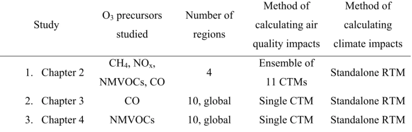
This dissertation examines the air quality, tropospheric burden, and RF impacts of individual O3 precursor emission reductions through three separate studies (Table 1.1). The first study aims to evaluate O3 precursor emissions from 4 regions across an ensemble of 11 global chemical transport models (CTM) that participated in the Task Force on Hemispheric Transport of Air Pollution multimodel intercomparison of Source-Receptor sensitivity (Chapter 2). This study improves upon previous methods by providing the spread in tropospheric burden and RF estimates across multiple CTMs as an indicator of model uncertainty, and by differentiating the contributions of O3, CH4, and SO42- to global net RF and GWP using a radiative transfer model (RTM). The RF and GWP estimates for each precursor are compared among the 4 regions and to previous studies, improving our understanding of the sensitivity to different regions’ emissions.
7
8 1.3 Table
Table 1.1. Summary of three dissertation studies.
Study O3 precursors studied
Number of regions
Method of calculating air quality impacts
Method of calculating climate impacts 1. Chapter 2 CH4, NOx,
NMVOCs, CO 4
Ensemble of
Chapter 2. The influence of ozone precursor emissions from four world regions on tropospheric composition and radiative climate forcing1
2.1 Introduction
Tropospheric ozone (O3), methane (CH4), and aerosols make important contributions to the global mean radiative forcing (RF) of climate (Forster et al., 2007; Ramaswamy et al., 2001). Here we aim to quantify the net RF of these species due to regional changes in O3 precursor emissions, across an ensemble of global chemical transport models (CTMs). We define net RF as the net (incoming minus outgoing) change in irradiance (solar and infrared) at the tropopause between a base and perturbed state (in Watts per square meter [W m-2]) after allowing stratospheric temperatures to readjust (Forster et al., 2007). The contribution of changes in tropospheric O3 to the global mean RF since preindustrial times is an estimated 0.35 ±0.15 Wm-2, which is approximately 21% of the RF due to changes in carbon dioxide (CO2) (Forster et al., 2007). Changes in CH4 have contributed approximately 0.48 Wm-2, while those in sulfate aerosols (SO42-) have contributed approximately -0.4 ±0.2 Wm-2 (direct effect only) (Forster et al., 2007).
Changes in O3 precursor emissions (nitrogen oxides [NOx], non-methane volatile organic compounds [NMVOC], carbon monoxide [CO], and CH4) affect the abundance
1
10
of gaseous species (O3 and CH4), and aerosols via changes in the availability of atmospheric oxidants (hydroxyl radical [OH], hydrogen peroxide [H2O2], O3) (Pham et al., 1995; Unger et al., 2006; Shindell et al., 2009; Leibensperger et al., 2011). These perturbations in turn influence the RF due to O3 and CH4 and inorganic aerosol-phase species (Ming et al., 2005; Unger et al., 2006; Naik et al., 2007; Shindell et al., 2009). O3 precursors also affect organic aerosols, including the formation of secondary organic aerosols (SOA) (Carlton et al., 2010), but the resulting RF remains to be quantified. O3 decreases plant growth and hence reduces the removal of CO2 from the atmosphere (Felzer et al., 2007; Sitch et al., 2007; Collins et al., 2010), while NOx emissions influence nitrogen deposition and the subsequent uptake of CO2 in terrestrial and oceanic ecosystems (Holland and Lamarque, 1997; Duce et al., 2008). Because of these influences, actions to control O3 precursor emissions affect both air quality and global climate (Fiore et al., 2002; Dentener et al., 2005; West et al., 2007).
11
negative RF of the O3 precursors, mainly due to direct reductions in CH4 forcing (Fiore et al., 2002; Shindell et al., 2005; West et al., 2007).
12
Here we investigate the effects of a 20% reduction in global CH4 abundance and 20% reductions in anthropogenic emissions of NOx, NMVOC, and CO, individually and combined, from four world regions on tropospheric O3, CH4, and SO42- concentrations and on the resulting distribution and magnitude of global net RF for all precursor-region pairs. We use results from an ensemble of global CTMs that participated in the Task Force on Hemispheric Transport of Air Pollution (TF HTAP) multimodel intercomparison study of Source-Receptor (SR) sensitivity (Fiore et al., 2009), which allows for an assessment of uncertainty as the spread across CTMs. We examine the regional dependency of RF and global warming potential (GWP) to individual precursors by comparing estimates across the four regions of reduction.
2.2 Methodology
13
2.2.1 HTAP CTM simulations
The SR simulations performed by each CTM are outlined in Table 2.1. We analyze O3 and CH4 results from 11 CTMs and SO42- results from four CTMs (Table 2.2). Each CTM utilized its own emissions inventory and prescribed meteorological fields for the year 2001 (Fiore et al., 2009). Anthropogenic emissions of NOx, NMVOCs, CO, and all precursors combined were reduced by 20% in each of four world regions: East Asia (EA), Europe and Northern Africa (EU), North America (NA), and South Asia (SA). For CH4, the present-day abundance (1760 parts per billion by volume [ppbv]) was imposed in all simulations except for the CH4 control simulation (SR2), where global CH4 abundance was decreased by 20% to 1408 ppbv. All simulations were performed for a full year (2001), after an initial spin-up of at least six months (Fiore et al., 2009).
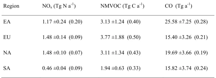
The multimodel mean ±1 standard deviation changes in the anthropogenic emissions of NOx, NMVOCs, and CO, across 11 CTMs, are presented in Table 2.3. There is considerable variability in the emission reduction magnitudes across CTMs. Coefficients of variation (CVs) (standard deviation / mean) are lowest for NOx emissions from EU, NA, and SA, while there is more variability in NMVOC and CO emissions from the four regions, consistent with the comparison of current global emission inventories by Granier et al. (2011).
14
2001, but overestimated measurements by more than 10 ppb during the summer and fall over the eastern United States and Japan. Jonson et al. (2010) compared simulated vertical O3 profiles with observed ozonesonde profiles, finding that the spread in CTM results (and their over and underestimation of O3 soundings) increases in the spring and summer with more active chemistry. In the winter and spring, seasonal averages for most CTMs were within 20% of sonde measurements in the upper and middle troposphere. Simulated SO42- concentrations at the surface for the base simulation (SR1) also have been compared to observations (M. Schulz, personal communication, 2011, preliminary results available at http://aerocom.met.no/cgi-bin/aerocom/surfobs_annualrs.pl), where the results show that the CTMs are generally realistic.
Short-lived O3 precursors affect tropospheric O3 within hours to weeks after their emission; however, they also affect OH, which influences the lifetime of CH4 and in turn, O3 in the long term (Prather et al., 1996; Wild et al., 2001; Berntsen et al., 2005; Naik et al., 2005). Global CH4 changes were calculated by Fiore et al. (2009), based on the CH4 loss by tropospheric OH diagnostic reported for each CTM and SR3 through SR6, relative to the fixed CH4 abundance of 1760 ppbv. Long-term O3 responses are then calculated in each grid cell, following West et al. (2007, 2009b), by scaling the change in O3 from the CH4 control simulation (SR2 minus SR1) to the calculated global CH4 change for each SR simulation and CTM. We then add the long-term O3 responses to the simulated short-term O3 responses to give O3 concentrations at steady state.
15
tropospheric O3 concentrations for each simulation and CTM. Stratospheric O3 is taken for the year 2001 from the AC&C/SPARC O3 database prepared for CMIP5 (Available: http://pcmdi-cmip.llnl.gov/cmip5/forcing.html). Søvde et al. (2011) found that around 15% of the RF from O3 precursors is due to O3 changes in the lower stratosphere, using a single model with both standard and updated chemistry. Since we ignore lower stratospheric O3 changes, our RF estimates may underestimate the full effect of O3 precursors. After each CTM’s O3 and SO42- results are interpolated to a common resolution (longitude x latitude x level) as required by the RTM (72 x 37 x 33 for O3; 96 x 80 x 14 for SO42-), the HTAP ensemble mean ±1 standard deviation O3 and SO4 2-distributions are calculated in each grid cell and month in three dimensions, in addition to the ensemble mean ±1 standard deviation global CH4 abundances (derived from the CH4 loss by tropospheric OH diagnostics). Global O3, CH4, and SO42- changes are calculated for each CTM as perturbation (SR2 to SR6) minus base (SR1) values.
2.2.2 GFDL radiative transfer model
16
update well-mixed greenhouse gas concentrations based on observations for the year 2001 included as part of the historical period (1750-2005) of the CMIP5 Representative Concentration Pathways (RCP) database (Meinshausen et al., 2011) (Available: http://www.iiasa.ac.at/web-apps/tnt/RcpDb/dsd?Action=htmlpage&page=download). We also update the solar data used by the RTM to the CMIP5 solar forcing data (Available: http://www.geo.fu-berlin.de/en/met/ag/strat/forschung/SOLARIS/Input_data/CMIP5_solar_irradiance.html). The RTM simulations do not include the indirect effects of aerosols on clouds or the internal mixing of aerosols. RF contributions from changes in nitrate aerosols, changes in stratospheric O3 and water vapor, changes to the carbon cycle via O3 and nitrogen deposition, and changes to CO2 from CH4, CO, and NMVOC oxidation are also omitted in the RTM simulations.
17 2.3 Tropospheric composition changes
2.3.1 Tropospheric ozone changes
Figure 2.1 shows the changes in global annually averaged steady-state tropospheric O3 burden and its variability across 11 HTAP CTMs. Full troposphere and upper troposphere (UT) O3 burdens are distinguished because O3 in the UT has a higher RF efficiency on a per molecule basis (Lacis et al., 1990; Wang et al., 1993; Forster and Shine, 1997). For each CTM’s regridded O3 distributions that have been blended with CMIP5 stratospheric O3 values (section 2.1), the UT is defined from 500 hPa to the tropopause, where the tropopause is identified at the 150 ppbv O3 level.
The largest changes in full troposphere and UT O3 burden are found for the 20% CH4 reduction, followed by the 20% combined precursor reductions from NA and EA, respectively. However, there is considerable diversity among the 11 CTMs’ estimates of full troposphere and UT O3 burden changes. In these 17 SR simulations relative to the base case, the change in UT O3 burden per change in full troposphere O3 burden (UT O3 / full troposphere O3) is largest for reductions in global CH4 (0.36 to 0.47) and regional CO emissions (0.19 to 0.53), and smallest for regional NMVOC reductions (0.16 to 0.42) across the 11 CTMs, reflecting the longer lifetimes of CO and CH4 in comparison to NMVOCs and NOx. UT O3 / full troposphere O3 is also largest for individual O3 precursor (NOx, NMVOC, and CO) reductions from SA in comparison to the other regions.
18
change in full troposphere and UT O3 burden per change in emissions out of the four regions, which can be attributed to more rapid vertical mixing, stronger photochemistry, and greater sensitivity of O3 to precursor emissions from the tropics and southern hemisphere (SH) (Kunhikrishnan et al., 2004; West et al., 2009a). We find less variability across the four regions in reducing full troposphere and UT O3 burden per change in NMVOC and CO emissions (Figure 2.2), but six CTMs show that SA NMVOC and CO reductions produce the largest reductions in UT O3 burden per change in emissions.
long-19
range O3. Across the 11 CTMs, we find that tropospheric PAN decreases are correlated to the changes in NMVOC emissions for the EA, EU, and NA reductions.
2.3.2 Tropospheric methane changes
Although global CH4 was held constant by each CTM in all perturbations, we analyze the changes in global tropospheric CH4 calculated off-line for each perturbation. NOx reductions from all four regions increase global CH4 abundance via decreases in OH, while NMVOC and CO reductions from all four regions decrease global CH4 (Figure 2.4). These changes in CH4 drive the long-term O3 changes discussed in the previous section. For particular precursors, reductions from certain regions, e.g. CO reductions from EA, are slightly more effective at decreasing global CH4 than other regions. However, there is noticeable variability among the CTMs’ changes in global CH4 (Figure 2.4), which is partly explained by variance in CTM emissions for CO, but not for NOx and NMVOCs.
For several CTMs, some emissions perturbations had minimal impact on global OH, resulting in calculated steady-state CH4 changes of zero. In addition, the CVs of CH4 change are lowest in magnitude for NOx reductions (0.22 to 0.39) and highest for NMVOC reductions (-0.40 to -1.12), perhaps reflecting differing NMVOC speciation and chemical schemes among the CTMs (Collins et al. 2002).
20
from individual precursor reductions, while global CH4 changes from EA and EU combined precursor reductions are slightly negative in contrast to small positive global CH4 changes from the sum. The three (of 11) CTMs that did not include reductions in SO2 and aerosols in the SR6 experiments (Fiore et al., 2009) show global CH4 changes from the combined precursor reductions close to the sum of CH4 changes from individual NOx, NMVOC, and CO reductions. This suggests that deviations from additivity may be due to reductions in SO2 and aerosols (in SR6) affecting CH4.
2.3.3 Tropospheric sulfate changes
There is considerable variability and disagreement in the sign of SO42- responses among the four CTMs evaluated (Figure 2.5). The greatest variability in global SO4 2-burden across the CTMs occurs for the CH4 reduction and for NOx reductions from all four regions. There is less variability across CTMs for NMVOC and CO reductions, but still differences in the sign of change.
21
Figure 2.5 shows that the sign of SO42- response is not consistent across all four CTMs, suggesting uncertainty in the modeled effects of O3 precursors on oxidants, the relative importance of these oxidation pathways, and the lifetime and removal of SO2 and SO42-.
22
2.4 Radiative forcing due to precursor emission changes
Figure 2.7 (and Table A1) show the global annual net RF due to O3, CH4, and SO42-, estimated from RTM simulations, first for multimodel mean O3 and CH4, and second for multimodel mean O3, CH4, and SO42-, for each SR scenario relative to the base case. We calculated the net RF distributions for each perturbation scenario (SR2 through SR6) by subtracting (in each grid cell and month) the simulated radiative fluxes for the base case (SR1) from those for each perturbation. To estimate the contribution of the multimodel mean SO42- to the global annual net RF, we subtracted the net RF results due to O3 and CH4 from the net RF due toO3, CH4, and SO42- for each SR scenario, assuming the effects of O3, CH4, and SO42- are additive. To distinguish the contributions of O3 and CH4 to the global annual net RF, we estimated the net RF due to the multimodel mean CH4 for each SR scenario, using the formula of Ramaswamy et al. (2001), attributing the difference to O3 RF.
Computational limitations prevented us from simulating the RFs individually for each CTM’s 18 SR scenarios. Instead, we simulate RFs for multimodel means, and for the multimodel mean ±1 standard deviation O3 and CH4 and the multimodel mean +1 standard deviation SO42- to account for uncertainty in the net RF due to differences in the CTMs. We show uncertainty (mean ±1 standard deviation) for the resulting net RF, which includes the uncertainty in O3 and CH4 RFs, as changes in O3 and CH4 are not strongly correlated among the 11 CTMs for most scenarios (Figure A4). For NOx
23
deviation O3 and the multimodel mean -1 standard deviation CH4 (and the reverse) to estimate uncertainty.
Figure 2.7 shows that O3 and CH4 RFs have the same sign as the tropospheric composition changes in section 3; since SO42- is cooling, SO42- RF has the opposite sign. NOx reductions from all four regions produce an overall positive net RF due to increases in CH4, which outweigh the negative net RF due to decreases in O3 (Figure 2.7a). Negative global net RFs are produced by CO and NMVOC reductions, due to O3 and CH4 decreases, and also by the combined precursor reductions, as increases in CH4 from NOx reductions roughly cancel CH4 decreases from NMVOC and CO reductions (Fiore et al., 2009). The net RF due to the combined precursor reduction is 98% to 117% of the sum of the net RFs (of O3 and CH4) due to reductions of each individual precursor, across the four regions, showing approximate additivity for the different precursors.
Consistent with the SO42- changes in Figure 2.5, NOx reductions from EU and SA contribute a positive SO42- RF, while EA and NA NOx reductions produce negative SO4 2-RF. The SO42- RFs for NMVOC and CO reductions vary in magnitude and sign across the four regions, corresponding to the disagreement in SO42- response across the CTMs (Figure 2.5). We do not estimate the contribution of SO42- to net RF for the combined reductions, since many of these perturbations included 20% reductions in SO2 and aerosols, making it difficult to isolate the effect of NOx, NMVOC, and CO on SO42- RF.
24
converted to equilibrium responses by integrating over 100 years. The range of CO2 RF represents high to low sensitivity of vegetation to O3. With the additional consideration of CO2 RF, the global annual net RF due to regional NOx reductions changes sign to an overall net climate cooling (-0.83 to -4.28 mWm-2 for all four regions), while the negative net RFs for regional NMVOC and CO reductions are reinforced by the addition of CO2 RF (Table A1).
We normalize the global annual net RF estimates (Figure 2.7a) by each region’s reduction in emissions (Table 2.3). The net RF per unit change in NOx and NMVOC emissions is greatest for SA reductions out of the four regions (Figure 2.7b), corresponding to the sensitivity findings in section 3.1. For CO reductions, all four regions are approximately as effective at reducing global net RF per unit CO emissions, consistent with CO’s longer atmospheric lifetime.
25
increases globally, but in the NH these positive RFs are outweighed by the negative RF of O3 decreases (Figure 2.8). For CH4, NMVOC, CO, and combined reductions, negative net RFs from O3 decreases in the NH overlay negative RFs globally due to CH4. While Figure 2.7 presents globally averaged forcings, the regionally inhomogeneous forcings in Figure 2.8 are also relevant for regional climate change (Shindell and Faluvegi, 2009). However, regional RF patterns resulting from changes in tropospheric loadings do not directly translate to regional climate responses (Levy et al., 2008; Shindell et al., 2010).
In Figure 2.9, the relationship between tropospheric O3 burden changes and global O3 RF is strongly linear, giving a RF efficiency of approximately 3.27 mW m-2 per Tg O3 or 35.6 mWm-2 DU-1 (1 DU ≈ 10.88 Tg O3 [Park et al., 1999]). This efficiency compares well with those estimated in previous studies, 34 to 48 mWm-2 DU-1 (Hauglustaine and Brasseur, 2001; Wild et al., 2001; Fiore et al., 2002) and 23 mWm-2 DU-1 (for NOx) and 43 mWm-2 DU-1 (for CH4 and CO+VOCs) (Shindell et al., 2005). Here reductions from EU and NA (with exception of NA NOx) fall at or above the average RF efficiency line, suggesting lower RF efficiency. EA and SA reductions (except for EA NMVOC) have RF efficiency greater than average, as these regions have greater influences on the UT where RF is the most efficient (Lacis et al., 1990; Wang et al., 1993; Forster and Shine, 1997; West et al., 2009a).
2.5 Global warming potentials
26
metrics have been proposed to compare climate effects, such as the global temperature potential (GTP) (Shine et al., 2005; 2007), none are as widely used as the GWP. We choose to analyze the GWP here for comparison with earlier studies.
The basis for the GWP calculation is the integrated RF following a pulse emission. In section 4, O3 RF was calculated for equilibrium conditions for the sum of the short and long-term O3 responses (Figure 2.7 and Table A1). Here long-term O3 RF is calculated by scaling O3 RF from SR2 by the ratio of steady-state O3 burden change in a particular SR scenario (SR minus base) to those of SR2 (SR2 minus base). The short-term O3 RF is then the difference between the steady-state RF (section 4) and long-term RF. Following Collins et al. (2010), RF as a function of time is calculated for a one-year emissions perturbation, for each SR scenario. The short-term RF components (SO42- and short-term O3) are assumed to be constant over the one-year pulse and then drop to zero instantaneously; whereas, the long-term components (CH4 and long-term O3) respond and decay with the multimodel mean CH4 perturbation lifetime (11.65 years). For the 20% CH4 reduction (SR2), an analytical expression is used to calculate the impact of a one-year emissions pulse and subsequent decay (Collins et al., 2010). This CH4 perturbation is used to scale the SO42- and O3 RFs from SR2 in Figure 2.7. The formula by Ramaswamy et al. (2001) is used to calculate the CH4 RF.
27
the GWPs. The patterns of GWP100 are very similar to the normalized forcings in Figure 2.7b (the patterns would be identical for GWP∞), whereas the GWP20 patterns give more emphasis to short-lived O3 and SO42- than GWP100. For NOx emissions, this brings GWP20 proportionally closer to zero.
28
For NOx and NMVOCs, SA emissions have a larger impact than emissions from the other regions. This suggests that some latitudinal dependence may be appropriate for GWPs of O3 precursors. Note that equatorial or SH emission changes were not considered in this study, but Fuglestvedt et al. (2010) found a dependence on latitude. European NOx emissions have a more negative GWP than other regions in the northern mid-latitudes, as O3 production in this NOx-saturated region is lower.
2.6 Conclusions
We quantify the magnitude and distribution of global net RF due to changes in O3, CH4, and SO42- for 20% reductions in global CH4 and regional NOx, NMVOC, CO, and combined precursor emissions. We find that the 20% NOx reductions produce global, annually averaged positive net RFs, as positive CH4 RFs outweigh negative O3 RFs, consistent with previous studies (Fuglestvedt et al., 1999; Wild et al., 2001; Naik et al., 2005; West et al., 2007). For CH4, NMVOC, and CO reductions, O3 and CH4 RFs are synergistic, yielding overall negative net RFs, consistent with previous global-scale studies (Fiore et al., 2002; West et al., 2007; Shindell et al., 2009). Including the effects of O3 on plant growth and the carbon cycle may change the sign of net RF for NOx reductions to an overall net climate cooling, in contrast to previous results that neglect this effect, while reinforcing the negative net RFs due to NMVOC and CO reductions, but future research is needed to better quantify this effect.
29
NMVOC) are greatest for SA reductions. RF is more uniformly sensitive to CO emission reductions from each of the four regions, which agrees with O3 burden changes per unit CO being less variable across the four regions. The trends in GWP100 across the four regions, for each precursor, reflect the normalized net RF results. Compared to GWP100, the GWP20 patterns are influenced more by short-term O3 and SO42-. The large uncertainties in the NOx GWP estimates, mainly from the variation in calculated CH4 responses across the CTMs, limit the determination of the sign of NOx GWPs. The estimated GWPs for individual regions are from the largest model ensemble that has been analyzed to date, and are broadly comparable to previous studies.
We find that regional RFs correspond to localized increases and decreases in SO42- burden. O3 changes are most important for RF on the regional to hemispheric scales, and CH4 influences RF globally, dominating the RF response in the SH. The estimated contribution of SO42- (direct effect only) to net RF is small compared to the RF of O3 and CH4. Shindell et al. (2009) found with a single CTM that for global NOx, CO, and VOC emissions, changes in SO42- contributed a RF more comparable in magnitude to the RFs of O3 and CH4. Our findings contrast with those of Shindell et al. (2009) on the importance of SO42- RF due to O3 precursors. However, the robustness of these results is limited, since there was substantial variability in SO42- among only four HTAP CTMs. The effects of O3 precursors on SO42- via oxidants merit further research, using newer models that include improved treatment of oxidant-aerosol interactions.
30
while we capture the most important forcings, a more complete analysis of RF could include RFs due to changes in nitrate aerosols (likely important for NOx reductions), the indirect effect of aerosols, internal mixing of aerosols, changes in stratospheric O3 and water vapor, and changes to the carbon cycle via nitrogen deposition. Finally, we estimate RF due to changes in the radiative budget of the global atmosphere, but do not estimate the full climate response to regional forcings. Future research should link global and regional RF to climate responses.
31 2.7 Tables and Figures
Table 2.1. HTAP source-receptor sensitivity simulations, where the four regions of reduction are East Asia, Europe, North America, and South Asia for SR3 through SR6.
Scenario Description
SR1 Base simulation
SR2 20% reduction in global CH4 mixing ratio SR3 20% reduction in regional NOx emissions SR4 20% reduction in regional NMVOC emissions SR5 20% reduction in regional CO emissions
32
Table 2.2. Global CTMs used for multimodel mean O3, CH4, and SO42- estimates. Model Institution
CAMCHEM-3311m13a NCAR, USA FRSGCUCI-v01 Lancaster University, UK GISS-PUCCINI-modelE NASA GISS, USA GMI-v02f NASA GSFC, USA
INCA-vSSz LSCE, France
LLNL-IMPACT-T5aa LLNL, USA MOZARTGFDL-v2a GFDL, USA
MOZECH-v16 FZ Juelich, Germany STOC-HadAM3-v01 University of Edinburgh, UK
TM5-JRC-cy2-ipcc-v1a JRC, Italy
UM-CAM-v01 University of Cambridge, UK/NIWA, NZ
a The four global CTMs used for multimodel mean SO
33
Table 2.3. Multimodel mean ± 1 standard deviation reductions in the anthropogenic emissions of NOx, NMVOC, and CO (20% of total anthropogenic emissions) among the 11 HTAP CTMs used herea.
Region NOx (Tg N a-1) NMVOC (Tg C a-1) CO (Tg a-1) EA 1.17 ±0.24 (0.20) 3.13 ±1.24 (0.40) 25.58 ±7.25 (0.28) EU 1.48 ±0.14 (0.09) 3.77 ±1.88 (0.50) 15.40 ±3.26 (0.21) NA 1.48 ±0.10 (0.07) 3.11 ±1.34 (0.43) 19.69 ±3.66 (0.19) SA 0.46 ±0.04 (0.09) 1.94 ±0.63 (0.33) 15.82 ±3.74 (0.24)
34
Figure 2.1. Global annual average changes in full (blue) and upper (yellow) tropospheric O3 burden (Tg) at steady state (perturbation minus base), where the upper troposphere is from 500 hPa to the tropopause, for the HTAP ensemble of 11 models, showing the median (black bars), mean (red points), mean ±1 SD (boxes), and max and min (whiskers), for each precursor reduction scenario (-20% global CH4 burden, and -20% regional emissions of NOx, NMVOC, CO, and combined from East Asia [EA], Europe and Northern Africa [EU], North America [NA], and South Asia [SA]).
-20% NOx -20% NMVOC -20% CO -20% Combined -20% CH4
-2.5 -2.0 -1.5 -1.0 -0.5 0.0
EA EU NA SA EA EU NA SA EA EU NA SA EA EU NA SA
Δ
T
ropospheric
Ozone
Burden
(Tg)
35
Figure 2.2. Global annual average changes in full (blue) and upper (yellow) tropospheric O3 burden per change in emissions (Tg O3 / Tg emissions per year) at steady state for the individual 11 models, where the units of emissions are Tg N (for NOx), Tg C (for NMVOCs), and Tg CO (for CO), showing the median (black bars), mean (red points), mean ±1 SD (boxes), and max and min (whiskers) across the HTAP ensemble.
-2.0 -1.6 -1.2 -0.8 -0.4 0.0
EA EU NA SA
-0.20 -0.16 -0.12 -0.08 -0.04 0.00
EA EU NA SA
-0.04 -0.03 -0.02 -0.01 0.00
EA EU NA SA
Δ
T
ropospheric Ozone per
Δ
Emissions
(Tg ozone /
Tg emissions per year)
36
Figure 2.3. Annual average steady-state tropospheric total column O3 burden changes (10-2 DU) for the multimodel mean of 11 HTAP models, for each of the precursor reduction scenarios (-20% CH4 burden, and -20% regional emissions of NOx, NMVOC, CO, and combined). The 4 regions of reduction (NA, EU, SA, EA) are outlined in red in the -20% CH4 plot.
-20% NO
EA EU NA SA
-20% NMVOC
-20% CO
-20% Combined
-20% CH4
10 DU-2
37
Figure 2.4. Global annual multimodel changes (perturbation minus 1760 ppbv) in tropospheric CH4 (ppbv) for -20% regional emissions of NOx, NMVOC, CO, and combined: median (black bars), mean (red points), mean ±1 SD (boxes), and max and min (whiskers) for the HTAP ensemble of 11 models, estimated directly from the CH4 loss by tropospheric OH archived by each HTAP CTM (Fiore et al., 2009). Tropospheric CH4 changes were not available from INCA-vSSz for SA 20% NMVOC reduction and from LLNL-IMPACT-T5a for 20% NOx reductions (EA, EU, NA, SA); these models are excluded from the multimodel CH4 changes for these perturbations.
-15 -10 -5 0 5 10 15 20
EA EU NA SA EA EU NA SA EA EU NA SA EA EU NA SA
Δ
T
roposp
h
eri
c Methane
(ppbv)
38
Figure 2.5. Global annual multimodel changes (perturbation minus base) in short-term tropospheric SO42- (Gg) for -20% CH4 burden and -20% regional emissions of NOx, NMVOC, and CO: mean (red bars) and mean ±1 SD (boxes) across the HTAP ensemble of four models. The individual model results are shown in black (+).
-6 -4 -2 0 2 4 6
EA EU NA SA EA EU NA SA EA EU NA SA
Δ
T
ropospheric
Sulfate Burden (Gg)
-16 -12 -8 -4 0 4
39
Figure 2.6. Annual average tropospheric total column SO42- burden changes (g m-2) for the multimodel mean of four HTAP models for -20% CH4 burden and -20% regional emissions of NOx, NMVOC, and CO scenarios.
-20% NO
-20% NMVOC
-20% CO
-20% CH
EA EU NA
μg m−2
4 x
40
Figure 2.7. a) Global annual average RF (mW m-2) for the HTAP ensembles of 11 models (for O3 and CH4 forcing) and four models (for SO42- forcing) due to multimodel mean changes in steady-state O3, CH4, and SO42-. Vertical black bars represent the uncertainty in net RF across models, calculated as the net RF of the multimodel mean ±1 standard deviation O3 and CH4, for each perturbation (-20% CH4 burden, and -20% regional emissions of NOx, NMVOC, CO, and combined), relative to the base simulation. The uncertainty estimates for -20% CH4 account only for the variability in simulated O3 changes across the CTMs, since all CTMs uniformly reduced CH4 (1760 ppbv to 1408 ppbv). Vertical green bars represent the upper uncertainty bound of SO42- RF across models, calculated as the net RF of the multimodel mean +1 standard deviation SO42-. The RF of changes in CO2 uptake by the biosphere (yellow), are shown as a range from high to low sensitivity of vegetation to O3, estimated for a single CTM (STOCHEM) by Collins et al. (2010); these estimates are not included in the net RF (Supporting data
-6 -4 -2 0 2 4 6 8
EA EU NA SA
G lobal A nnual N et RF / Δ E m issions (m W m -2 / T g em issions per y ear) -1.2 -0.8 -0.4 0.0 0.4 0.8
EA EU NA SA
-20% NOx -20% NMVOC
-0.2 -0.1 0.0 0.1
EA EU NA SA
Methane RF/emissions Ozone RF/emissions Sulfate RF/emissions CO RF/emissions Net RF/emissions -20% CO -8 -6 -4 -2 0 2 4 6
EA EU NA SA EA EU NA SA EA EU NA SA EA EU NA SA
G lobal A n nual N et RF (m W m -2) Methane RF Ozone RF Sulfate RF CO RF Net RF
-180 -160 -140 -120 -100 -80 -60 -40 -20 0 20 All
-20% NOx -20% NMVOC -20% CO -20% Combined -20% CH4
a)
b)
41
provided in Table A1). Note the difference in scale between the -20% regional (NOx, NMVOC, CO, combined) and -20% CH4 reduction scenarios.
42
Figure 2.8. Annual average net RF distributions (mW m-2), calculated as the annual shortwave radiation minus the annual longwave radiation, due to tropospheric O3, CH4, and SO42- for the multimodel mean, for each of the precursor reduction simulations (-20% CH4 burden and -20% regional emissions of NOx, NMVOC, CO, and combined) minus the base simulation. Note the difference in scale between the -20% regional (NOx, NMVOC, CO, combined) and -20% CH4 reduction scenarios.
-20% NO
-20% NMVOC
-20% CO
-20% Combined x
-20% CH4
43
Figure 2.9. Radiative forcing efficiency of O3 for the 16 SR simulations (SR3 through SR6) for the multimodel mean, showing the global, annual average O3 net RF (mW m-2), calculated as the difference between the simulated net RF due to O3 and CH4 and estimated net RF due to CH4 (Ramaswamy et al., 2001), versus the global, annual average steady-state changes in tropospheric O3 burden (Tg). The SR simulations are distinguished by precursor (color) and region (shape).
y = 3.27x - 0.06 R² = 0.94
-6 -5 -4 -3 -2 -1 0
-1.8 -1.6 -1.4 -1.2 -1 -0.8 -0.6 -0.4 -0.2 0
Gl o b al An n u al O 3
Net RF (m
W
m
-2)
Change in O3Burden (Tg)
44
Figure 2.10. GWPs for time horizons of a) 20 years and b) 100 years for the -20% CH4 burden and -20% regional emissions of NOx, NMVOC, and CO scenarios. The four regions estimates (labeled “All”) represent the GWP due to the sum of the four regions’ responses (to O3, CH4, SO42-, and all three species [Total GWP]). Uncertainty analysis is as in Figure 2.7, but also includes the uncertainty in the CH4 lifetimes for the base simulation (SR1) (Supporting data available in Table A2).
-80 -60 -40 -20 0 20 40 60
EA EU NA SA All
GW P100 -5 0 5 10 15 20 25 All
-20% NOx -20% NMVOC -20% CO
-0.5 0.0 0.5 1.0 1.5 2.0 2.5
EA EU NA SA All
-4 -2 0 2 4 6 8 10 12
EA EU NA SA All
Methane GWP Ozone GWP Sulfate GWP Total GWP
-20% CH4 -200 -150 -100 -50 0 50 100 150 200
EA EU NA SA All
GW P20 -10 0 10 20 30 40 50 60 70 All
-20% NOx -20% NMVOC -20% CO
-5 0 5 10 15 20 25 30 35
EA EU NA SA All
Methane GWP Ozone GWP Sulfate GWP Total GWP -1 0 1 2 3 4 5 6 7
EA EU NA SA All
-20% CH4
Chapter 3. Net radiative forcing and air quality responses to regional CO emissions reductions2
3.1 Introduction
Carbon monoxide (CO) is emitted from the incomplete combustion of carbon fuels, and contributes indirectly to climate change through its influence on tropospheric ozone (O3) and atmospheric oxidants (e.g. hydroxyl radical [OH], hydrogen peroxide [H2O2], O3), which in turn affect the abundance of methane (CH4) and aerosols (Pham et al., 1995; Unger et al., 2006; Shindell et al., 2009). CO emission reductions impact both climate and air quality by increasing tropospheric OH concentrations, which lead to decreases in global CH4 and thus, long-term O3 (Prather et al., 1996; Wild et al., 2001; Fiore et al., 2002; Naik et al., 2005), as CH4 is a longer-lived precursor to tropospheric O3 (West et al., 2007, 2009a; Fiore et al., 2009). Here, we assess the net climate impact of reducing anthropogenic CO emissions globally and from 10 world regions individually, to inform future policies that may address air quality and climate jointly. We omit reductions in co-emitted species (e.g. black carbon [BC], organic carbon [OC]) that would be affected by measures to reduce CO emissions, to examine the sensitivity of air quality and RF to CO emissions alone, and to derive CO climate metrics. Future studies may model emission control measures that address multiple species (e.g. Shindell et al.,
2 Fry, M. M., M. D. Schwarzkopf, Z. Adelman, V. Naik, W. J. Collins, and J. J. West (2013), Atmospheric
46
2012), or combine these results with those for co-emitted pollutants to determine the net effect of emission control measures.
Tropospheric O3 and CH4, both greenhouse gases, have contributed abundance-based anthropogenic radiative forcings (RF) of 0.35 [-0.1, +0.3] W m-2 and 0.48 ±0.05 W m-2, respectively, the largest greenhouse gas forcings behind CO2 (Forster et al., 2007). CO and volatile organic compounds (VOC) emissions provide important contributions toward these forcings, estimated as 0.21 ±0.10 W m-2 due to tropospheric O3 and CH4 changes (Shindell et al., 2005; Forster et al., 2007), and 0.25 ±0.04 W m-2 (from 1750 to 2000) when the effects on sulfate and nitrate aerosols and CO2 are included (Shindell et al., 2009).
47
O3 in the aqueous phase. OH increases from CO reductions lead to increased gas-phase SO42- formation, and hence, climate cooling, while H2O2 and O3 decreases lead to decreased aqueous-phase SO42- formation (locally to intercontinentally) and climate warming (Unger et al., 2006; Leibensperger et al., 2011). In addition, CO influences the abundance of ammonium nitrate (NH4NO3) and secondary organic aerosols (SOA) via oxidant changes (Bauer et al., 2007; Hoyle et al., 2009).
48
deviation/mean) of 0.065 for GWP20 and 0.059 for GWP100, where the European reduction produced a lower GWP than North America, East Asia, and South Asia reductions. Further research on the sensitivity of net RF and CO GWPs to the region of CO emissions, including regions within the tropics and southern hemisphere (SH), may inform future policies that address climate change over the next 30 years, in coordination with longer-term CO2 mitigation (Daniel and Solomon, 1998; Shindell et al., 2012).
In this paper, we evaluate the effects of 50% anthropogenic CO emission reductions from 10 regions individually, and globally, on stratospheric-adjusted net RF, tropospheric burdens(O3, CH4, and aerosols), and surface O3 air quality to inform future coordinated actions addressing air quality and climate. We simulate the influence of CO emission reductions on tropospheric chemical composition using a global chemical transport model (CTM) and then apply a standalone radiative transfer model (RTM) to estimate the RF from changes in O3, CH4, and the direct effect of aerosols. We present the variability in CO RF and GWPs from 10 regions, while previous studies only evaluated CO emissions perturbations from a few regions (Berntsen et al., 2005; Fiore et al., 2009; TF HTAP, 2010; Fry et al., 2012). The global annually averaged net RF estimates given here are indicators of global mean surface temperature changes, but do not account for regional climate changes from spatially nonuniform forcings (Shindell et al., 2009).
3.2 Methods
3.2.1 Chemical transport modeling