Shen_unc_0153D_12982.pdf

(1)

Sparse PCA Asymptotics and Analysis of Tree Data

Dan Shen

A dissertation submitted to the faculty of the University of North Carolina at Chapel Hill in partial fulfillment of the requirements for the degree of Doctor of Philosophy in the Department of Statistics and Operations Research.

Chapel Hill 2012

Approved by:

J. S. Marron Haipeng Shen

(2)

c

2012

Dan Shen

(3)

ABSTRACT

DAN SHEN: Sparse PCA Asymptotics and Analysis of Tree Data. (Under the direction of J. S. Marron and Haipeng Shen.)

This research covers two major areas. The first one is asymptotic properties of Principal Component Analysis (PCA) and sparse PCA. The second one is the application of functional data analysis to tree structured data objects.

A general asymptotic framework is developed for studying consistency properties of PCA. Assuming the spike population model, the framework considers increasing sample size, in-creasing dimension (or the number of variables) and inin-creasing spike sizes (the relative size of the population eigenvalues). Our framework includes several previously studied domains of asymptotics as special cases, and for the first time allows one to investigate interesting connec-tions and transiconnec-tions among the various domains. This unification provides new theoretical insights.

Sparse PCA methods are efficient tools to reduce the dimension (or number of variables) of complex data. Sparse principal components (PCs) can be easier to interpret than con-ventional PCs, because most loadings are zero. We study the asymptotic properties of these sparse PC directions for scenarios with fixed sample size and increasing dimension (i.e. High Dimension, Low Sample Size (HDLSS)). We find a large set of sparsity assumptions under which sparse PCA is still consistent even when conventional PCA is strongly inconsistent. The consistency of sparse PCA is characterized along with rates of convergence. The boundaries of the consistent region are clarified using an oracle result.

(4)

(5)

List of Figures

2.1 General consistency areas for PCA . . . 5

2.2 Independent between the angle and the basis choice . . . 26

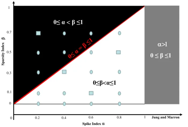
3.1 Consistent areas for PCA and sparse PCA . . . 47

3.2 Performance summary of RSPCA . . . 64

3.3 Demonstration of convergence for growingd . . . 66

3.4 Comparison of PCA, ST and RSPCA . . . 67

3.5 Performance summary of RSPCA . . . 68

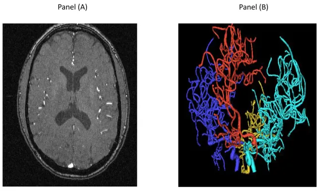
4.1 A single slice MRA image for one person . . . 85

4.2 The binary tree from the back (gold) tree . . . 85

4.3 Equivalence from the flipping indicated by the colored arrows . . . 87

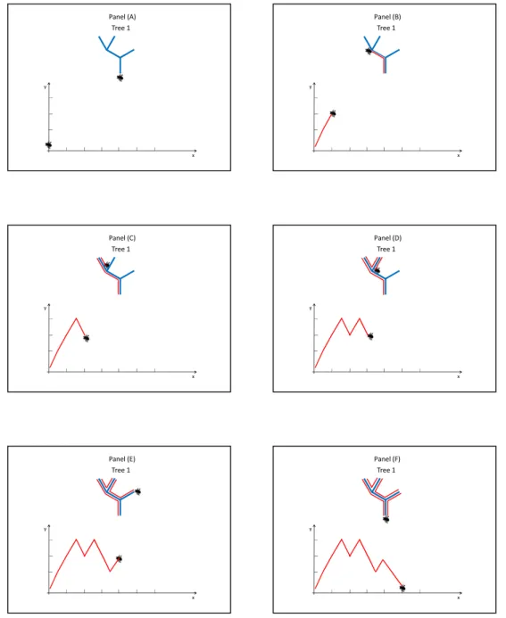
4.4 Dyck path of a tree . . . 89

4.5 The branch length representation . . . 91

4.6 The support tree of individual . . . 93

4.7 Three support individual binary (back) trees . . . 95

4.8 The Dyck path curves of the 98 support binary (back) trees . . . 95

4.9 PCA of the Dyck path curves . . . 97

4.10 Five PC1 projection trees . . . 98

4.11 DiProPerm test on the DWD scores . . . 99

4.12 Five five DWD projection trees . . . 100

4.13 The 35 level pruned (Back) tree . . . 102

4.14 The individual (back) tree under the pruned tree structure. . . 102

4.15 The Dyck paths of the level 35 pruned binary (back) trees . . . 103

4.16 DiProPerm test on the DWD scores . . . 104

(9)

(10)

Chapter 1 Introduction

This thesis contains two major areas. The first one is to study asymptotic properties of Principal Component Analysis (PCA) and sparse PCA. The second one is to apply functional data analysis to tree structured data objects.

High dimensionality has become a common feature of data encountered in many diver-gent fields, such as genomics, economics and finance. This provides modern challenges for statistical analysis. To cope with the high dimensionality, dimension reduction and sparsity constraints become interesting.

(11)

affect PCA consistency.

High Dimension, Low Sample Size (HDLSS) asymptotics are based on the limit as the dimension d → ∞ with the sample size n being fixed. It was originally studied by Casella and Hwang (1982) in the context of James-Stein estimation. Ahn et al. (2007) first studied the HDLSS asymptotic properties of PCA. A comprehensive result of this type is Jung and Marron (2009). As shown in Johnstone and Lu (2009), exploitation of sparsity helps to recover consistency, even in contexts where conventional PCA is inconsistent. In Chapter 3, we study the asymptotic properties of sparse PCA in HDLSS settings, as in Shen et al. (2012a). Under the previously studied spike covariance assumption, we show that sparse PCA is consistent under the same large spike condition that was used to gain insight into for conventional PCA. Under a broad range of small spike conditions, we identify a large, new set of sparsity assumptions where sparse PCA is consistent, but conventional PCA is strongly inconsistent. The boundaries of the consistent region are clarified using an oracle result.

(12)

Chapter 2 A General Framework for Consistency of

PCA

2.1 Introduction

Principal Component Analysis (PCA) is an important visualization and dimension reduction tool which finds orthogonal directions reflecting maximal variation in the data. This allows the low dimensional representation of data, by projecting data onto these directions. PCA is usually obtained by an eigen decomposition of the sample variance-covariance matrix of the data. Properties of the sample eigenvalues and eigenvectors have been analyzed under several domains of asymptotics.

In this thesis, we develop ageneral asymptotic frameworkto explore interesting transitions among the various asymptotic domains. The general framework includes the traditional asymptotic setups as special cases, which allows careful study of the connections among the various setups, and more importantly it investigates scenarios that have not been considered before, and offers new insights into the consistency (in the sense that the angle between estimated and population eigen direction tends to 0, or the inner product tends to 1) and strong-inconsistency(where the angle tends to π₂, i.e., the inner product tends to 0) properties of PCA, along with some technically challenging convergence rates.

Existing asymptotic studies of PCA roughly fall into three domains:

(13)

and the dimensiondis fixed (hence the ratio n_d → ∞). For example, see Girshick (1939); Lawley (1956); Anderson (1963, 1984); Jackson (1991).

(b) The second domain considersrandom matrixtheory, where both the sample sizenand the dimensiond increase to infinity, with the ratio n_d → c, a constant mostly assumed to be within (0,∞). Representative work includes Biehl and Mietzner (1994); Watkin and Nadal (1994); Reimann et al. (1996); Hoyle and Rattray (2003) from the statistical physics literature, as well as Johnstone (2001); Baik et al. (2005); Baik and Silverstein (2006); Onatski (2006); Paul (2007); Nadler (2008); Johnstone and Lu (2009); Lee et al. (2010b); Benaych-Georges and Nadakuditi (2011) from the statistics literature.

(c) The third domain ishigh dimension low sample size (HDLSS)asymptotics, which is based on the limit, as the dimensiond→ ∞, with the sample sizenbeing fixed (hence the ratio n_d → 0). HDLSS asymptotics was originally studied by Casella and Hwang (1982), and recently rediscovered by Hall et al. (2005). PCA has been studied using the HDLSS asymptotics by Ahn et al. (2007); Jung and Marron (2009).

PCA consistency and (strong) inconsistency, defined in terms of angles, are important properties that have been studied before. A common technical device is the spike covariance model, initially introduced by Johnstone (2001). This model has been used in this context by, for example, Nadler (2008); Johnstone and Lu (2009); Jung and Marron (2009). An interesting, more general model has been considered by Benaych-Georges and Nadakuditi (2011).

Under the spike model, the first few eigenvalues are much larger than the others. Amajor point of the present chapteris that there are three critical features whose relationships drive the consistency properties of PCA, namely

(1) the sample information: the sample size n, which has a positive contribution to, i.e. encourages, the consistency of the sample eigenvectors.

(14)

(3) the spike information: the relative sizes of the several leading eigenvalues, which also has a positive contribution to the consistency.

Our general framework considers increasing sample size n, increasing dimension d, and increasing spike information, and clearly characterizes how their relationships determine the consistency and strong-inconsistency regions of PCA, along with the boundary between these two regions. In addition, our theorems demonstrate the transitions among the existing do-mains of asymptotics, and for the first time to the best of our knowledge, enable one to understand the connections among them. Note that the classical domain ((a) above) assumes increasing sample size n while fixing dimension d; the random matrix domain ((b) above) assumes increasing sample sizenand increasing dimension d, while fixing the spike informa-tion; the HDLSS domain ((c) above) fixes the sample size, and increases the dimension and the spike information, and thus are all boundary cases of our general framework.

(A) Single Spike - Example 1.1 (B) Multi Spike - Example 1.2

γ S am p le Ind ex ( Joh n stone an d L u (2009 ))

0≤ α + γ <1 1

1 Spike Index (Jung and Marron (2009)) a

α + γ >1

Consistency Strong Inconsistency

C onsi stenc y S trong I nc onsi stenc y (0,0) S am p le Ind ex

Spike Index (Jung and Marron (2009)) a

0≤ α + γ <1 1

1 α + γ >1, γ >0

Subspace Consistency Strong Inconsistency

(0,0) γ

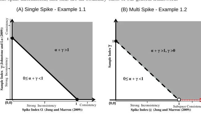
Figure 2.1: General consistency areas for PCA

(15)

existing results. The comparisons and connections are graphically illustrated in Figure 2.1. Here some strong assumptions are made for the purpose of convenient comparison. For these two models, the three types of information and their relationships can be mathematically quantified by two indices, namely thespike indexα and thesample index γ.

Example 2.1.1. (Single-component spike model) Assume thatX1, . . . , Xnare random sample

vectors from a d-dimensional normal distribution N(0,Σ), where the sample size n ∼ dγ

(γ ≥0 is defined as the sample index) and the covariance matrixΣ has the eigenvalues as

λ1 ∼dα, λ2 =· · ·=λd= 1, α≥0,

where the constantα is defined as the spike index.

Our Corollary 2.2.1, applied to this example, shows that the maximal sample eigenvector

is consistent when α+γ >1 (the grey region in Panel (A)), and strongly inconsistent when 0 ≤ α+γ < 1 (the white triangle in Panel (A)). Our Theorem 2.3.1 explored behavior on the diagonal boundaryα+γ = 1. These very general new results connect with many existing ones:

• Previous Results I - the classical domain:

Theorem 1 of Anderson (1963) implied that for fixed dimensiondand finite eigenvalues,

when the sample sizen→ ∞ (i.e. γ → ∞, the limit on the vertical axis), the maximal

sample eigenvector is consistent. This case is the upper left corner of Panel (A) of

Figure 2.1.

• Previous Results II - the random matrix domain:

(a) The results of Johnstone and Lu (2009) appear on the vertical axis in Panel (A)

where the spike index α = 0 (as they fix the spike information): the first sample eigenvector is consistent when the sample index γ > 1 and strongly inconsistent whenγ <1.

(b) Nadler (2008) explored the interesting boundary case of α= 0, γ= 1 (i.e. d_n →c

(16)

on the vertical axis.

• Previous Results III - the HDLSS domain:

(a) The theorems of Jung and Marron (2009) are represented on the horizontal axis in

Panel (A) when the sample indexγ = 0 (as they fix the sample size): the maximal sample eigenvector is consistent with the first population eigenvector when the spike

indexα >1 and strongly inconsistent when α <1.

(b) Jung et al. (2012) deeply explored limiting behavior at the boundaryα= 1, γ= 0. This result appears in Panel (A) as the single solid circle α= 1 on the horizontal axis.

• Our Results hence nicely connect existing domains of asymptotics, and give a much more complete characterization for the regions of PCA consistency, subspace

consis-tency, and strong inconsistency. We also investigate the consistency of the other sample

eigenvectors, and asymptotic properties of all the sample eigenvalues. Furthermore, we

provide a new general connection between Previous Results II (a) and III (b), by doing a

deeper explanation of assumptions on the boundary case -α+γ = 1. We also establish technically challenging convergence rates within each region, which have not been studied

before.

Example 2.1.2. (Multiple-component spike model) Assume that the covariance matrixΣ in Example 2.1.1 has the following eigenvalues

λj = 

  

  

cjdα if j≤m,

1 if j > m,

α≥0,

where m is a finite positive integer, the constants cj, j = 1,· · · , m, are positive and satisfy

thatcj > cj+1>1,j = 1,· · · , m−1.

Our Corollary 2.2.3, when applied to this example, shows that the first m sample

(17)

1, γ >0 (the grey region in Panel (B)), instead of being subspace consistent (Jung and Mar-ron, 2009), and strongly inconsistent whenα+γ < 1, the white triangle in Panel (B). This very general new result connects with many others in the existing literature:

• Previous Results I - the classical domain:

Theorem 1 of Anderson (1963) implied that for fixed dimensiondand finite eigenvalues,

when the sample size n→ ∞ (i.e. γ → ∞, the limit on the vertical axis), the first m

sample eigenvectors are consistent, while the other sample eigenvectors are subspace

consistent. This case is the upper left corner of Panel (B) of Figure 2.1.

• Previous Results II - the random matrix domain:

Paul (2007) explored asymptotic properties of the first m eigenvectors and eigenvalues

in the interesting boundary case of α = 0, γ = 1, i.e., _nd → c with c ∈ (0,1). This result appears in Panel (B) as the solid circle γ = 1 on the vertical axis. Paul and Johnstone (2007a) considered a similar framework but from minimax risk analysis

per-spective. Nadler (2008); Johnstone and Lu (2009) did not study multiple spike models.

• Previous Results III - the HDLSS domain:

The theorems of Jung and Marron (2009) are valid on the horizontal axis in Panel (B)

where the sample index γ = 0. In particular, for this example, their results showed that the first m sample eigenvectors are not separable when the spike indexα > 1 (the horizontal dotted red line segment), instead they are subspace consistent with their

cor-responding population eigenvectors, and are strongly inconsistent when the spike index

α < 1 (the horizontal solid line segment). They and Jung et al. (2012) did not study the asymptotic behavior on the boundary - the single open circle (α= 1, γ = 0) on the horizontal axis.

• Our Resultscover the classical domain, and are stronger than what Jung and Marron

(2009) obtained: the increasing sample size enables us to separate out the first few

lead-ing eigenvectors and characterize individual consistency, while only subspace consistency

(18)

The rest of Chapter 2 is organized as follows. Section 2.1.1 first introduces our nota-tions and several relevant consistency concepts, and then provides intuitive explananota-tions of our eigenvalue assumptions and the corresponding results. Section 2.2 presents the main theoretical results of Chapter 2, stating the asymptotic properties of the sample eigenvalues and eigenvectors under our general framework. Section 2.2.1 first considers the most general cases: multiple spike models with tiered eigenvalues. Sections 2.2.2 and 2.2.3 then discuss the implications and insights learned for single-component and multiple-component spike models (without tiered eigenvalues), respectively. Section 2.3 then investigates the property of PCA on the boundary between consistency and strong inconsistency regions under single spike models. Section 2.5 contains the technical proofs of the main theorems. Section 2.4 presents the some future work that we plan to investigate.

2.1.1 Notation

Let the population covariance matrix be Σ, whose eigen decomposition is

Σ =UΛUT,

where Λ is the diagonal matrix of population eigenvaluesλ1 ≥λ2 ≥. . . ≥λd, and U is the

matrix of corresponding eigenvectorsU = [u1, . . . , ud].

First, we make the following assumption about our sample:

Assumption 2.1.1. X1, . . . , Xn are a random sample from a d-dimensional normal

distri-bution N(0,Σ).

Denote the data matrix by X = [X1, . . . , Xn]d×n and the sample covariance matrix by

ˆ

Σ =n−1XXT. Then, ˆΣ can be similarly decomposed as

ˆ

Σ = ˆUΛ ˆˆUT, (2.1)

where ˆΛ is the diagonal matrix of sample eigenvalues ˆλ1 ≥λˆ2 ≥. . .≥ˆλd and ˆU is the matrix

(19)

Below we introduce asymptotic notations that will be used in our theoretical studies. Assume that{ξn:n= 1, . . . ,∞}is a sequence of random variables, and{an:n= 1, . . . ,∞}

is a sequence of constant values.

• Denoteξn= oa.s(an) if limn→∞_aξn

n = 0 almost surely.

• Denoteξn= Oa.s(an) if limn→∞

ξn

an

≤calmost surely, for some constant c >0. • Denoteξna∼.s an ifc2 ≤limn→∞ξ_an_n ≤ limn→∞_aξn_n ≤c1 almost surely, for two constants

c1≥c2>0.

2.1.2 Concepts

Below we list six important concepts relevant for consistency and strong inconsistency, some of which are modified from the related concepts given by Jung and Marron (2009); Shen et al. (2012a).

Let ¯uj be any sample based estimator of uj for j = 1, . . . , n∧d. For example, ¯uj = ˆuj,

thejth sample eigenvector.

• Consistency: ¯uj is consistent with its population counterpart uj if |< u¯j, uj >|=

1 + oa.s(1), i.e the angle between ¯uj and uj tends to 0.

• Consistency with convergence rate an: ¯uj is consistent with uj with the

conver-gence rateanif|<u¯j, uj >|= 1 + Oa.s(an). For example,an=

nλ1

d 1₂

.

• Strong inconsistency: ¯uj is strongly inconsistent withuj if|<u¯j, uj >|= oa.s(1), i.e

the angle between ¯uj and uj tends to π₂.

• Strong inconsistency with convergence rate an: ¯uj is strongly inconsistent with

the convergence ratean if|<u¯j, uj >|= Oa.s(an).

LetH be an index set, e.g. H={m+ 1,· · ·, d}. Supposej∈H.

• Subspace consistency: ¯uj is subspace consistent withuj if

(20)

where span{uk, k∈H} is the linear span generated by {uk, k∈H}.

• Subspace consistency with convergence ratean: ¯uj,j∈H, is subspace consistent

withuj with convergence rate an if

angle (¯uj,span{uk, k∈H}) = Oa.s(an).

2.1.3 Assumptions

Our main theorems in Section 2.2.1 are very general, but also quite complicated. Insights and connections to previous work come from various special cases, which are carefully studied as corollaries in Sections 2.2.2 and 2.2.3. For these corollaries and main theorems, it is useful to develop a sequence of eigenvalue assumptions of increasing complexity.

Single Component Spike Models

Here we assume the maximal eigenvalue λ1 dominates the other eigenvalues. The other

eigenvalues are assumed to be asymptotically equivalent. For simplicity of notation, we assume they are asymptotically equivalent to 1. More specifically,

Assumption 2.1.2. As n→ ∞, the population eigenvalues satisfy

• λ2

λ1 →0, λ2 ∼ · · · ∼λd∼1.

As discussed in the Introduction, we consider the delicate balance among the positive sample informationn, the positivespike informationλ1, and the negativevariable information

d, and characterize the various PCA consistency and strong-inconsistency regions.

Corollary 2.2.1 suggests that the asymptotic properties of the sample eigenvalues and eigenvectors depend on the relative strength of the positive information and the negative in-formation, as measured by two ratios. First, _nλd

1, corresponding tod

1−(α+γ)_{in Example 2.1.1,}

(21)

The following discussion and the scenarios in Corollary 2.2.1 are arranged according to a decreasing amount of positive information:

• Corollary 2.2.1(a): If the amount of positive information dominates the amount of

negative information up to the maximal eigenvalue, i.e. _nλd

1 → 0, the maximal sample

eigenvector is consistent, and the other sample eigenvectors are subspace consistent.

• Corollary 2.2.1(b): In addition, if the amount of negative information dominates the amount of positive information for the eigenvalues whose indices are greater than 1, i.e.

d

n → ∞, then the corresponding sample eigenvectors are strongly-inconsistent.

• Corollary 2.2.1(c): On the other hand, if the amount of negative information always dominates, i.e. _nλd

1 → ∞, then the sample eigenvalues are asymptotically

indistinguish-able, and the sample eigenvectors are strongly inconsistent.

Corollary 2.2.1 considers the cases where n → ∞. Parallel results can be obtained for the fixed ncases (i.e. the HDLSS domain) as summarized in Corollary 2.2.2. In comparison with Jung and Marron (2009), we make more general assumptions on the population eigen-values, and obtain the corresponding convergence rate results, which were not considered in Jung and Marron (2009).

Under the HDLSS domain, Assumption 2.1.2 on the eigenvalues becomes

Assumption 2.1.3. As d→ ∞, the population eigenvalues satisfy

• λ2

λ1 →0, λ2 ∼ · · · ∼λd∼1.

Multiple Component Spike Models

We now state a parallel series of assumptions for multiple spike models with m dominating spikes where m∈[1, n∧d], and each of the first m eigenvalues is uniquely identifiable.

Assumption 2.1.4. As n→ ∞, the population eigenvalues satisfy

• limn→∞λ_λj

(22)

• λm+1

λm →0,

• λm+1 ∼ · · · ∼λd∼1.

In the same spirit as Corollary 2.2.1, Corollary 2.2.3 states asymptotic properties of the sample eigenvalues and eigenvectors in a trichotomous manner, separated by the size of _nλd

j, which again measures the relative strength of positive and negative information. We arrange the scenarios below and in Corollary 2.2.3 in the order of decreasing amount of positive information:

• Corollary 2.2.3(a): If the amount of positive information dominates the amount of

negative information up to themth spike, i.e. _nλd

m →0, then each of the firstmsample eigenvectors is consistent, and the additional ones are subspace consistent.

• Corollary 2.2.3(b): Otherwise, if the amount of positive information dominates the

amount of negative information only up to thehth spike (h∈[1, m]), i.e. _nλd

h →0 and

d

nλh+1 → ∞, then each of the first h sample eigenvector is consistent, and each of the

remaining higher-order sample eigenvectors is strongly-inconsistent.

• Corollary 2.2.3(c): Finally, if the amount of negative information always dominates, i.e.

d

nλ1 → ∞, then the sample eigenvalues are asymptotically indistinguishable, and the

sample eigenvectors are strongly inconsistent.

Corollary 2.2.3 considers the cases where n→ ∞. Corresponding results can be obtained for the fixed ncases in Corollary 2.2.4. Assumption 2.1.4 then becomes

Assumption 2.1.5. As d→ ∞, the population eigenvalues satisfy

• limd→∞ λ_λj_i = 0, 1≤i < j ≤m+ 1,

(23)

Multiple Component Spike Models with Tiered Eigenvalues

Finally, we consider models where them dominating eigenvalues can be grouped intor tiers. Within tiers, eigenvalues are either of the same limit, or in some cases have the same order.

Below we first consider cases with an increasing sample sizen. To fix ideas, assume that there areqleigenvalues in thelth tier, and the positive integersqlsatisfyPrl=1ql=m. Define

q0 = 0,qr+1=d−Prl=1ql, and the index set of the eigenvalues in thelth tier as

Hl= (_l₋₁

X

k=0

qk+ 1, l−1 X

k=0

qk+ 2,· · · , l−1 X

k=0

qk+ql )

, l= 1,· · · , r+ 1. (2.2)

In addition, we assume the eigenvalues in the lth tier have the same asymptotic behavior, represented in terms of a sequence δl(>0), in the sense that

                

limn→∞λ_δ₁1 = · · · = limn→∞

λq₁

δ1 = 1,

limn→∞λq_δ1+1

2 = · · · = limn→∞

λq₁₊q₂

δ2 = 1,

.. . limn→∞

λq₁₊···_qr₋₁₊₁

δr = · · · = limn→∞

λq1+···+qr

δr = 1.

(2.3)

We impose the following assumption on the eigenvalues:

Assumption 2.1.6. As n → ∞, the population eigenvalues satisfy (2.3) and the following properties:

• limn→∞δ_δj

i <1, 1≤i < j ≤r,

• λm+1

λm →0,

• λm+1 ∼ · · · ∼λd∼1.

Under the above setup, our main Theorem 2.2.1 suggests that the eigenvalues with the same limiting behavior can not be individually estimated consistently; their estimates are either subspace consistent with the linear space spanned by them, or the estimates are strongly inconsistent. Convergence rates depend on the eigenvalue ratios among the tiers, defined as al = max1≤k≤l

δk+1

(24)

Now for the fixed n cases, we assume that as d→ ∞, the first m eigenvalues fall into r tiers according to the following assumption (2.4):



       

       

λ1 ∼ · · · ∼ λq1 ∼ δ1,

λq1+1 ∼ · · · ∼ λq1+q2 ∼ δ2,

.. .

λq1+···qr−1+1 ∼ · · · ∼ λm ∼ δr.

(2.4)

We then make the following eigenvalue assumption:

Assumption 2.1.7. As d→ ∞, the population eigenvalues satisfy (2.4) and the following properties:

• limd→∞ δ_δj_i = 0, 1≤i < j≤r,

• λm+1

λm →0,

• λm+1 ∼ · · · ∼λd∼1.

Different from (2.3) of Theorem 2.2.1, now with a fixed sample sizen, the eigenvalues in the same tier are assumed to be of the same order, rather than of the same limit as assumed when n increases to ∞ (Theorem 2.2.1). Theorem 2.2.2 shows that one can no longer separately estimate the eigenvalues of the same order whennis fixed, which is feasible with an increasing nas long as they do not have the same limit as stated in Theorem 2.2.1.

2.2 Asymptotic Properties of PCA

We state main theorems for multiple-component spike models with tiered eigenvalues in Section 2.2.1, and corollaries for simpler single and multiple spike models in Sections 2.2.2 and 2.2.3, respectively. Technical proofs will be provided in Section 2.5.

2.2.1 Multiple Component Spike Models with Tiered Eigenvalues

(25)

same or have the same limit or are of the same order, and the eigenvalues within different tiers have either different limits or are of different orders. The theorems show that the eigenvalues in the same tier can not be individually estimated consistently.

Theorem 2.2.1. Under Assumptions 2.1.1 and 2.1.6, the results below hold.

(a) If _nδd

r →0, then the sample eigenvalues satisfy

           ˆ λj λj

a.s

−→1, 1≤j≤m,

ˆ λj

a.s

∼ d

n, m+ 1≤j≤[n∧(d−m)],

ˆ

λj = Oa.s d_n

, [n∧(d−m) + 1]≤j≤n∧d;

(2.5)

(There is no need to consider the last scenario above if [n∧(d−m) + 1]> n∧d.) In addition, the sample eigenvectors satisfy



 

 

angle(ˆuj,span{uk, k∈Hl}) = h

oa.s(al)∨Oa.s

d nδl

i1₂

, j∈Hl,1≤l≤r,

angle(ˆuj,span{uk, k∈Hr+1}) = h

oa.s(ar)∨Oa.s

d nδr

i1₂

, m+ 1≤j≤n∧d, (2.6) which shows that the sample eigenvector whose index is in Hl, l ∈ [1, r], is subspace

consistent with the linear space spanned by the population eigenvectors whose labels are

inHl, with convergence rate

al∨_nδd

l

1₂

; each of the rest sample eigenvectors is subspace

consistent with the linear space spanned by Hr+1, with convergence rate

ar∨ _nδd_r 1₂

.

(b) If there exists a constant h, 1 ≤h ≤ r, such that _nδd

h → 0 and

d

nδh+1 → ∞, then the

sample eigenvalues satisfy

     ˆ λj λj

a.s

−→1, j∈Hl,1≤l≤h,

ˆ λj

a.s

∼ d_n, Ph

l=1ql < j≤n∧d;

(26)

in addition, the sample eigenvectors satisfy     

oa.s(al)∨Oa.s

d nδl

i1₂

, j ∈Hl,1≤l≤h, |<uˆj, uj >|2= Oa.s

_nλ

j

d

, Ph

l=1ql< j≤n∧d,

(2.8) which shows that the sample eigenvector whose index is in Hl, 1 ≤l ≤ h, is subspace

consistent with the space spanned by the population eigenvectors whose labels are also in

Hl, with the convergence rate

al∨_nδd_l 1

2

; each of the rest of the sample eigenvectors is

strongly inconsistent, with the convergence rate

_nλ j d 1 2 .

(c) If _nδd

1 → ∞, then the sample eigenvalues satisfy

ˆ λj

a.s

∼ d

n, j= 1,· · ·, n∧d; (2.9)

in addition, the sample eigenvectors satisfy

|<uˆj, uj >|2= Oa.s

nλj

d

, j= 1,· · ·, n∧d, (2.10)

which shows that the sample eigenvector uˆj is strongly inconsistent with uj, with the

convergence rate (nλj

d )

1

2, j= 1,· · ·, n∧d, respectively.

The following comments can be made for the results of Theorem 2.2.1.

• The cases covered by Theorem 2.2.1 were not studied by Paul (2007), which required

the eigenvalues to be individually estimable.

• The asymptotic properties of the sample eigenvectors in Theorem 2.2.1 will not change under more general assumptions on the population eigenvalues. For example, if limn→∞λm+1=

· · ·= limn→∞λd=cwithcbeing a constant, the condition λ_λm_m+1 →0 can be relaxed to

assuming only thatλmis at least a constant away fromλm+1 such that limn→∞λm> c;

in addition, if d_n →0 or∞, the result “ˆλj

a.s

∼ d

n” can be strengthened to “ˆλj

a.s

−→c_nd”.

(27)

and the eigenvalues satisfying (2.3). Then, the results of Theorem 2.2.1(a) are consis-tent with the classical asymptotic subspace consistency results implied by Theorem 1 of Anderson (1963).

The above Theorem 2.2.1 considers the cases wheren→ ∞. We can obtain parallel results for the fixed ncases (i.e. the HDLSS domain) as summarized below in Theorem 2.2.2. Note that we make more general assumptions on the population eigenvalues than Jung and Marron (2009), and obtain the corresponding convergence rate results, which were not considered before.

It is first worth pointing out that withnbeing fixed, we will consider convergence in prob-ability, instead of almost surely. Consequently, we need to modify the convergence notations introduced in Section 2.1.1 to the following:

• Denoteξd= op(ad) if limd→∞_aξd

d = 0 in probability.

• Denote ξd = Op(ad) if limd→∞ ξd ad

≤ z in probability, where the random variable z

satisfies P(0< z <∞) = 1.

• Denote ξd

p

∼ ad if z2 ≤ limd→∞aξdd ≤ limd→∞

ξd

ad ≤ z1 in probability, where the two random variables satisfy P(0< z2≤z1 <∞) = 1.

The consistency concepts in Section 2.1.2 are modified correspondingly.

Theorem 2.2.2. Under Assumptions 2.1.1 and 2.1.7, the results below hold.

(a) If there exists a constant h, 1 ≤ h ≤ r, such that _δd

h → 0 and

d

δh+1 → ∞, then the

sample eigenvalues satisfy

     ˆ λj p

∼λj, j ∈Hl,1≤l≤h, nˆλj

d

p

−→K, Ph

l=1qh< j ≤n, with K= limd→∞d−1Pd_j₌_m₊₁λj;

(2.11)



 

 

Op

al∨ nδdl

i1

2

, j∈Hl,1≤l≤h, |<uˆj, uj >|2= Op

_nλ

j

d

, Ph

l=1qh < j≤n,

(28)

which shows that the sample eigenvector whose index is in Hl, 1 ≤l ≤ h, is subspace

consistent with space spanned by the population eigenvector whose labels are also inHl,

with the convergence rate

al∨_nδd_l 1

2

, l = 1,· · · , h. For Ph

l=1qh < j ≤n, the sample

eigenvector uˆj is strongly inconsistent withuj, with the convergence rate _nλ

j

d 1

2

.

(b) If _δd

1 → ∞, then the sample eigenvalues satisfy

nλˆj

d

p

−

→K, j= 1,· · · , n; (2.13)

|<uˆj, uj >|2= Op

nλj

d

, j= 1,· · · , n, (2.14)

which shows that the sample eigenvector uˆj is strongly inconsistent with uj, with the

convergence rate (nλj

d )

1

2, j= 1,· · ·, n, respectively.

The results of Theorem 2.2.2 suggest that, for the population eigenvalues in each tier (which are of the same order), the corresponding sample eigenvalues can not be separated asymptotically; on the other hand, for the eigenvalues from different tiers, the corresponding sample eigenvalues can be separated asymptotically. Hence, if each tier only has one eigen-value, i.e. r =m andq1=· · ·=qr= 1, the sample eigenvalues are asymptotically separable,

in which case we can strengthen the result “ˆλj

p

∼ λj” in (2.11) to “

ˆ

λj

p

−→ χn2

n”, as stated in

(2.15) of Corollary 2.2.2 and (2.16) of Corollary 2.2.4.

2.2.2 Single Component Spike Models

We now consider special cases of Theorem 2.2.1 withm= 1, which are stated in the following Corollary 2.2.1 for single-component spike models.

Corollary 2.2.1. Under Assumptions 2.1.1 and 2.1.2, the following holds.

(a) If _nλd

(29)

suggests thatuˆ1 is consistent with the convergence rate

d nλ1

1₂

, and forj= 2,· · ·, n∧d,

ˆ

uj is subspace consistent with convergence rate

d nλ1

1₂

.

(b) If _nλd

1 →0 and

d

n → ∞, then it follows from (2.7) that

ˆ λ1

λ1 a.s

−→1; λˆj a∼.s

d

n, 2≤j ≤n∧d,

and (2.8)suggests thatuˆ1 is consistent with convergence rate

d nλ1

1₂

; forj∈[2, n∧d],

ˆ

uj is strongly inconsistent with rate _nλ

j

d 1₂

.

(c) If _nλd

1 → ∞, then (2.9)and (2.10) remain the same: for j= 1,· · ·, n∧d,

ˆ λj

a.s

∼ _nd, and

ˆ

uj is strongly inconsistent with convergence rate (nλ_dj)

1 2.

Having stated the main results for single-component spike models, we now offer several remarks regarding the conditions assumed in Corollary 2.2.1 and the connections with the existing results about PCA consistency.

• In Corollary 2.2.1, the dimensiondcan be fixed. In addition, assume limn→∞λ2 =· · ·=

limn→∞λd=c <limn→∞λ1 <limn→∞λ1 <∞ (for a constantc), which corresponds to

the classical asymptotic framework considered by Anderson (1963). Theorem 1 of An-derson (1963) implies that the maximal sample eigenvector is consistent, and the rest of the sample eigenvectors are subspace consistent with their corresponding eigenvectors, which is consistent with our Corollary 2.2.1(a).

• Assuming fixedλ1 and _nd →cwithcbeing a constant, Nadler (2008); Johnstone and Lu

(2009); Benaych-Georges and Nadakuditi (2011) obtained the results inPrevious Results II - the random matrix domainin Example 2.1.1, which indicate that, as n→ ∞, the maximal sample eigenvector ˆu1 is consistent when d_n → 0, and inconsistent when _nd →

∞. Our Corollary 2.2.1 includes this as a special case. In addition, Corollary 2.2.1 offers more than just relaxing the fixed λ1 assumption: it characterizes how an increasing λ1

(30)

the asymptotic properties of the higher order sample eigenvalues and eigenvectors, all of which have not been investigated before.

• The asymptotic properties of the sample eigenvectors as in Corollary 2.2.1 remain

valid under more general assumptions on the population eigenvalues. For example, if limn→∞λ2 = · · · = limn→∞λd = c with c being a constant, the condition λ_λ2₁ → 0

can be relaxed to assuming only thatλ1 is at least a constant away from λ2 such that

lim_n→∞λ1 > c. Hence, for the models considered by Johnstone and Lu (2009), our

results of the maximal sample eigenvector are the same as theirs. In addition, if _nd →0 or∞, the result “ˆλj

a.s

∼ _nd” in Corollary 2.2.1 can be strengthened to “ˆλj

a.s

−→c_nd”.

Considering the fixed n cases (i.e. the HDLSS domain), Theorem 2.2.2 reduces to the following Corollary 2.2.2 for single spike models.

(a) If _λd

1 →0, then (2.11) is strengthened to

     ˆ λ1 λ1 p

−→ χn2

n,

nλˆj

d

p

−

→K, 2≤j≤n, with K = limd→∞

Pd j=2λj

d ,

(2.15)

and(2.12)suggests thatuˆ1is consistent with convergence rate

d nλ1

1₂

, and forj∈[2, n],

ˆ

uj is strongly inconsistent with convergence rate _nλ

j

d 1₂

.

(b) If _λd

1 → ∞, then (2.13) becomes

nλˆj

d

p

−→ K, for j = 1,· · ·, n, and (2.14) suggests that

ˆ

1 2.

Note that in (2.15): ifn→ ∞, then we have χn2

n

a.s

−→1. This is consistent with the results

in (a) and (b) of Corollary 2.2.1, where λˆ1

λ1 a.s

−→1.

2.2.3 Multiple Component Spike Models

(31)

q1 =· · ·=qr = 1, i.e. each of them tiers only contains one eigenvalue.

(a) If _nλd

m →0, then (2.5)remains valid for the sample eigenvalues. (2.6)then suggests that ˆ

uj,j∈[1, m], is consistent with convergence rate

aj∨_nλd_j 1₂

, anduˆj,j∈[m+1, n∧d],

is subspace consistent with convergence rateam∨_nλd_m 1₂

.

(b) If there exists a constant h, 1≤h≤m, such that _nλd

h →0 and

d

nλh+1 → ∞, then (2.7)

becomes

ˆ λj

λj

a.s

−→1, 1≤j≤h; ˆλj

a.s

∼ d

n, h+ 1≤j ≤n∧d,

and (2.8) suggests that uˆj, j ∈ [1, h], is consistent with convergence rate

aj ∨_nλd_j 1₂

,

anduˆj, j∈[h+ 1, n∧d], is strongly inconsistent with convergence rate _nλ

j

d 1₂

.

(c) If _nλd

1 → ∞, then (2.9)and (2.10) remain the same: for j= 1,· · ·, n∧d,

ˆ λj

a.s

∼ d n, and

ˆ

1 2.

We now discuss the conditions needed in the corollary and how the results connect with existing results in the literature.

• In Corollary 2.2.3, the dimensiondcan be fixed. In addition, consider limn→∞λm+1 =

· · · = limn→∞λd = c < limn→∞λm < limn→∞λ1 < ∞. Then, Corollary 2.2.3(a) is

consistent with the classical results implied by Theorem 1 of Anderson (1963).

• Considering fixed λ1,· · · , λm and _nd → c, where c ∈ (0,1), Paul (2007) obtained the

results inPrevious Results II - the random matrix domainin Example 2.1.2. As one can see, our Corollary 2.2.3 relaxes the assumptions of _nd →c∈(0,1) and that λ1,· · ·, λm

are fixed. In addition, we characterize how increasingλ1,· · · , λminteract with the ratio d

n along with the corresponding convergence rates, and study the asymptotic properties

(32)

• The asymptotic properties of the sample eigenvectors in Corollary 2.2.3 will not change

under more general assumptions on the population eigenvalues, as discussed after The-orem 2.2.1.

Corollary 2.2.4 below considers fixed n, and follows from Theorem 2.2.2.

(a) If there exists a constant h, 1≤h≤m, such that _λd

h →0 and

d

λh+1 → ∞, then (2.11)

is strengthened to



 

 

ˆ

λj

p

−→ χ2n

n, 1≤j≤h, nλˆj

d

p

−→K, h+ 1≤j≤n.

(2.16)

(2.12)then suggests that uˆj,j∈[1, h], is consistent with convergence rate

aj ∨_nλd_j 1₂

,

anduˆj, j∈[h+ 1, n], is strongly inconsistent with convergence rate _nλ

j

d 1₂

.

(b) If _λd

1 → ∞, then (2.13) and (2.14)remain valid: for j= 1,· · ·, n,

nˆλj

d

p

−→K, and uˆj is

strongly inconsistent with convergence rate (nλj

d )

1 2.

We remark that in (2.16), ifn→ ∞, then we have χn2

n

a.s

−→1. This is consistent with the result λˆj

λj

a.s

−→1,j∈[1, h], in (a) and (b) of Corollary 2.2.3.

2.3 Balanced Positive and Negative Information

(33)

Theorem 2.3.1. In addition to Assumption 2.1.1, we also assume that as n → ∞, the

population eigenvalues have the following properties:

• λ2

λ1 →0,

• λj →cλ, j = 2,· · · , d, for a constantcλ.

If _nλd

1 →c∈(0,∞), then the sample eigenvalues satisfy



 

 

ˆ

λ1

λ1 a.s

−→1 +ccλ, n

dλˆj

a.s

−→cλ, 2≤j≤n∧d;

(2.17)



 

 

|<uˆ1, u1 >|2= ₁₊1_cc_λ + oa.s(1),

|<uˆj, uj >|2= Oa.s(n_d), 2≤j≤n∧d,

(2.18)

which shows that the limiting angle between the maximal sample eigenvector uˆ1 and u1 is

between 0 and π₂, and each of the additional sample eigenvector uˆj is strongly inconsistent

withuj, with the convergence rate n_d 1

2_.

Below we comment on the results of Theorem 2.3.1.

• Theorems 2.2.1 and 2.3.1 together completely characterizes the phase transition behav-ior of the maximal sample eigenvector ˆu1as _nλd₁ converges to a different limit: asn→ ∞,

ˆ

u1 starts from being consistent when _nλd₁ → 0, to being in-between consistency and

strong inconsistency (with the limiting angle between 0 and π₂) when _nλd

1 →c∈(0,∞),

and finally to being strongly inconsistent when _nλd

1 → ∞.

• The results nicely complement existing results of Nadler (2008); Jung et al. (2012): Nadler

(2008) considered cases with a constantλ1 and _nd →c∈(0,∞) asn→ ∞, and derived

the absolute inner product between ˆu1and u1; Jung et al. (2012) studied scenarios with

fixedn and _λd

1 →c∈(0,∞) as d→ ∞, and showed that the absolute inner product is

(34)

In the context of the illustrating Example 2.1.1, the results of Nadler (2008) correspond to the point on the horizontal axis withα= 0 andγ = 1; the results of Jung et al. (2012) are for the point on the vertical axis withα = 1 and γ = 0; finally, our results are for the solid line withα+γ = 1, which separates the consistency and strong-inconsistency regions.

2.4 Future Work

There are several interesting problems that we will explore in the future. One is to extend our theorems to more general distributions. Another is to build the similar framework to study the asymptotic properties of functional PCA (Dauxois et al., 1982; Bosq, 2000; Hall and Hosseini-Nasab, 2006).

2.5 Proofs

In this section we provide technical proofs for the theorems and corollaries stated in Sec-tion 2.2. The theorems fall into two groups: (1) Theorems 2.2.1, 2.3.1, and Corollar-ies 2.2.1, 2.2.3 consider increasing sample size; (2) Theorem 2.2.2, and CorollarCorollar-ies 2.2.2, 2.2.4 consider the HDLSS settings where the sample size is fixed. Hence we only prove Theo-rems 2.2.1 and 2.3.1 in details below, and point out how the proof can be adjusted to prove Theorem 2.2.2.

(35)

2.5.1 Invariance Property of the Angle

e

1

e

2

u

1

u

2

(A)

(B)

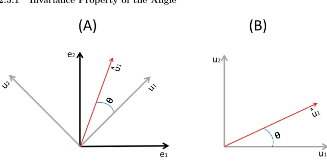
Figure 2.2: Independent between the angle and the basis choice

We note that the angle between the sample eigenvector and its population counterpart doesn’t depend on the specific choice of the basis for thed-dimensional space. Because of this independence, we will choose the population eigenvectorsui,i= 1, . . . , d, as the basis of the

d-dimensional space. Under this basis, the population covariance matrix of Xi,i= 1, . . . , n,

can be written as the following diagonal matrix:

Σ = Λ =



    

λ1 · · · 0

..

. . .. ... 0 · · · λd



    

. (2.19)

This will simplify our mathematical analysis. Equivalently, without loss of generality, for the rest of the chapter, we assume thatXi,i= 1, . . . , n,has thed-dimensional normal distribution

with zero mean and the diagonal covariance matrix as in (2.19).

Now we use a toy example in Figure 2.2 to illustrate this invariance property of the angle. Assume that Xi has a 2-dimensional normal distribution with two eigenvectors u1 and u2,

which are plotted in Panel (A) of Figure 2.2 under a specific basis set of e1 and e2. The θ

(36)

the 2-dimensional space, the angle between ˆu1 and u1 remains the same, as shown in Panel

(B) of Figure 2.2.

2.5.2 Lemmas

The following two lemmas are needed to prove the theorems. The first one is about the asymptotic properties of the largest and smallest eigenvalues of the Wishart distribution, seen in Geman (1980); Silverstein (1985). The second one is the Wielandt’s Inequality (Rao, 2002), which can be used to study asymptotic properties of eigenvalues of a random matrix.

Lemma 2.5.1. Assume that B = 1_sVsVsT, where Vs is an m×s random matrix composed

of iid standard normal random variables. As s → ∞ and m_s → c ∈ [0,∞), the largest and smallest non-zero eigenvalues of B, denoted as λ1(B) and λm∧s(B), converge almost surely

to(1 +√c)2 and (1−√c)2, respectively.

Remark: The results in the thesis cited are for c∈(0,∞), which can be easily extended to include the case of c = 0 by simple coupling arguments, as in (38) of Johnstone and Lu (2009).

Lemma 2.5.2. (Wielandt’s Inequality). If A, B are m×m real real symmetric matrices,

then for all k= 1, . . . , m,

                

λk(A) + λm(B)

λk+1(A) + λm−1(B)

.. .

λm(A) + λk(B)                 

≤λk(A+B)≤                 

λk(A) + λ1(B)

λk−1(A) + λ2(B)

.. .

λ1(A) + λk(B)                  .

2.5.3 Intuitive ideas

(37)

To fix ideas, define Zi = Λ−

1

2X_i for i = 1, . . . , n. Then, the Z_is are iid standard d

-dimensional normal distribution. Denote the jth entry of Zi as zi,j for j = 1, . . . , d. For a

fixedj, define

e

Zj = (z1,j,· · · , zn,j)T, (2.20)

which are iid standardn-dimensional normal distribution.

Note that the dual matrix of the sample covariance matrix can be expressed as

ˆ

ΣD =n−1XTX=

1 n

d X

j=1

λjZe_jZe_jT,

which has the same non-zero eigenvalues as the sample covariance matrix. Hence, we can study the asymptotic properties of the sample eigenvalues through the dual matrix, which we elaborate on below.

Single Component Spike Models

For simplicity, we start with single component spike models, and WLOG, assume that the eigenvalues satisfyλ1 > λ2 =· · ·=λd= 1. Then, the dual matrix can be rewritten as

ˆ ΣD =

λ1

nZe1Ze

T

1 +

1 n

d X

j=2 e

ZjZe_jT.

Denote the two summands in the above expression as Aand B, respectively.

To understand the asymptotic properties of the sample eigenvectors, we first need to understand the asymptotic properties of the sample eigenvalues. For that purpose, we first note that the rank of the matrixAis 1, which suggests thatAhas only one non-zero eigenvalue, denoted as λ1(A) = n−1λ1Ze₁TZe₁. Furthermore, note that the matrix nB has the Wishart

(38)

Two ratios, _nλd

1 and

d

n, play crucial roles in the consistency of the sample eigenvectors.

First, the ratio _nλd

1 affects which one of the matrices A and B plays a dominating role in

determining the maximal eigenvalue ˆλ1 of ˆΣD, which then affects the consistency of the

maximal sample eigenvector ˆu1: if _nλd₁ → 0, ˆλ1 is determined by the matrix A and can be

clearly separated from the other sample eigenvalues, which leads to the consistency of ˆu1; if

d

nλ1 → ∞, ˆλ1 is determined by the matrixB and can not be clearly separated from the other

sample eigenvalues, which makes ˆu1 strongly inconsistent; if _nλd₁ →c∈(0,∞), then it is not

clear which one matrix is dominating, and ˆu1 is neither consistent nor strong inconsistent.

In addition, the ratio _nd determines the consistency of the other sample eigenvectors: If _nd → 0, they are subspace consistent with the subspace spanned by the corresponding population eigenvectors ui,i≥2; If d_n → ∞, then they are strongly inconsistent.

Multiple Component Spike Models

We now discuss the general ideas behind the proof for multiple component spike models. For simplicity, we assume that the first m eigenvalues can be grouped into two tiers, such that λ1 =· · ·=λq=δ1 λq+1 =· · ·=λm =δ2 λm+1 =· · ·=λd= 1. Then, the dual matrix

can be written as

ˆ ΣD =

1 n

q X

j=1

δ1Ze_jZe_jT +

1 n

m X

j=q+1

δ2Ze_jZe_jT +

1 n

d X

j=m+1 e

ZjZe_jT.

We denote the sum of the first two matrices in the above decomposition asA, and the third matrix asB.

Using similar arguments to those in Section 2.5.3, the consistency properties of the sample eigenvectors will depend on three ratios, _nδd

1,

d nδ2 and

d

n, in the following manner:

• The ratio _nδd

1 determines the consistency of the sample eigenvectors in the first tier: If

d

nδ1 →0, the firstq sample eigenvalues can be clearly separated from the other sample

eigenvalues, which results in the subspace consistency of the corresponding sample vec-tors; If _nδd

1 → ∞, these sample eigenvalues can not be clearly separated from the others,

(39)

• The ratio _nδd

2 determines the consistency of the eigenvectors in the second tier: If

d

nδ2 → 0, the sample eigenvalues in the second tier are separable from the others,

and the corresponding sample eigenvectors are subspace consistent; If _nδd

2 → ∞, the

sample eigenvalues in the second tier are separable from the others, which makes the corresponding sample eigenvectors strongly inconsistent.

• Finally, the ratio _nd determines the consistency of the other sample eigenvectors: If

d

n →0, the other sample eigenvectors are subspace consistent with the subspace spanned

by the ui,i≥m+ 1; If _nd → ∞, they are strongly inconsistent.

Different combinations of the limits of the three ratios will give us the various scenarios considered in Theorem 2.2.1.

2.5.4 Asymptotic Properties of the Sample Eigenvalues

We are now in a position to formally prove Theorem 2.2.1. In this section, we first derive the asymptotic properties of the sample eigenvalues, which will be used in studying the consistency of the sample eigenvectors in Section 2.5.5.

We consider general cases where the first m eigenvalues can be grouped intor tiers, and WLOG assume that λ1 = · · · = λq1 = δ1, · · ·, λPr−1

k=0qk+1 = · · · = λm = δr where q0 = 0 and qk are positive integers for k ≥ 1. In addition, we assume that each ratio δj/δi, where

1≤i < j ≤r, converges to a constant less than 1 as n→ ∞. (The following arguments can be extended to cases where only the upper limits of the ratios exist as stated in the theorems, through taking a converging subsequence of the diverging sequence ofn.)

Now we will show the asymptotic properties of the sample eigenvalues as stated in The-orem 2.2.1. For that end, we first note that the dual matrix can be rewritten as the sum of two matrices as follows

ˆ

ΣD =A+B, with A=

1 n

m X

j=1

λjZe_jZe_jT, B =

1 n

d X

j=m+1

λjZe_jZe_jT, (2.21)

(40)

We then establish the asymptotic properties of the eigenvalues ofAand B below in Lem-mas 2.5.3 and 2.5.4, respectively. Finally, the asymptotic properties of the sample eigenvalues of Σ, which are the same as the eigenvalues of the dual matrix, naturally follow (Section 2.5.4).

Asymptotic Properties of the Eigenvalues of the Matrix A

Lemma 2.5.3. As n→ ∞, the eigenvalues of the matrix A in (2.21) satistfy

λk(A)

λk

a.s

−→1, for k= 1,· · ·, m. (2.22)

Proof. We first construct the dual matrixA∗ of the matrixA. Fori= 1,· · · , n, letX_i∗ be the m-dimensional random vector formed by the firstmentries ofXi, i.e. Xi∗ = (Im,0m×(d−m))Xi.

Then,X_i∗ is normal with mean zero and the following covariance matrix Σ∗:

Σ∗= Λ∗ =

      λ− 1 2

1 · · · 0

..

. . .. ... 0 · · · λ−

1 2 m       .

Defined the sample covariance matrix ofX_i∗ as

A∗ = 1 n

m X

j=1

X_i∗(X_i∗)T

= λ1       1 n Pn

i=1zi,21 · · · (λλm1) 1

2 1

n Pn

i=1zi,1zi,m

..

. . .. ...

(λm

λ1) 1

2 1

n Pn

i=1zi,1zi,m · · · λ_λm₁ _n1 Pn

i=1zi,m2       , (2.23)

where thezi,j’s are defined in (2.20) and are iid standard normal random variables.

(41)

The iid properties of thezi,j’s suggest that 1 n n X i=1

zi,kzi,l

a.s

−→     

1 1≤k=l≤m 0 1≤k6=l≤m

, as n→ ∞,

which can be combined with (2.23) to suggest that

1 λ1

A∗−→a.s      

1 · · · 0 ..

. . .. ... 0 · · · bm

     

, as n→ ∞,

wherebk= limn→∞λ_λk

1 ≤1,k= 1,· · · , m. It then follows that

λ1(A)

λ1

= λ1(A

∗₎

λ1 a.s

−→1, as n→ ∞.

Similarly, for k= 2,· · · , m, we have that

λ1(_n1 Pmj=kλjZe_jZe_jT)

λk

a.s

−→1, as n→ ∞. (2.24)

Next we try to derive upper and lower bounds for λk(A). First, Lemma 2.5.2 suggests

that, fork≥2,

λk(A) =λk(

1 n

m X

j=1

λjZe_jZe_jT)≤λ₁(

1 n

m X

j=k

λjZe_jZe_jT) +λ_k(

1 n

k−1 X

j=1

λjZe_jZe_jT). (2.25)

Since the rank of _n1Pk−1

j=1λjZe_jZe_jT is at mostk−1, then it follows that

λk(

1 n

k−1 X

j=1

λjZe_jZe_jT) = 0,

which can be combined with (2.24) to show that

λk(A)

λk

(42)

Now for the lower bound, the expression (5.9) in Jung and Marron (2009) suggests that

λ1(

λk

nZekZe

T

k) +λn(

1 n

m X

j=k+1

λjZe_jZe_jT)≤λ_k(A). (2.27)

Given that the rank of _n1Pm

j=k+1λjZe_jZe_jT is at most m withm < n, then we know that

λn(

1 n

m X

j=k+1

λjZe_jZe_jT) = 0, (2.28)

which, together with (2.27), suggests that asn→ ∞,

λk(A)

λk

≥ 1

λk

λ1(

λk

n ZekZe

T

k). (2.29)

In addition, note that asn→ ∞,

1 λk

λ1(

λk

n ZekZe

T k) =

1 nZe

T kZe_k

a.s

−→1, (2.30)

which, together with (2.29), gives that

λk(A)

λk

≥1, as n→ ∞. (2.31)

The combination of (2.26) and (2.31) suggests (2.22).

Asymptotic Properties of the Eigenvalues of B

Lemma 2.5.4. As n→ ∞, the eigenvalues of the matrix B as defined in (2.21) satisfy

λk(B)

a.s

∼ d

n, k= 1,· · ·, n∧(d−m), (2.32)

Proof. We start with assuming that λm+1 =· · ·=λd= 1. WLOG, we assume that _nd has a

(43)

limit.) Furthermore, we assume that _nd →c≤1. (If c >1, we can consider the dual matrix ofB, whose dimension is (d−m)-by-(d−m), and study its eigenvalues.)

Define V = [Zem+1,Zem+2,· · · ,Ze_d], whose dimension is n-by-(d−m). It then follows that

B = 1_nV VT = d−_nm(_d₋1_mV VT).

Lemma 2.5.1 suggests that λ1(_d₋1_mV VT) a.s

λn∧(d−m)(d−1mV VT)

a.s

∼ 1. It follows that

λk(B) =

d−m n λk(

1 d−mV V

T₎a.s

∼ d

n, k= 1,· · · , n∧(d−m), asn→ ∞,

which then yields (2.32).

The above arguments remain valid for cases whereλm+1 ∼λd∼1.

Asymptotic Properties of the Sample Eigenvalues

We now study the asymptotic properties of the sample eigenvalues ˆλj, for j = 1,· · ·, n∧d,

which are the same as the eigenvalues of the dual matrix ˆΣD, denoted asλj( ˆΣD) =λj(A+B).

According to Lemma 2.5.2, we have that

λj(A) +λn(B)≤λˆj ≤λj(A) +λ1(B),

which suggests

1 λj

λj(A) +

1 λj

λn(B)≤

ˆ λj

λj

≤ 1

λj

λj(A) +

1 λj

λ1(B). (2.33)

In addition, note that Lemma 2.5.4 shows that _λ1

jλn(B) ≤

1

λjλn∧(d−m)(B)

a.s

∼ d

λjn and

1

λjλ1(B)

a.s

∼ d

λjn. Below we consider three scenarios separately. First, if there exists h∈[1, r] such that _nδd

h →0, then

d

nλj →0, for j ∈Hl,l= 1,· · · , h, whereHl is the index set of the eigenvalues in thelth tier. Thus, we have

1 λj

λn(B)

a.s

−→0, and 1 λj

λ1(B) a.s

(44)

The above (2.34), together with (2.33) and Lemma 2.5.3, leads to

ˆ λj

λj

a.s

−→1, j ∈Hl, l= 1,· · · , h. (2.35)

Secondly, if _nδd

h → ∞, then we have d n and n∧(d−m) = n. For j ∈ Hl, l ≥ h, Lemma 2.5.2 suggests that

n

dλj(A) + n

dλn(B)≤ n d ˆ λj ≤

n

dλj(A) + n

dλ1(B). (2.36)

Lemma 2.5.3, together with the condition _nδd

h → ∞, suggests that

n dλj(A)

a.s

−→0 for j ∈Hl

and l ≥h. Using Lemma 2.5.4, we have that n_dλn−m(B) a∼.s1 and n_dλ1(B) a∼.s1. The above,

combined with (2.36), suggests that

ˆ λj

a.s

∼ d

n,

h−1 X

l=1

ql< j ≤n∧d, a.s. (2.37)

Finally, if _nδd

r →0, (2.34) suggests that

ˆ

λj

a.s

−→1, 1≤ j ≤m. In addition, Lemma 2.5.2

suggests that

n

dλj+n−n∧(d−m)(A) + n

dλn∧(d−m)(B)≤ n d ˆ λj ≤

n

dλj(A) + n

dλ1(B). (2.38)

Note that rank ofAis less than or equal tomand it means that forj > m,λj+n−n∧(d−m)(A) =

λj(A) = 0. Furthermore, from Lemma 2.5.4, we have that n_dλ1(B) a∼.s n_dλn∧(d−m)(B) a.s

∼ 1.

Combining above with (2.38), we have ˆλj a∼.s _nd,m+ 1≤j≤n∧(d−m). For j ∈[n∧(d−

m) + 1≤j ≤n∧d], given that ˆλj ≤λˆn∧(d−m), it follows that ˆλj = Oa.s(_nd).

The above arguments can be summarized as follow: if _nδd r →0,

           ˆ λj λj

a.s

−→1, 1≤j≤m

ˆ λj

a.s

∼ _nd, m+ 1≤j ≤n∧d−m ˆ

λj = Oa.s(d_n), n∧(d−m) + 1≤j≤n∧d

. (2.39)

(45)

Combining (2.35), (2.37), and (2.39), we can get the corresponding results (2.5), (2.7), and (2.9) in Theorem 2.2.1.

2.5.5 Asymptotic Properties of the Sample Eigenvectors

We are now ready to derive the asymptotic properties of the sample eigenvectors

ˆ

uj = (ˆu1,j,· · · ,uˆd,j)T, j= 1,· · · , n∧d.

First, we state two results that simplify the proof. As discussed in Section 2.5.1, we choose the population eigevectorsuj (j = 1,· · · , d) as the basis of the d-dimensional space; it then

follows thatuj =ej where the j-th component ofej equals to 1 and all the other components

equal to zero. This yields that

|<uˆj, uj >|2=|<uˆj, ej >|2= ˆu2j,j, (2.40)

and for any index setH,

cos [angle(ˆuj,span{uk, k∈H})] = X

k∈H

ˆ

u2_k,j. (2.41)

Define

ˆ

Ui,j = (ˆuk,l)k∈Hi,l∈Hj, 1≤i, j≤r+ 1, (2.42)

where Hi is defined in (2.2), i= 1,· · ·, r+ 1. Then, the sample eigenvectors matrix can be

rewrote as following.

ˆ

U = [ˆu1,uˆ2,· · · ,uˆd] = 

       

ˆ

U1,1 Uˆ1,2 · · · Uˆ1,r+1

ˆ

U2,1 Uˆ2,2 · · · Uˆ2,r+1

..

. ... ...

ˆ

Ur+1,1 Uˆr+1,2 · · · Uˆr+1,r+1 

       

(46)

Scenario (b) in Theorem 2.2.1

Now consider the scenario (b) in Theorem 2.2.1 in that there exists a constanth∈[1, r], such that _nδd

h →0 and

d

nδh+1 → ∞. Define al = max1≤k≤l

δk+1

δk ,l= 1,· · · , r. From (2.41), in order to show subspace consistent with the convergence rate

al∨ _nδd

l

1₂

in (2.7), we just need to show

X

k∈Hl ˆ

u2_k,j = 1 + oa.s(al)∧Oa.s(

d nδl

), j∈Hl, l= 1,· · ·, h. (2.44)

The following proof is just to show (2.44) forl = 1. For l = 2,· · ·, h, the process is similar and we skip it to avoid the repetition.

Note that for l = 1, the left part of equation (2.44) is just the sum of square column elements of matrix ˆU1,1, where ˆU1,1 is defined (2.42). Thus, in order to show (2.44) for l= 1,

we just need to show that the sum of square column elements of matrix ˆU1,1 converges to 1

with the convergence rate a1∨ _nδd₁. The following proof contains two steps: the first one is

to show sum of square column elements of matrix ˆU1,1 converges to 1; the second step is to

show the convergence rate a1∨_nδd₁.

Now, we will show that the sum of square column entries of the matrix ˆU1,1 converges

to 1. Let Z = (Z1,· · · , Zn), where Zi = Λ−

1

2X_i as defined in Section 2.5.3. Denote S =

(sk,l)d×d= Λ−

1 2UˆΛˆ

1

2 where ˆU is the sample eigevector matrix and ˆΛ is the sample eigenvalue

matrix defined in (2.1), the eigendecomposition of the sample variance matrix ˆΣ. We can show that

SST = 1 nZZ

T_.

Considering the k-th diagonal entry of the matrices on the two sides and noting that sk,j =

λ−

1 2

k λˆ

1 2

juˆk,j, we have the following

1 n

n X

i=1

z_i,k2 =

d X

j=1

s2_k,j =λ−1_k

d X

j=1

ˆ

λjuˆ2k,j, k= 1,· · · , d. (2.45)

As shown earlier, _n1 Pn i=1zi,k2

a.s

−→1, which suggests that ˆu2_k,j ≤ λk

ˆ

λj asn

Shen_unc_0153D_12982.pdf

Sparse PCA Asymptotics and Analysis of Tree Data

Table of Contents

List of Figures

Chapter 1

Introduction

Chapter 2

A General Framework for Consistency of

PCA

2.1

Introduction

2.2

Asymptotic Properties of PCA

2.3

Balanced Positive and Negative Information

2.4

Future Work

2.5

Proofs

e

e

u

u

(A)

(B)