Santiago Casas1, Martin Kunz2, Matteo Martinelli1,3, Valeria Pettorino1,4 1 Institut fuer Theoretische Physik, Universitaet Heidelberg,
Philosophenweg 16, D-69120 Heidelberg, Germany. 2
Département de Physique Théorique and Center for Astroparticle Physics, Université de Genève, 24 quai Ansermet, CH–1211 Genève 4, Switzerland. 3
Institute Lorentz, Leiden University, PO Box 9506, Leiden 2300 RA, The Netherlands, 4
Laboratoire AIM, UMR CEA-CNRS-Paris 7, Irfu,
Service d’Astrophysique CEA Saclay, F-91191 Gif-sur-Yvette, France
Modified Gravity theories generally affect the Poisson equation and the gravitational slip (effective anisotropic stress) in an observable way, that can be parameterized by two generic functions (ηand
µ) of time and space. We bin the time dependence of these functions in redshift and present forecasts on each bin for future surveys like Euclid. We consider both Galaxy Clustering and Weak Lensing surveys, showing the impact of the non-linear regime, treated with two different semi-analytical approximations. In addition to these future observables, we use a prior covariance matrix derived from thePlanckobservations of the Cosmic Microwave Background. Our results show thatηandµ
in different redshift bins are significantly correlated, but including non-linear scales reduces or even eliminates the correlation, breaking the degeneracy between Modified Gravity parameters and the overall amplitude of the matter power spectrum. We further decorrelate parameters with a Zero-phase Component Analysis and identify which combinations of the Modified Gravity parameter amplitudes, in different redshift bins, are best constrained by future surveys. We also extend the analysis to two particular parameterizations of the time evolution of µ and η and consider, in addition to Euclid, also SKA1, SKA2, DESI: we find in this case that future surveys will be able to constrain the current values ofηandµat the 2-5% level when using only linear scales (wavevector k < 0.15 h/Mpc), depending on the specific time parameterization; sensitivity improves to about
1%when non-linearities are included.
CONTENTS
I Introduction . . . 2
II Parameterizing Modified Gravity . . . 3
A Parameterizing gravitational potentials in discrete redshift bins . . . 3
B Parameterizing gravitational potentials with simple smooth functions of the scale factor . . . 4
III The power spectrum in Modified Gravity . . . 6
A The linear power spectrum . . . 6
B Non-linear power spectra. . . 6
1 Halofit . . . 6
2 Prescription for mildly non-linear scales including screening . . . 7
IV Fisher Matrix forecasts . . . 8
A Future large scale galaxy redshift surveys . . . 9
B Galaxy Clustering . . . 9
C Weak Lensing . . . 10
D Covariance and correlation matrix and the Figure of Merit . . . 11
E CMBPlanckpriors . . . 12
V Results: Euclid forecasts for redshift binned parameters . . . 13
A Euclid Galaxy Clustering Survey . . . 13
B Euclid Weak Lensing Survey . . . 15
C Combining Euclid Galaxy Clustering and Weak Lensing, withPlanckdata . . . 16
D Decorrelation of covariance matrices and the Zero-phase Component Analysis. . . 16
1 ZCA for Galaxy Clustering . . . 17
2 ZCA for Weak Lensing . . . 20
3 ZCA for Weak Lensing + Galaxy Clustering + CMBPlanckpriors . . . 21
VI Modified gravity with simple smooth functions of the scale factor . . . 22
A Modified Gravity in the late-time parameterization . . . 23
1 Galaxy Clustering in the linear and mildly non-linear regime . . . 23
2 Weak Lensing in the linear and mildly non-linear regime . . . 24
3 Combining Weak Lensing and Galaxy Clustering . . . 25
4 Forecasts in Modified Gravity for SKA1, SKA2 and DESI . . . 26
B Modified Gravity in the early-time parameterization . . . 27
1 Galaxy Clustering, Weak Lensing and its combination . . . 27
2 Other Surveys: DESI-ELG, SKA1 and SKA2 . . . 31
C Testing the effect of the Hu-Sawicki non-linear prescription on parameter estimation . . . 31
VII Conclusions . . . 34
Acknowledgments . . . 35
References . . . 35
A Transformation of primary variables in Modified Gravity . . . 39
1 Late time parameterization . . . 39
2 Early time parameterization . . . 39
B Derivatives of the Power Spectrum with respect toµandη. . . 40
C Other Decorrelation Methods . . . 41
a Principal Component Analysis . . . 41
b Cholesky decomposition . . . 41
D Weight matrices coefficients . . . 42
E The Kullback-Leibler divergence . . . 44
I. INTRODUCTION
Future large scale structure surveys will be able to measure with percent precision the parameters governing the evolution of matter perturbations. While we have the tools to investigate the standard model, the next challenge is to be able to compare those data with cosmologies that go beyond General Relativity, in order to test whether a fluid component like Dark Energy or similarly a Modified Gravity scenario can better fit the data. On the theoretical side, while many Modified Gravity models are still allowed by type Ia supernova (SNIa) and Cosmic Microwave Background (CMB) data [1]; structure formation can help us to distinguish among them and the standard scenario, thanks to their signatures on the matter power spectrum, in the linear and mildly non-linear regimes (for some examples of forecasts, see [2–4]).
The evolution of matter perturbations can be fully described by two generic functions of time and space [5, 6], which can be measured via Galaxy Clustering and Weak Lensing surveys. In this work we want to forecast how well we can measure those functions, in different redshift bins.
While any two independent functions of the gravitational potentials would do, we follow the notation of [1] and considerµandη: the first modifies the Poisson equation forΨwhile the second is equal to the ratio of the gravitational potentials (and is therefore also a direct observable [6]). We will consider forecasts for the planned surveys Euclid, SKA1 and SKA2 and a subset of DESI, DESI-ELG, using as priors the constraints from recentPlanckdata (see also [7–11] for previous works that address forecasts in Modified Gravity.
In sectionII we defineµand η and parameterize them in three different ways. First, in a general manner, we let these functions vary freely in different redshift bins. Complementarily, we also consider two specific parameterizations of the time evolution proposed in [1]. Here, we also specify the fiducial values of our cosmology for each of the parameterizations considered. SectionIIIdiscusses our treatment for the linear and mildly non-linear regime. Linear spectra are obtained from a modified Boltzmann code [12]; the mild non-linear regime (up to k∼0.5 h/Mpc) compares
II. PARAMETERIZING MODIFIED GRAVITY
In linear perturbation theory, scalar, vector and tensor perturbations do not mix, which allows us to consider only the scalar perturbations in this paper. We work in the conformal Newtonian gauge, with the line element given by
ds2=−(1 + 2Ψ)dt2+a2(1−2Φ)dx2 . (1) Here Φand Ψare two functions of time and scale that coincide with the gauge-invariant Bardeen potentials in the Newtonian gauge.
In theories with extra degrees of freedom (Dark Energy, DE) or modifications of General Relativity (MG) the normal linear perturbation equations are no longer valid, so that for a given matter source the values ofΦandΨwill differ from their usual values. We can parameterize this change generally with the help of two new functions that encode the modifications. Many different choices are possible and have been adopted in the literature, see e.g. [1] for a limited overview. In this paper we introduce the two functions through a gravitational slip (leading toΦ6= Ψalso at linear order and for pure cold dark matter) and as a modification of the Poisson equation forΨ,
−k2Ψ(a, k)≡4πGa2µ(a, k)ρ(a)δ(a, k) ; (2)
η(a, k)≡Φ(a, k)/Ψ(a, k) . (3)
These expressions defineµandη. Hereρ(a)is the average dark matter density andδ(a, k)the comoving matter density contrast – we will neglect relativistic particles and radiation as we are only interested in modeling the perturbation behaviour at late times. In that situation,η, which is effectively an observable [6], is closely related to modifications of GR [16,17], whileµencodes for example deviations in gravitational clustering, especially in redshift-space distortions as non-relativistic particles are accelerated by the gradient ofΨ.
When considering Weak Lensing observations then it is also natural to parameterize deviations in the lensing or Weyl potential Φ + Ψ, since it is this combination that affects null-geodesics (relativistic particles). To this end we introduce a functionΣ(t, k)so that
−k2(Φ(a, k) + Ψ(a, k))≡8πGa2Σ(a, k)ρ(a)δ(a, k) . (4) Since metric perturbations are fully specified by two functions of time and scale,Σis not independent fromµandη, and can be obtained from the latter as follows:
Σ(a, k) = (µ(a, k)/2)(1 +η(a, k)) . (5) Throughout this work, we will denote the standard Lambda-Cold-Dark-Matter (ΛCDM) model, defined through the Einstein-Hilbert action with a cosmological constant, simply as GR. For this case we have that µ=η = Σ = 1. All other cases in which these functions are not unity will be labeled as Modified Gravity (MG) models.
Using effective quantities likeµandη has the advantage that they are able to modelanydeviations of the pertur-bation behaviour fromΛCDM expectations, they are relatively close to observations, and they can also be related to other commonly used parameterization [18] On the other hand, they are not easy to map to an action (as opposed to approaches like effective field theories that are based on an explicit action) and in addition they contain so much freedom that we normally restrict their parameterisation to a subset of possible functions.
This has however the disadvantage of loosing generality and making our constraints onµ andη parameterization-dependent. In this paper, we prefer to complement specific choices of parameterizations adopted in the literature (we will use the choice made in [1]) with a more general approach: we will bin the functionsµ(a) and η(a)in redshift bins with index i and we will treat eachµi and ηi as independent parameters in our forecast; we will then apply a variation of Principal Component Analysis (PCA), called Zero-phase Component Analysis (ZCA). This approach has been taken previously in the literature by [8], where they bin µand η in several redshift and k-scale bins together with a binning ofw(z)and cross correlate large scale structure observations with CMB temperature, E-modes and polarization data together with Integrated Sachs-Wolfe (ISW) observations to forecast the sensitivity of future surveys to modifications inµ andη. In the present work, we will neglect a possible k-dependence, we will focus on Galaxy Clustering (GC) and weak lensing (WL) surveys and we will show that there are important differences between the linear and non-linear cases; including the non-linear regime generally reduces correlations among the cosmological parameters. In the remainder of this section we will introduce the parameterizations that we will use.
A. Parameterizing gravitational potentials in discrete redshift bins
we consider the valuesµ(zi)and η(zi)at the right limiting redshift zi of each bin as free parameters, thus with the i index spanning the values{0.5,1.0,1.5,2.0,2.5,3.0}. The first bin is assumed to have a constant value, coinciding
with the one atz1= 0.5, i.e. µ(z <0.5) =µ(z1)andη(z <0.5) =η(z1). The µ(z)function (and analogouslyη(z)) is then reconstructed as
µ(z) =µ(z1) + N−1
X
i=1
µ(zi+1)−µ(zi) 2
1 + tanh
sz−zi+1 zi+1−zi
, (6)
wheres= 10is a smoothing parameter andN is the number of binned values. We assume that bothµandη reach the GR limit at high redshifts: to realize this, the last µ(z6) and η(z6) values assume the standard ΛCDM value µ=η= 1and both functions are kept constant at higher redshifts z >3.
Similarly, the derivatives of these functions are obtained by computing
µ0(¯zj) =
µ(zi+1)−µ(zi) zi+1−zi
, (7)
withz¯j= (zi+1+zi)/2, using the sametanh(x)smoothing function:
dµ(z)
dz =µ
0(¯z 1) +
N−2 X
j=1
µ0(¯zj+1)−µ0(¯zj) 2
1 + tanh
sz−z¯j+1 ¯
zj+1−z¯j
. (8)
In particular we assume µ0 = η0 = 0 for z < 0.5 and for z > 3. We set the first five amplitudes of µi and ηi as free parameters, thus the set we consider is: θ ={Ωm,Ωb, h,ln 1010As, ns,{µi},{ηi}}, with ian index going from 1 to 5. We take as fiducial cosmology the values shown in Tab. 1 columns 5 and 6. We only modify the evolution of perturbations and assume that the background expansion is well described by the standardΛCDM expansion law for a flat universe with given values ofΩm,Ωb andh.
B. Parameterizing gravitational potentials with simple smooth functions of the scale factor
As an alternative approach, we assume simple specific, time parameterizations for the µ and η MG functions, adopting the ones used in thePlanckanalysis [1]. We neglect here as well any scale dependence:
• a parameterization in which the time evolution is related to the dark energy density fraction, to which we refer as ‘late-time’ parameterization:
µ(a, k)≡1 +E11ΩDE(a) , (9)
η(a, k)≡1 +E22ΩDE(a) ; (10)
• a parameterization in which the time evolution is the simplest first order Taylor expansion of a general function of the scale factora(and closely resembles thew0−waparametrization for the equation of state of DE), referred to as ‘early-time’ parameterization, because it allows departures from GR also at high redshifts1:
µ(a, k)≡1 +E11+E12(1−a) , (11)
η(a, k)≡1 +E21+E22(1−a) . (12)
The late-time parameterization is forced to behave as GR (µ = η = 1) at high redshift when ΩDE(a) becomes negligible; the early time one allows more freedom as the amplitude of the deviations from GR do not necessarily reduce to zero at high redshifts. Both parameterizations have been used in [1]. In [7, 10, 11] the authors used a similar time parameterization in which the Modified Gravity parameters depend on the time evolution of the dark energy fraction. In [10] an extra parameter accounts for a scale-dependent µ: their treatment keeps η (called γ in their paper) fixed and equal to 1; it uses linear power spectra up to kmax(z) with kmax(z = 0) = 0.14/Mpc≈ 0.2
h/Mpc. In [11] the authors also use a combination of Galaxy Clustering, Weak Lensing and ISW cross-correlation to
constrain Modified Gravity in the Effective Field Theory formalism [19]. In [20] and [7] a similar parameterization was used to constrain the Horndeski functions [21] with present data and future forecasts respectively, in the linear regime.
For the late-time parameterization, the set of free parameters we consider is:θ={Ωm,Ωb, h,ln 1010A
s, ns, E11, E22}, whereE11andE22determine the amplitude of the variation with respect toΛCDM. As fiducial cosmology we use the values shown in Table1, columns 1 and 2, i.e. the marginalized parameter values obtained fitting these models with recentPlanckdata; notice that these results differ slightly from thePlanckanalysis in [1] for the same parameterization, because we don’t consider here the effect of massive neutrinos.
For the early time parameterization we haveE11andE21 which determine the amplitude of the deviation from GR at present time (a= 0) and 2 additional parameters (E12, E22), which determine the time dependence of the µ(a) and η(a)functions for earlier times. The fiducial values for this model, obtained from the Planck+BSH best fit is given in columns 3 and 4 of Table1.
Late time Early time Redshift Binned
Parameter Fiducial Parameter Fiducial Parameter Fiducial
Ωc 0.254 Ωc 0.256 Ωc 0.254
Ωb 0.048 Ωb 0.048 Ωb 0.048
ns 0.969 ns 0.969 ns 0.969
ln 1010As 3.063 ln 1010As 3.091 ln 1010As 3.057
h 0.682 h 0.682 h 0.682
E11 0.100 E11 −0.098 µ1 1.108
E22 0.829 E12 0.096 µ2 1.027
E21 0.940 µ3 0.973
E22 −0.894 µ4 0.952
µ5 0.962 η1 1.135 η2 1.160 η3 1.219 η4 1.226 η5 1.164
Table 1. Fiducial values for the Modified Gravity parameterizations and the redshift-binned model of µ and η used in this work. The DE related parameterization contains two extra parametersE11 and E22 with respect to GR; the early-time parametrization depends on 4 extra parametersE11, E12, E22andE21with respect to GR; the redshift-binned model contains 10 extra parameters, corresponding to the amplitudes µi and ηi in five redshift bins. In this work we will use alternatively and for simplicity the notation `As ≡ ln(1010As). The fiducial values are obtained performing a Monte Carlo analysis of
Planck+BAO+SNe+H0 (BSH) data [1].
Μ'early time'
Μ'late time'
Μ'z-binned' GR
0 1 2 3 4
0.90 0.95 1.00 1.05 1.10
z
Μ
H
z
L
Η'early time'
Η'late time'
Η'z-binned' GR
0 1 2 3 4
1.0 1.2 1.4 1.6 1.8
z
Η
H
z
L
III. THE POWER SPECTRUM IN MODIFIED GRAVITY
A. The linear power spectrum
In this work we will use linear power spectra calculated with MGCAMB [12,22], a modified version of the Boltzmann code CAMB [23]. We do so, as MGCAMB offers the possibility to input directly any parameterization of µ and η without requiring further assumptions: MGCAMB uses our Eqns. (2) and (3) in the Einstein-Boltzmann system of equations, providing the modified evolution of matter perturbations, corresponding to our choice of the gravitational potential functions. Non-relativistic particles like cold dark matter are accelerated by the gradient of Ψ, so that especially the redshift space distortions are sensitive to the modification given by µ(a, k). For relativistic particles like photons and neutrinos on the other hand, the combination ofΦ + Ψ (and therefore Σ) enters the equations of motion. The impact on the matter power spectrum is more complicated, as the dark matter density contrast is linked via the relativistic Poisson equation to Φ. In addition, an early-time modification of Φ and Ψ can also affect the baryon distribution through their coupling to radiation during that period. As already mentioned above, we will not consider thek−dependence of µandη in this work and our modifications with respect to standard GR will be only functions of the scale factora.
B. Non-linear power spectra
As the Universe evolves, matter density fluctuations (δm) on small scales (k > 0.1 h/Mpc) become larger than unity and shell-crossing will eventually occur. The usual continuity and Euler equations, together with the Poisson equation become singular [24, 25], therefore making a computation of the matter power spectrum in the highly non-linear regime practically impossible under the standard perturbation theory approach. However, at intermediate scales of aroundk≈0.1−0.2 h/Mpc, there is the possibility of calculating semi-analytically the effects of non-linearities on the oscillation patterns of the baryon acoustic oscillations (BAO). There are many approaches in this direction, from renormalized perturbation theories [26–28] to time flow equations [29,30], effective or coarse grained theories [31–34] and many others. This direction of research is important, since from the amplitude and widths of the first few BAO peaks, one can extract more information from data and break degeneracies among parameters, especially in Modified Gravity.
Computing the non-linear power spectrum in standard GR is still an open question, and even more so when the Poisson equations are modified, as it is in the case in Modified Gravity theories. A solution to this problem is to calculate the evolution of matter perturbations in an N-body simulation [14, 35–38], however, this procedure is time-consuming and computationally expensive.
Because of these issues, several previous analyses have been done with a conservative removal of the information at small scales (see for example thePlanckDark Energy paper [1], several CFHTLenS analysis [39,40] or the previous PCA analysis by [8]). However, future surveys will probe an extended range of scales, therefore removing non-linear scales from the analysis would strongly reduce the constraining power of these surveys. Moreover, at small scales we also expect to find means of discriminating between different Modified Gravity models, such as the onset of screening mechanisms needed to recover GR at small scales where experiments strongly constrain deviations from it. For these reasons it is crucial to find methods which will allow us to investigate, at least approximately, the non-linear power spectrum.
Attempts to model the non-linear power spectrum semi-analytically in Modified Gravity have been investigated for f(R) theories in [41, 42], for coupled dark energy in [3, 43, 44] and for growing neutrino models in [45]. Typically they rely on non-linear expansions of the perturbations using resummation techniques based on [28,29] or on fitting formulae based on N-Body simulations [3, 14, 46]. A similar analysis is not available for the model-independent approach considered in this paper. In order to give at least a qualitative estimate of what the importance of non-linearities would be for constraining these Modified Gravity models, we will adopt in the rest of the paper a method which interpolates between the standard approach to non linear scales in GR and the same applied to MG theories.
1. Halofit
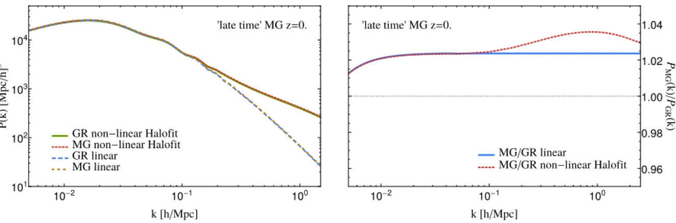
Boltzmann codes to estimate the non-linear contribution which corrects the linear power spectrum as a function of scale and time. We will use the Halofit fitting function as a way of approximating the non-linear power spectrum in our models even though it is really only valid for ΛCDM. In Fig.2, the left panel shows a comparison between the linear and non-linear power spectra calculated by MGCAMB in two different models, our fiducial late-time model (as from Table 1) and GR, both sharing the same ΛCDM parameters. At small length scales (large k), the non-linear deviation is clearly visible at scales k &0.3 h/Mpc and both MG and GR seem to overlap due to the logarithmic scale used. In the right panel, we can see the ratio between MG and GR for both linear and non-linear power spectra, using the same 5ΛCDMparameters{Ωm,Ωb, h, As, ns}. We can see clearly that MG in the non-linear regime, using the standard Halofit, shows a distinctive feature at scales in between 0.2 .k .2. This feature however, does not come from higher order perturbations induced by the modified Poisson equations (2,4), because Halofit, as explained above, is calibrated with simulations within theΛCDM model and does not contain any information from Modified Gravity. The feature seen here is caused by the different growth rate of perturbations in Modified Gravity, that yields then a different evolution of non-linear structures.
GR non-linear Halofit MG non-linear Halofit GR linear
MG linear
10-2 10-1 100
101 102 103 104
k@hMpcD
P
H
k
L@
Mpc
h
D
3
'late time' MG z=0.
MGGR linear
MGGR non-linear Halofit
10-2 10-1 100
0.96 0.98 1.00 1.02 1.04
k@hMpcD
P
MG
H
k
L
P
GR
H
k
L
'late time' MG z=0.
Figure 2. Left: matter power spectra computed with MGCAMB (linear) and MGCAMB+Halofit (non-linear), illustrating the impact of non-linearities at different scales. As an illustrative example, MG in this plot corresponds to the fiducial model in the late-time parametrization defined in Eq. (9). All curves are computed atz= 0. The green solid line is the GR fiducial in the non-linear case, the blue long-dashed line is also GR but in the linear case. The short-dashed red line is the MG fiducial in the non-linear case and the medium-dashed brown line the MG fiducial in the linear case. Right: in order to have a closer look at small scales, we plot here the ratio of the MG power spectrum to the GR power spectrum for the linear (blue solid) and non-linear (red short-dashed) cases separately. The blue solid line compared to the horizontal grey dashed line, shows the effect of Modified Gravity when taking only linear spectra into account. While the red dashed line, which represents the non-linear case, shows that the ratio to GR presents clearly a bump that peaks aroundk≈1.0h/Mpc, meaning that the power spectrum in MG differs at most 4% from the non-linear power spectrum in GR. We will see later that we are able to discriminate between these two models using future surveys, especially when non-linear scales (k&0.1h/Mpc) are included.
2. Prescription for mildly non-linear scales including screening
denoted asPnlHS
PnlHS(k, z) =
PHMG(k, z) +cnlSL2(k, z)PHGR(k, z) 1 +cnlS2L(k, z)
, (13)
with
S2L(k, z) = k3
2π2PLMG(k, z) s
. (14)
The weighting functionSLused in the interpolation quantifies the onset of non-linear clustering and it is constructed using the linear power spectrum in Modified Gravity (PLMG). The constantcnl and the constant exponentsare free parameters. In Figure3we show the ratioPnlHS/PHGR, which illustrates the relative difference between the non-linear HS prescription in MG and the Halofit non-linear power spectrum in GR, for different values ofcnl (left panel) and different values of s (right panel). The parametercnl controls at which scale there is a transition into a non-linear regime in which standard GR is valid (this can be the case when a screening mechanism is activated);scontrols the smoothness of the transition and is in principle a model and redshift dependent quantity. When cnl = 0 we recover the Modified Gravity power spectrum with HalofitPHMG; whencnl→ ∞we recover the non-linear power spectrum in GR calculated with HalofitPHGR. In [41,47, 48], thecnl ands constants were obtained fitting expression (13) to N-Body simulations or to a semi-analytic perturbative approach. In the case off(R), s= 1/3 seems to match very well the result from simulations up to a scale of k= 0.5h/Mpc [48]. A relatively good agreement up to such small scales is enough for our purposes. In the absence of N-Body simulations or semi-analytic methods available for the models investigated in this work, we will assume unity for both parameters, which is a natural choice, and we will test in Section VI Chow our results vary for different values of these parameters, namely cnl = {0.1,0.5,1,3} and s ={0,1/3,2/3, 1}. This will give a qualitative estimate of the impact of non-linearities on the determination of
cosmological parameters.
PHMG Hcnl=0L
cnl=0.5
cnl=1
cnl=10
cnl=1´108
10-2 10-1 100
0.96 0.98 1.00 1.02 1.04
k@hMpcD
PnlHS
H
k
L
PHGR
H
k
L
'late time' MG z=0.
s=1
PHMGHcnl=0L
s=0 s=0.33 s=0.66 s=1
10-2 10-1 100
0.96 0.98 1.00 1.02 1.04
k@hMpcD
PnlHS
H
k
L
PHGR
H
k
L
'late time' MG z=0.
cnl=1
Figure 3. The ratio of the Modified Gravity non-linear power spectrum using the HS prescription by [15] (PnlHS) with respect to the GR+Halofit fiducial non-linear power spectrumPHGR, for different values ofcnl(left panel) ands(right panel), illustrated in Eqns.(13, 14). The valuecnl = 0(green solid line) corresponds to MG+HalofitPHMG. All curves are calculated atz = 0.
Left: We show the ratio forcnl ={0.5,1.0,10,108}, plotted as short-dashed red, medium-dashed blue, short-dashed brown and medium-dashed purple lines respectively. Whencnl→ ∞, Eqn. (13) corresponds to the limit of PHGR and therefore the ratio is just 1. The effect of the HS prescription is to grasp some of the features of the non-linear power spectrum at mildly non-linear scales induced by Modified Gravity, taking into account that at very small scales, a screening mechanism might yield again just a purely GR non-linear power spectrum. The parametercnl interpolates between these two cases. Right: in this panel we show the effect of the parameter s, for s ={0,0.33,0.66,1} (short-dashed red, medium-dashed blue, short-dashed brown and long-dashed purple, respectively). Both parameters need to be fitted with simulations in order to yield a reliable match with the shape of the non-linear power spectrum in Modified Gravity, as it was done in [47] and references therein. The grey dashed line marks the constant value of 1.
IV. FISHER MATRIX FORECASTS
matrix formalism to two different probes, Galaxy Clustering (GC) and Weak Lensing (WL), which are the main cosmological probes for the future Euclid satellite [52]. The background and perturbations quantities we use in the following equations are computed with a version of MGCAMB[12,22] modified in order to account for the binning and the parameterizations described in SectionII.
A. Future large scale galaxy redshift surveys
In this work we choose to present results on some of the future galaxy redshift surveys, which are planned to be started and analyzed within the next decade. Our baseline survey will be the Euclid satellite [2, 53]. Euclid2 is a European Space Agency medium-class mission scheduled for launch in 2020. Its main goal is to explore the expansion history of the Universe and the evolution of large scale cosmic structures by measuring shapes and redshifts of galaxies, covering 15000deg2of the sky, up to redshifts of about
z∼2. It will be able to measure up to 100 million spectroscopic redshifts which can be used for Galaxy Clustering measurements and 2 billion photometric galaxy images, which can be used for Weak Lensing observations (for more details, see [2,53]). We will use in this work the Euclid Redbook specifications for Galaxy Clustering and Weak Lensing forecasts [53], some of which are listed in Tables2and 3and the rest can be found in the above cited references.
Another important future survey will be the Square Kilometer Array (SKA)3, which is planned to become the world’s largest radiotelescope. It will be built in two phases, phase 1 split into SUR in Australia and SKA1-MID in South Africa and SKA2 which will be at least 10 times as sensitive. The first stage is due to finish observations around the year 2023 and the second phase is scheduled for 2030 (for more details, see [54–57]). The first phase SKA1, will be able to measure in an area of 5000deg2of the sky and a redshift of up to
z∼0.8an estimated number of about 5×10⁶ galaxies; SKA2 is expected to cover a much larger fraction of the sky (∼30000deg2), will yield much deeper
redshifts (up toz ∼2.5) and is expected to detect about 109 galaxies with spectroscopic redshifts [55]. SKA1 and SKA2 will also be capable of performing radio Weak Lensing experiments, which are very promising, since they are expected to be less sensitive to systematic effects in the instruments, related to residual point spread function (PSF) anisotropies [58]. In this work we will use for our forecasts of SKA1 and SKA2, the specifications computed by [55] for GC and by [58] for WL. The numerical survey parameters are listed in Tables2 and3, while the galaxy biasb(z) and the number density of galaxiesn(z), can be found in the references mentioned above.
We will also forecast the results from DESI4, a stage IV, ground-based dark energy experiment, that will study large scale structure formation in the Universe through baryon acoustic oscillations (BAO) and redshift space distortions (RSD), using redshifts and positions from galaxies and quasars [59–61]. It is scheduled to start in 2018 and will cover an estimated area in the sky of about 14000deg2. It will measure spectroscopic redshifts for four different classes of objects, luminous red galaxies (LRGs) up to a redshift ofz = 1.0, bright [O II] emission line galaxies (ELGs) up to z= 1.7, quasars (QSOs) up to z∼3.5 and at low redshifts (z∼0.2) magnitude-limited bright galaxies (BLGs). In total, DESI will be able to measure more than 30 million spectroscopic redshifts. In this paper we will use for our forecasts only the specifications for the ELGs, as found in [59], since this observation provides the largest number density of galaxies in the redshift range of our interest. We cite the geometry and redshift binning specifications in Table2, while the galaxy number density and bias can be found in [59].
B. Galaxy Clustering
The distribution of galaxies in space is not perfectly uniform. Instead it follows, up to a bias, the underlying matter power spectrum so that the observed power spectrumPobs (the Fourier transform of the real-space two point correlation function of the galaxy number counts) is closely linked to the dark matter power spectrum P(k). The observed power spectrum however also contains additional effects like redshift-space distortions due to velocities and a suppression of power due to redshift-uncertainties. Here we follow [50], neglecting further relativistic and observational effects, and write the observed power spectrum as
Pobs(k, µ, z) =D 2
A,f(z)H(z) D2
A(z)Hf(z)
b2(z)(1 +βd(z)µ2)2e−k2µ2(σr2+σ
2
v)P(k, z) . (15)
Pobs(k, µ, z)is the observed power spectrum as a function of the redshiftz, the wavenumberkand ofµ≡cosα, where α is the angle between the line of sight and the 3D-wavevector~k. This observed power spectrum contains all the
cosmological information about the background and the matter perturbations as well as corrections due to redshift-space distortions, geometry and observational uncertainties. In the formula, the subscriptf denotes the fiducial value of each quantity, P(k, z) is the matter power spectrum, DA(z)is the angular diameter distance, H(z)the Hubble function andβd(z)is the redshift space distortion factor, which in linear theory is given by βd(z) =f(z)/b(z), with f(z)≡dlnG/dlnarepresenting the linear growth rate of matter perturbations andb(z)the galaxy bias as a function of redshift, which we assume to be local and scale-independent. The exponential factor represents the damping of the observed power spectrum, due to two different effects: σzan error induced by spectroscopic redshift measurement errors, which translates into an uncertainty in the position of galaxies at a scale of σr = σz/H(z)and σv which is the dispersion of pairwise peculiar velocities which are present at non-linear scales and also introduces a damping scale in the mapping between real and redshift space. We marginalize over this parameter, similarly to what [10] and others have done, and we take as fiducial value σv = 300km/s, compatible with the estimates by [62]. We also include the Alcock-Paczynski effect [63], by which the kmodes and the angle cosineµperpendicular and parallel to the line-of-sight get distorted by geometrical factors related to the Hubble function and the angular diameter distance [64,65].
We can then write the Fisher matrix for the galaxy power spectrum in the following form [50,66]:
Fij= Vsurvey
8π2 ˆ +1
−1 dµ
ˆ kmax
kmin
dk k2∂lnPobs(k, µ, z) ∂θi
∂lnPobs(k, µ, z) ∂θj
n(z)P
obs(k, µ, z) n(z)Pobs(k, µ, z) + 1
2
. (16)
HereVsurvey is the volume covered by the survey and contained in a redshift slice∆zandn(z)is the galaxy number density as a function of redshift. We will consider the smallest wavenumberkmin to bekmin= 0.0079h/Mpc , while the maximum wavenumber will bekmax= 0.15h/Mpc for the linear forecasts andkmax= 0.5h/Mpc for the non-linear forecasts. In the above formulation of the Galaxy Clustering Fisher matrix, we neglect the correlation among different redshift bins and possible redshift bin uncertainties as was explored recently in [67], we will use for our forecasts the more standard recipe specified in the Euclid Redbook [53].
Parameter Euclid DESI-ELG SKA1-SUR SKA2 Description
Asurvey 15000 deg2 14000 deg2 5000 deg2 30000 deg2 Survey area in the sky σz 0.001 0.001 0.0001 0.0001 Spectroscopic redshift error {zmin, zmax} {0.65, 2.05} {0.65, 1.65} {0.05, 0.85} {0.15, 2.05} Min. and max. limits for redshift bins
∆z 0.1 0.1 0.1 0.1 Redshift bin width
Table 2. Specifications for the spectroscopic galaxy redshift surveys used in this work. The number density of tracersn(z)
and the galaxy biasb(z), can be found for SKA in [55] and for DESI in reference [59].
C. Weak Lensing
Light propagating through the universe is deflected by variations in the Weyl potentialΦ + Ψ, leading to distortions in the images of galaxies. In the regime of small deflections (Weak Lensing) we can write the power spectrum of the shear field as
Cij(`) = 9 4
ˆ ∞
0
dz Wi(z)Wj(z)H 3(z)Ω2
m(z)
(1 +z)4 [Σ(`/r(z), z)]Pm(`/r(z)). (17) In this expression we used Eqn. (4) to relate the Weyl potential toΣand to the matter power spectrumPm and we use the Limber approximation to write down the conversionk=`/r(z), wherer(z)is the comoving distance given by
r(z) =c ˆ z
0 dz˜
H(˜z). (18)
The indices i, j stand for each of the Nbin redshift bins, such that Cij is a matrix of dimensionsNbin× Nbin. The window functionsWi are given by
W(z) =
ˆ ∞
z dz˜
1−r(z)
r(˜z)
n(˜z) (19)
n(z)∝z2exp−(z/z0)3/2
. (20)
Here the median redshiftzmed andz0 are related byzmed=
√
2z0. The Weak Lensing Fisher matrix is then given by a sum over all possible correlations at different redshift bins [49],
Fαβ=fsky `max
X
` X
i,j,k,l
(2`+ 1)∆` 2
∂Cij(`) ∂θα
Cov−1 jk
∂Ckl(`) ∂θβ
Cov−1
li . (21)
The prefactor fsky is the fraction of the sky covered by the survey. The upper limit of the sum, `max, is a high-multipole cutoff due to our ignorance of clustering and baryon physics on small scales, similar to the role ofkmax in Galaxy Clustering. In this work we choose`max = 1000for the linear forecasts and `max = 5000 for the non-linear forecasts (this cutoff is not necessarily reached at all multipoles`, as what matters is the minimum scale between`max andkmax, as we discuss below; see also [3]). In Eqn. (21), Covij is the corresponding covariance matrix of the shear power spectrum and it has the following form:
Covij(`) =Cij(`) +δijγint2 n −1
i +Kij(`) (22)
whereγint is the intrinsic galaxy ellipticity, whose value can be seen in Table3 for each survey. The shot noise term n−i1 is expressed as
ni= 3600
180 π
2
nθ/Nbin (23)
with nθ the total number of galaxies per arcmin2 and the index istanding for each redshift bin. Since the redshift bins have been chosen such that each of them contains the same amount of galaxies (equi-populated redshift bins), the shot noise term is equal for each bin. The matrixKij(`)is a diagonal “cutoff” matrix, discussed for the first time in [3] whose entries increase to very high values at the scale where the power spectrum P(k)has to be cut to avoid the inclusion of uncertain or unresolved non-linear scales. We choose to add this matrix to have further control on the inclusion of non-linearities. Without this matrix, due to the redshift-dependent relation betweenkand`, a very high `max would correspond at low redshifts, to a very highkmax where we do not longer trust the accuracy of the non-linear power spectrum. Therefore, the sum in Eqn. (21) is limited by the minimum scale imposed either by`max or by kmax, which is the maximum wavenumber considered in the matter power spectrum P(k, z). As we did for Galaxy Clustering, we use for linear forecastskmax= 0.15and for non-linear forecastskmax= 0.5.
Parameter Euclid SKA1 SKA2 Description
fsky 0.364 0.121 0.75 Fraction of the sky covered σz 0.05 0.05 0.05 Photometric redshift error
nθ 30 10 2.7 Number of galaxies per arcmin
γint 0.22 0.3 0.3 Intrinsic galaxy ellipticity z0 0.9 1.0 1.6 Median redshift over
√
2
Nbin 12 12 12 Total number of tomographic redshift bins
Table 3. Specifications for the Weak Lensing surveys Euclid, SKA1 and SKA2 used in this work. Other needed quantities can be found in the references cited in sectionIV A. For all WL surveys we use a redshift range betweenz= 0.5andz= 3.0, using 6 equi-populated redshift bins.
D. Covariance and correlation matrix and the Figure of Merit
The covariance matrix is defined for ad-dimensional vectorpof random variables as
C=h∆p∆pTi (24)
with ∆p = p− hpi and the angular brackets h i representing an expectation value. The matrix C, with all its off-diagonal elements set to zero, is called the variance matrix V and contains the square of the errorsσi for each parameterpi
The Fisher matrixFis the inverse of the covariance matrix
F=C−1 . (26)
The correlation matrixPis obtained from the covariance matrixC, in the following way
Pij = Cij p
CiiCjj
. (27)
If the covariance matrix is non-diagonal, then there are correlations among some elements ofp. We can observe this also by plotting the marginalized error ellipsoidal contours. The orientation of the ellipses can tell us if two variables piandpj are correlated (Pij>0), corresponding to ellipses with 45 degree orientation to the right of the vertical line or if they are anti-correlated (Pij <0), corresponding to ellipses oriented 45 degrees to the left of the vertical line.
To summarize the information contained in the Fisher/covariance matrices we can define a Figure of Merit (FoM). Here we choose the logarithm of the determinant, while another possibility would be the Kullback-Leibler divergence, which is a measure of the information entropy gain, see AppendixE.
The square-root p
det(C) of the determinant of the covariance matrix is proportional to the volume of the error ellipsoid. We can see this if we rotate our coordinate system so that the covariance matrix is diagonal, C = diag(σ21, σ22, . . . σ2d), then det(C) =
Q iσ
2
i and (1/2) ln(det(C)) = ln Q
iσi would indeed represent the loga-rithm of an error volume. Thus, the smaller the determinant (and therefore alsoln(det(C))), the smaller is the ellipse and the stronger are the constraints on the parameters. We define
FoM =−1
2ln(det(C)), (28)
with a negative sign in front such that stronger constraints lead to a higher Figure of Merit. In the following, the value of the FoM reported in all tables will be obtained including only the dark energy parameters (i.e. the (µi, ηi) sub-block for the binned case and the (µ, η) sub-block in the smooth functions case), after marginalizing over all other parameters. The FoM allows us to compare not only the constraining power of different probes but also of the different experiments. As the absolute value depends on the details of the setup, we define the relative figure of merit between probe a and probeb: FoMa,b =−1/2 ln(det(Ca)/det(Cb)) = FoMa−FoMb and we fix our reference case (probeb), for each parametrization, to the Galaxy Clustering observation using linear power spectra with the Euclid survey (labeled as ‘Euclid Redbook GC-lin’ in all figures and tables). The FoM has units of ‘nits’, since we are using the natural logarithm. These are similar to ‘bits’, but ‘nits’ are counted in baseeinstead of base 2.
An analogous construction allows us to study quantitatively the strength of the correlations encoded by the corre-lation matrixP. We define the ‘Figure of Correlation’ (FoC) as:
FoC =−1
2ln(det(P)). (29)
If the parameters are independent, i.e. fully decorrelated, then Pis just the unit matrix and ln(det(P)) = 0. Off-diagonal correlations will decrease the logarithm of the determinant, therefore making the FoC larger. From a geometrical point of view, the determinant expresses a volume spanned by the vector of (normalized) variables. If these variables are independent, the volume would be maximal and equal to one, while if they are strongly linearly dependent, the volume would be squeezed and in the limit where all variables are effectively the same, the volume would be reduced to zero. Hence, a more positive FoC indicates a stronger correlation of the parameters.
E. CMBPlanck priors
θis usually the ratio of sound horizon to the angular diameter distance at the time of decoupling. Since calculating the decoupling timezCMBis relatively time consuming, as it involves the minimization of the optical transfer function, COSMOMCuses instead an approximate quantityθMC based on the following fitting formula from [70]
zCMB= 1048×(1 + 0.00124ωb−0.738)
× 1 + 0.0783ωb−0.238/(1 + 39.5ω0.763b )
×(ωd+ωb)0.560/(1+21.1ω 1.81
b )
(30)
whereωd≡(Ωc+ Ων)h2. The sound horizon is defined as
rs(zCMB) =cH0−1
ˆ ∞
zCMB dz cs
E(z) (31)
where the sound speed is cs = 1/ q
3(1 +Rba)with the baryon-radiation ratio being Rba = 3ρb/4ργ. Rb = 31500Ωbh2(TCMB/2.7K)−4. However, CAMB approximates it asRba= 30000aΩbh2.
Therefore we first marginalize the covariance matrix over the nuisance parameters and the parameter τ, which cannot be constrained by LSS observations. Then, we invert the resulting matrix, to obtain a Planck prior Fisher matrix and then use a Jacobian to convert between the MCMC parameter basisΘiand the GC-WL parameter basisθi. We use the formulas above for the sound horizonrsand the angular diameter distancedAto calculate the derivatives ofθMC with respect to the parameters of interest. Our Jacobian is then simply (see AppendixAfor details)
Jij = ∂Θi
∂θj
. (32)
V. RESULTS: EUCLID FORECASTS FOR REDSHIFT BINNED PARAMETERS
In this section we analyze the Modified Gravity functions µ(a) and η(a), described in Section II, when they are allowed to vary freely in five redshift bins.
For this purpose, we calculate a Fisher matrix of fifteen parameters: five for the standard ΛCDM parameters
{Ωm,Ωb, h,ln 1010As, ns}, five forµ (one for each bin amplitudeµi) and five for η (one for each bin amplitude ηi), corresponding to the 5 redshift bins z={0-0.5, 0.5-1.0, 1.0-1.5, 1.5-2.0, 2.0-2.5}. The fiducial values for all fifteen parameters were calculated running a Markov-Chain-Monte-Carlo with Planck likelihood data and can be found in Table1.
We first show the constraints on our 15 parameters for Galaxy Clustering (GC) forecasts in subsectionV A, while in subsection V B we report results for Weak Lensing (WL). In subsection V C, we comment on the combination of forecasts for GC+WL together with Planckdata. All forecasts are performed using Euclid Redbook specifications. Other surveys will be considered for the other two time parameterizations in sectionVI A 4andVI B 2. For each case, we show the correlation matrix obtained from the covariance matrix and argue that the redshift-binned parameters show a strong correlation, therefore we illustrate the decorrelation procedure for the covariance matrix in subsection V Dwhere we also include combined GC+WL and GC+WL+Planckcases.
A. Euclid Galaxy Clustering Survey
ΩcΩbnsAs h μ1μ2μ3μ4μ5η1η2 η3η4η5 Ωc
Ωb
ns
As
h
μ1 μ2 μ3 μ4 μ5 η1 η2 η3 η4 η5
-1.0
-0.5 0 0.5 1.0
(linear)GC: Correlation Matrix
ΩcΩbnsAs h μ1μ2 μ3μ4μ5 η1η2η3 η4η5 Ωc
Ωb
ns
As
h μ1 μ2 μ3 μ4 μ5 η1 η2 η3 η4 η5
-1.0 -0.5 0 0.5 1.0 (non-linear)GC: Correlation Matrix
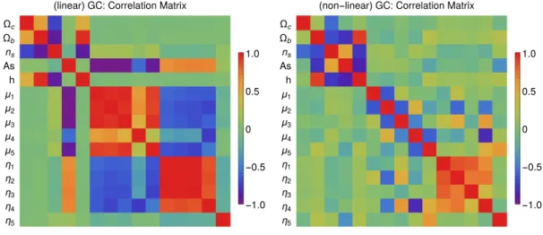
Figure 4. Correlation matrixPdefined in (27) obtained from the covariance matrix in the MG-binning case, for a Galaxy Clustering Fisher forecast using Euclid Redbook specifications. Left panel: Linear forecasts. Here there are strong positive correlations among theµiandηiparameters and anti-correlations betweenln 1010Asand theµiparameters, as well as between
µi andηi. The FoC in this case is≈65. (see Eqn. (29) for its definition). Right panel: Non-linear forecasts using the HS prescription. Interestingly, the anti-correlations betweenln 1010As andµihave disappeared, as well as the correlations among theµi parameters. The FoC is in this case≈32, meaning that the variables are much less correlated than in the linear case. This is due to the fact that taking into account non-linear structure formation breaks degeneracies between the primordial amplitude parameter and the modifications to the Poisson equation.
We calculate the Fisher matrix for the 15 parametersθ={Ωm,Ωb, h,ln 1010As, ns, µi, ηi}whereηiandµi represent ten independent parameters, one for each function at each of the 5 redshift bins corresponding to the redshifts z={0-0.5, 0.5-1.0, 1.0-1.5, 1.5-2.0, 2.0-2.5}. As a standard procedure, we marginalize over the unknown bias parameters. From the covariance matrix, defined previously in Eqn. (24), we obtain the correlation matrixPijdefined in Eqn. (27) for the set of parametersθi. In Figure 4 we show the matrixPij in the linear (left panel) and non-linear-HS (right panel) cases. Redder (bluer) colors signal stronger correlations (anti-correlations).
A covariance matrix that contains strong correlations among parameter A and B, means that the experimental or observational setting has difficulties distinguishing between A and B for the assumed theoretical model, i.e. this represents a parameter degeneracy. Therefore if for example parameter A is poorly constrained, then parameter B will be badly constrained as well. The appearance of correlations among parameters is linked to the non-diagonal elements of the covariance matrix. Subsequently, this means that the fully marginalized errors on a single parameter, will be larger if there are strong correlations and will be smaller (closer to the value of the fully maximized errors) if the correlations are negligible.
In the linear case, µi and ηi parameters show correlations among each other, while the primordial amplitude parameterln 1010A
sexhibits a strong anti-correlation with all theµi. This can be explained considering that a larger growth of structures in linear theory can also be mimicked with a larger initial amplitude of density fluctuations.
Interestingly, including non-linear scales in the analysis (right panel of Fig. 4) leads to a strong suppression of the correlations among the µi. Also the correlation between these andln 1010As is suppressed as a change in the initial amplitude of the power spectrum is not able to compensate for a modified Poisson equation when non-linear evolution is considered.
As discussed in SectionIV D, we can also express the difference between the correlation matrix of the linear forecast and the non-linear forecast in a more quantitative way, by computing the determinant of the correlation matrix, or equivalently the FoC (29). If the correlations were negligible, this determinant would be equal to one (and therefore its FoC would be 0), while if the correlations were strong, the determinant would be closer to zero with a corresponding large positive value of the FoC. For the linear forecast, the FoC is about62, while for the non-linear forecast, it is much smaller at approximately35. In Table4 we show the 1σconstraints obtained onln (1010As)and on theµ
i and ηi parameters, both in the linear and non-linear cases for a Euclid Redbook GC survey (top rows). While linear GC alone (kmax= 0.15 h/Mpc) is not very constraining in any bin, the inclusion of non-linear scales (kmax= 0.5 h/Mpc) drastically reduces errors on theµi parameters: the first three bins in µi (0. < z < 1.5 ) are the best constrained, to less than 10%, with the corresponding ηi constrained at 20% by non-linear GC alone. This is also visible in the FoM which increases by 19 nits (‘natural units’, similar to bits but using basee instead of base 2), nearly 4 nits per redshift bin on average, when including the non-linear scales. The fact that the error on ln 1010A
90% to 0.68% shows that the decorrelation induced by the non-linearities breaks the degeneracy with the amplitude and therefore improves considerably the determination of cosmological parameters. This shows that it is important to include non-linear scales in GC surveys (and not only in Weak Lensing ones, which is usually more expected and will be shown in the next subsection).
Euclid(Redbook) `As µ1 µ2 µ3 µ4 µ5 η1 η2 η3 η4 η5 MG FoM
Fiducial 3.057 1.108 1.027 0.973 0.952 0.962 1.135 1.160 1.219 1.226 1.164 relative
GC (lin) 160% 119% 159% 183% 450% 1470% 509% 570% 586% 728% 3390% 0
GC (nl-HS) 0.8% 7.0% 6.7% 10.9% 27.4% 41.1% 20% 24.3% 19.9% 38.2% 930% 19
WL (lin) 640% 165% 2210% 4150% 13100% 22500% 2840% 3140% 8020% 29300% 39000% -27
WL (nl-HS) 7.3% 188% 255% 419% 222% 206% 330% 488% 775% 8300% 9380% -10
GC+WL (lin) 11.3% 5.8% 10% 19.2% 282% 469% 7.9% 9.6% 16.1% 276% 2520% 12
GC+WL+Planck (lin) 1.1% 3.4% 4.8% 7.8% 9.3% 13.1% 6.2% 7.7% 9.1% 12.7% 23.6% 27
GC+WL (nl-HS) 0.8% 2.2% 3.3% 8.2% 24.8% 34.1% 3.6% 5.1% 8.1% 25.4% 812% 24
GC+WL+Planck
(nl-HS) 0.3% 1.8% 2.5% 5.8% 7.8% 10.3% 3.2% 4.1% 5.9% 9.6% 19.5% 33
GC+WL+Planck
(nl-Halofit) 0.4% 2.0% 2.4% 5.1% 7.4% 10.2% 3.5% 4.1% 5.8% 9.2% 18.9% 33
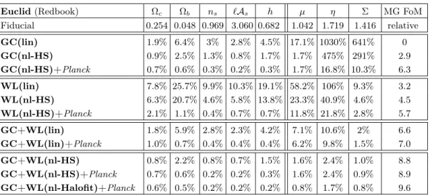
Table 4. 1σ fully marginalized errors (as a percentage of the corresponding fiducial) on cosmological parameters for Euclid (Redbook) Galaxy Clustering and Weak Lensing surveys, alone and combining the two probes. We compare forecasts using linear spectra (lin) and forecasts using the nonlinear HS prescription (nl-HS). In Galaxy Clustering, the cutoff is set tokmax = 0.15 h/Mpc in the linear case andkmax= 0.5h/Mpc in the non-linear case. For WL, the maximum cutoff in the linear case is at `max= 1000, while in the nl-HS case it is`max= 5000. At the bottom, we add on top aPlanck prior (see sectionIV E). For comparison, we also show in the last row the combined GC+WL+Planck, using just Halofit power spectra. The last column indicates the relative Figure of Merit (FoMa,b) of the MG parameters in nits (‘natural units’, i.e. using the natural logarithm),
with respect to our reference GC linear case, see (28) and surrounding text. A larger FoM indicates a more constraining probe. We notice a considerable improvement, in both GC and WL, when non-linearities are included. The combination GC+WL in the linear case constrains the MG parameters in the first two bins (z < 1.0 ) to less than 10%and includingPlanckpriors allows to access higher redshifts with the same accuracy. A significant improvement in the constraints is obtained when adding the non-linear regime, in agreement with the observed reduction in correlation seen in Figs. 4and 5. This is especially well exemplified by the error on`As≡ln(1010As), which reduces from 160% to 0.82%, from the linear to the non-linear forecast in
the GC case and from 640% to 7.3% in the WL case. Finally, we note that since we are showing errors onµandη, WL seems to be unfairly poor at constraining parameters. However, when converting this errors into errors onΣ, which is directly measured by WL, the constrains onΣ1,2,3 are slightly better, of the order of 40% for WL(nl-HS) as can be guess from the degeneracy directions shown in Fig.14. The FoM itself is nearly unaffected by the choice of{µ, η}vs{µ,Σ}as it is rotationally invariant.
B. Euclid Weak Lensing Survey
ΩcΩbnsAs h μ1μ2μ3μ4μ5η1η2 η3η4η5 Ωc
Ωb
ns
As
h μ1 μ2 μ3 μ4 μ5 η1 η2 η3 η4 η5
-1.0 -0.5 0 0.5 1.0 (linear)WL: Correlation Matrix
ΩcΩbnsAs h μ1μ2 μ3μ4μ5 η1η2η3 η4η5 Ωc
Ωb
ns
As h μ1 μ2 μ3 μ4 μ5 η1 η2 η3 η4 η5
-1.0 -0.5 0 0.5 1.0 (non-linear)WL: Correlation Matrix
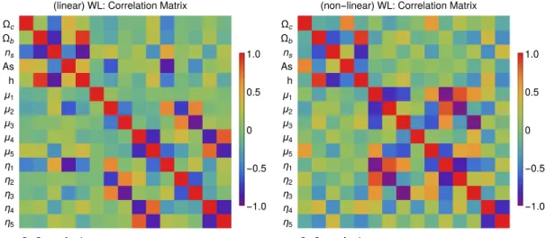
Figure 5. Correlation matrix obtained from the covariance matrix in the MG-binning case, for a Weak Lensing Fisher Matrix forecast using Euclid Redbook specifications. Left panel: linear forecasts. Strong anti-correlations are present between the
µiand theηiparameters for the same value of i in 2,3,4,5. The amplitudeln(1010As)parameter is mostly uncorrelated except withη1. The FoC (29) in this case is approximately69. Right panel: non-linear forecasts using the HS prescription. Here the same trend as in the linear case is present, with just subtle changes. The FoC in this case is about32, meaning that the variables are indeed less correlated than in the linear case. The parameterln(1010As) is effectively not correlated to other parameters, and the anti-correlation ofµi and theηifor the same value of the index i is present in the first three bins. The anti-correlation between these two sets of parameters is expected, since WL is sensitive to the Weyl potential Σ, which is a product ofµandη.
Table4shows the corresponding 1σmarginalized errors onln (1010As)and on theµ
iandηi, both in the linear and non-linear cases for a Euclid Redbook WL survey. As in the case of GC, linear WL cannot constrain alone any of the amplitudes of the Modified Gravity parametersµi andηi for any redshift bin. Being able to include non-linear scales improves constraints on the amplitudeln(1010A
s) by a factor 100. The 1σerrors onµi and ηi improve up to one order of magnitude, with the FoM increasing by 17 nits, although remaining quite unconstraining for Modified Gravity parameters in all redshift bins. Notice, however, that the 1σerror onµ1from WL in the linear case is slightly smaller than in the non-linear case. This can be attributed to the fact that in the linear case, µ1 is uncorrelated to any other parameter, as shown in Figure5and on that specific bin (0 < z < 0.5) non-linearities don’t seem to improve the constraints on this parameter.
C. Combining Euclid Galaxy Clustering and Weak Lensing, withPlanck data
The combination of Galaxy Clustering and Weak Lensing is expected to be very powerful for Modified Gravity parameters as they measure two different combinations of µand η, thus breaking their degeneracy as illustrated in Fig. 14. This is shown in Table4, where the sensitivity drastically increases with respect to the two separate probes, especially in the low redshifts bins(0. < z <1.5), where the lensing signal is dominant. Adding non-linearities further doubles the FoM. ThePlanckdata constrains mostly the standardΛCDMparameters and has only a limited ability to constrain the MG sector. However, the additional information breaks parameter degeneracies and in this way significantly decreases the uncertainties on all parameters, so that the linear GC+WL+Planckis comparable to the non-linear GC+WL. Also, quantitatively, the correlation among parameters is reduced by combining GC+WL with Planck data. The FoC in this case is of ≈ 22. We also see in Table4 that the differences between the non-linear prescription adopted here (nl-HS) and a straightforward application of Halofit to the MG case (nl-Halofit) is not very large. We will investigate further the impact of the parameters used in the non-linear prescription in sectionVI C.
D. Decorrelation of covariance matrices and the Zero-phase Component Analysis
without including non-linearities, however, it is interesting to investigate how we can completely decorrelate the parameters, identifying in this way those parameter combinations which are best constrained by data.
Given again ad-dimensional vectorpof random variables (our originally correlated parameters), we can calculate its covariance matrixC defined in Eqn. (24). The process of decorrelation is the process of making the matrix C a diagonal matrix.
Let us define some important identities. The covariance matrix can be decomposed in its eigenvalues (the elements of a diagonal matrixΛ) and eigenvectors (the rows of an orthogonal matrixU).
C=UΛUT ⇔ F=UΛ−1UT , (33)
whereFis the Fisher Matrix.
It is possible to show that applying a transformation matrixW to the pparameter vector, thus obtaining a new vector of variables q = W p, the covariance matrix of the transformed vector q is whitened (i.e. it is the identity matrix, and whitening is defined as the process of converting the covariance matrix into an identity matrix)
˜
C=Wh∆ˆp∆ˆpTiWT =h∆ˆq∆ˆqTi (34)
=1 .
This means that the transformedqparameters are decorrelated, since their correlation matrix is diagonal. The choice ofW is not unique as several possibilities exist; we focus on a particular choice in the rest of the paper referred to as Zero-phase Component Analysis (ZCA, first introduced by [73] in the context of image processing), but we show two other possible choices and their effect on the analysis in AppendixC.
Zero-phase Component Analysis (sometimes also called Mahalanobis transformation [74]) is a specific choice of decorrelation method that minimizes the squared norm of the difference between theqi and the pi vector k~p−~qk, under the constraint that the vector~qshould be uncorrelated [74]. In this way the uncorrelated variablesqwill be as close as possible to the original variablespin a least squares sense. This is achieved by using theW matrix:
W ≡F1/2 . (35)
Then in this case, the covariance matrix is whitened, by following Eqn. (34):
˜
C=F1/2F−1F1/2=1 . (36)
In our case, since we do not want to whiten, but just decorrelate the covariance matrix, we renormalize theW matrix by multiplying with a diagonal matrixNjj ≡Pj(W
−2
ij ), such that the sum of the square of the elements on each row of the new weighting matrix W˜ ≡N W, is equal to unity; therefore the final transformed covariance is still diagonal but is not the identity matrix:
˜
C= ˜W CW˜ =N21 (37)
and at the same time we ensure that the vector of new variables qi will have the same norm as the old vector of variablespi.
1. ZCA for Galaxy Clustering
From Fig.4we can see that the correlations are present in sub-blocks, one for the standardΛCDMparameters and another one for the Modified Gravity parameters. The exception lies in the linear case where`As≡ ln (1010As)is strongly anti-correlated with all the µi and positively correlated with the ηi. To use a more objective criterion, we choose the10×10block of MG parameters µi and ηi with parameter indices 6 to 15, and only add to this block a ΛCDMparameter with indexaif the following condition is satisfied:
i=15 X
i=6
(Pai)2≥1
with the amplitude), but for consistency we will use the same vector of 11 parameters pi = {`As, µi, ηi} for our decorrelation procedure. Therefore we will also have 11 transformed uncorrelated qi parameters, function of the originalpiparameters, in all the cases presented below.
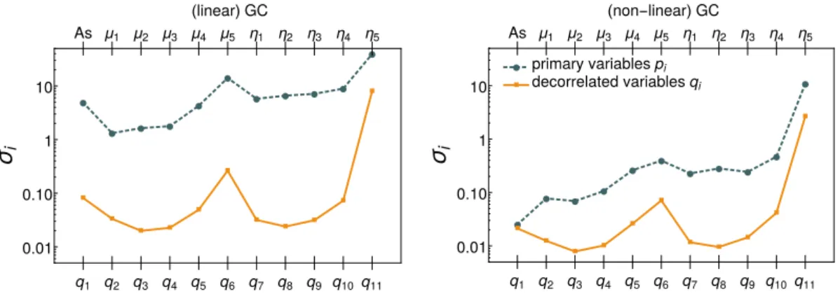
Figure 6 shows the coefficients that relate the qi parameters to the originalpi ones, in the linear (left panel) and the non-linear (right panel) cases, also shown explicitly in Tables 11 and12 of Appendix D. We plot in Figure 7 a comparison between the 1σ errors on the primary parameters pi (represented by circles connected with dark green dashed lines) and the decorrelated parametersqi (represented by squares connected with orange solid lines). In the linear case (left panel), we can see that the errors on the qi parameters are 2 orders of magnitude better than the errors on thepi parameters. In the non-linear case (right panel) the improvement is of at most 1 order of magnitude and that for a completely decorrelated parameter like `As, the error on its corresponding qi is exactly the same. This shows that a decorrelation procedure is still worth to do, even when including the non-linear regime, even if the degeneracy with the amplitude is already completely broken thanks to the non-linear prescription. The fact that the curve of 1σ errors for the qi follows the same pattern as the curve for the pi errors, is due to the fact that we have used a ZCA decomposition (see SectionV D) and therefore the qi are as similar as possible to thepi.
As μ1 μ2 μ3 μ4 μ5 η1 η2 η3 η4 η5
q1
q2
q3
q4
q5
q6
q7
q8
q9
q10
q11
0 0.2 0.4 0.6 0.8 1.0 (linear)GC: Weight matrix
As μ1 μ2 μ3 μ4 μ5 η1 η2 η3 η4 η5
q1
q2
q3
q4
q5
q6
q7
q8
q9
q10
q11
0 0.2 0.4 0.6 0.8 1.0
(non-linear)GC: Weight matrix
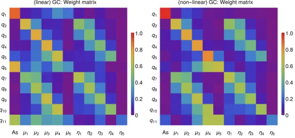
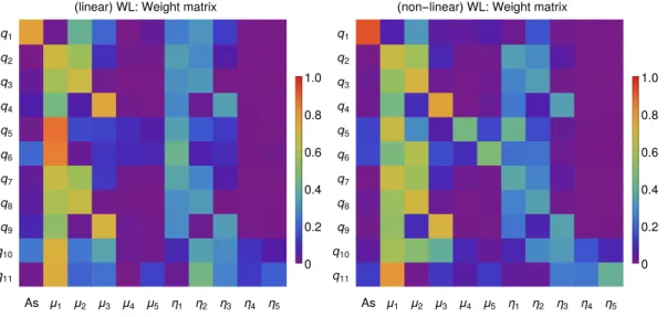
Figure 6. Entries of the matrixW that relates theqiparameters to the originalpiones, after applying the ZCA decorrelation of the covariance matrix in the linear and non-linear GC cases. This matrix shows for each new variable qi on the vertical axis, the coefficients of the linear combination of parametersµi, ηi andAs that give rise to that variableqi. The red (blue) colors, indicate a large (small) contribution of the respective variable on the horizontal axis. Left panel: linear forecast for Euclid Redbook specifications. Right panel: non-linear forecast for Euclid Redbook specifications, using the HS prescription. In both cases one can observe that mostqi parameters have only small or negligible contributions fromµ5 andη5, which are found to be the less constrained bins.
We are interested in finding the best combination of primary parameters pi giving rise to the best constrained uncorrelated parametersqi. In order to find the errors on the parametersqi, we need to look at the diagonal of the decorrelated covariance matrix C˜ expressed in Eqn. (37) and identify the qi parameters with the smallest relative errors (σqi/qi): we find than in the linear GC case, the best constrained combinations of primary parameters (ordered
from most to least constrained) are given approximately by:
q1= +0.9`As+ 0.32µ4
q3= +0.75µ2−0.29η1+ 0.50η2
q4=−0.25µ2+ 0.74µ3−0.32η2+ 0.49η3 q2= +0.70µ1−0.30µ2+ 0.52η1−0.36η2 .
(38)
●
● ● ●
● ●
● ● ● ●
●
■
■
■ ■
■ ■
■ ■ ■
■ ■
q1 q2 q3 q4 q5 q6 q7 q8 q9 q10 q11
0.01 0.10 1 10
As μ1 μ2 μ3 μ4 μ5 η1 η2 η3 η4 η5
σ
i(linear)GC
●
● ● ●
● ● ● ● ●
● ●
■ ■
■ ■
■ ■
■ ■ ■
■ ■
● primary variablespi
■ decorrelated variablesqi
q1 q2 q3 q4 q5 q6 q7 q8 q9 q10q11
0.01 0.10 1 10
As μ1 μ2 μ3 μ4 μ5 η1 η2 η3 η4 η5
σ
i(non-linear)GC
Figure 7. Results for a Euclid Redbook GC survey, with redshift-binned parameters, before and after applying the ZCA decorrelation. Each panel shows the 1σfully marginalized errors on the primary parameterspi(green dashed lines), and the 1σ
errors on the decorrelated parametersqi(orange solid lines). Left: linear forecasts, performed using linear power spectra up to a maximum wavenumberkmax= 0.15h/Mpc. Right: non-linear forecasts using non-linear spectra with the HS prescription up to a maximum wavenumberkmax= 0.5h/Mpc. In the linear case, the errors on the decorrelatedqiparameters are about 2 orders of magnitude smaller than for the primary parameters, while in the non-linear HS case, the improvement in the errors is of one order of magnitude. This means that applying a decorrelation procedure is worth even when non-linearities are considered. In both cases for GC, the least constrained parameters areµ5 andη5, corresponding to2.0< z <2.5.
q1 q3 q4 q2
As μ1 μ2 μ3 μ4 μ5 η1 η2 η3 η4 η5
-1.0
-0.5 0.0 0.5 1.0
coefficients
of
qi
(linear)GC: best constrained modes
q1 q4 q3 q2
As μ1 μ2 μ3 μ4 μ5 η1 η2 η3 η4 η5
-1.0
-0.5 0.0 0.5 1.0
coefficients
of
qi
(non-linear)GC: best constrained modes
Figure 8. Best constrained modes for a Euclid Redbook GC survey, with µ and η binned in redshift, after transforming into uncorrelated q parameters via ZCA. Each of the four best constrained parameters qi, shown in the panels, is a linear combination of the primary parameterspi. Theqi in the legends are ordered from left to right, from the best constrained to the least constrained.
non-linear case, are:
q1= +0.99`As
q4=−0.28µ2+ 0.76µ3−0.33η2+ 0.47η3 q3= +0.73µ2−0.32η1+ 0.49η2
q2= +0.68µ1−0.35µ2+ 0.52η1−0.37η2 .
(39)
2. ZCA for Weak Lensing
We apply the same decorrelation procedure to the WL case, obtaining theqvectors shown in the weight matrix of Figure9 again reported explicitly in Tables13and14in AppendixD.
As μ1 μ2 μ3 μ4 μ5 η1 η2 η3 η4 η5
q1
q2
q3
q4
q5
q6
q7
q8
q9
q10
q11
0 0.2 0.4 0.6 0.8 1.0
(linear)WL: Weight matrix
As μ1 μ2 μ3 μ4 μ5 η1 η2 η3 η4 η5
q1
q2
q3
q4
q5
q6
q7
q8
q9
q10
q11
0 0.2 0.4 0.6 0.8 1.0
(non-linear)WL: Weight matrix
Figure 9. Entries of the matrixW that relates theqiparameters to the originalpiones, after applying the ZCA decorrelation of the covariance matrix in the linear and non-linear WL cases. This matrix shows for each new variableqion the vertical axis, the coefficients of the linear combination of parametersµi,ηiandAsthat give rise to that variableqi. The red (blue) colors, indicate a large (small) contribution of the respective variable on the horizontal axis. Left panel: linear forecast for Weak Lensing Euclid Redbook specifications. Right panel: non-linear forecast for Weak Lensing Euclid Redbook specifications, using the HS prescription. As for GC, mostqiparameters have only small or negligible contributions fromµ5 andη5, which are found to be the less constrained bins.
In Figure10we show the comparison between the errors on the primary parameterspi and the de-correlated ones qi. As for the GC case, the errors in the linear case improve by 2 orders of magnitude after applying the decorrelation procedure (left panel). In the non-linear case (right panel) the improvement is smaller, but still worth to do, especially to constrainq2, q3, q7, q8.
●
●
● ●
● ●
● ●
●
● ●
■
■ ■ ■
■ ■
■ ■ ■
■ ■
q1 q2 q3 q4 q5 q6 q7 q8 q9 q10q11
0.01 0.10 1 10 100 1000
As μ1 μ2 μ3 μ4 μ5 η1 η2 η3 η4 η5
σ
i(linear)WL
●
● ●
●
● ●
● ●
●
● ●
■
■ ■ ■
■ ■
■ ■
■ ■
■ ● primary variablespi
■ decorrelated variablesqi
q1 q2 q3 q4 q5 q6 q7 q8 q9 q10q11 0.01
0.10 1 10 100 1000
As μ1 μ2 μ3 μ4 μ5 η1 η2 η3 η4 η5
σ
i(non-linear)WL
Figure 10. Results for a Euclid Redbook WL survey, with redshift-binned parameters, before and after applying the ZCA decorrelation. Each panel shows the 1σfully marginalized errors on the primary parameterspi (green dashed lines), and the 1σerrors on the decorrelated parameters qi (orange solid lines). Left: Linear forecasts, performed with an`max = 1000and linear matter power spectra. Right: Non-linear forecasts using the non-linear spectra with the HS prescription, up to an
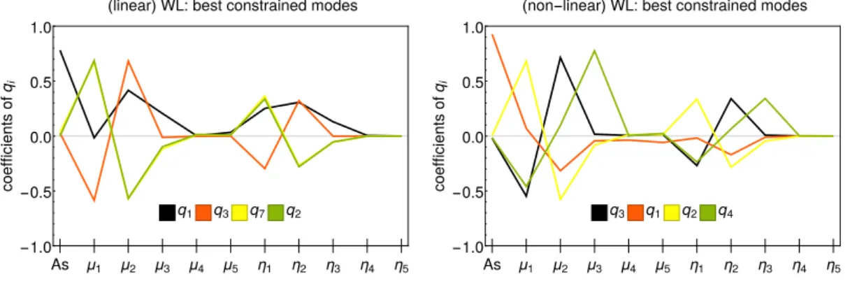
More generally, as we did for the GC case in the previous section, we look for theqi parameters with the smallest relative errors (σqi/qi) and find in the linear WL case, that the best constrained combinations (ordered from most to
least constrained) of primary parameters are given approximately by:
q1= +0.76`As+ 0.48µ2+ 0.33η2
q3=−0.59µ1+ 0.67µ2−0.30η1+ 0.32η2 q7= +0.65µ1−0.60µ2+ 0.36η1−0.28η2
q2= +0.67µ1−0.59µ2+ 0.33η1−0.29η2 .
(40)
This means that WL in the linear case will only be able to constrain combinations of the first two redshift bins in µ andη (corresponding to0. < z <1.0). This can also be observed graphically in the left panel of Figure 11. For the non-linear WL case, the combinations remain practically the same, except forq1, which will depend much more strongly on the parameter `As. The best 4 constrained parameters in this case, are (ordered from most to least
constrained):
q3=−0.55µ1+ 0.71µ2+−0.27η1+ 0.34η2
q1= +0.93`As−0.32µ2
q2= +0.67µ1−0.60µ2+ 0.33η1−0.29η2
q4=−0.46µ1+ 0.29µ2+ 0.73µ3+ 0.31η3 .
(41)
These combinations can also be visualized in the right panel of Figure 11. The complete matrixW of coefficients relating theqi to thepi parameters, can be found in Tables11and12of AppendixD.
q1 q3 q7 q2
As μ1 μ2 μ3 μ4 μ5 η1 η2 η3 η4 η5 -1.0
-0.5 0.0 0.5 1.0
coefficients
of
qi
(linear)WL: best constrained modes
q3 q1 q2 q4
As μ1 μ2 μ3 μ4 μ5 η1 η2 η3 η4 η5 -1.0
-0.5 0.0 0.5 1.0
coefficients
of
qi
(non-linear)WL: best constrained modes
Figure 11. Best constrained modes for a Euclid Redbook WL survey, with µand η binned in redshift, after transforming into uncorrelated q parameters via ZCA. Each of the four best constrained parameters qi, shown in the panels, is a linear combination of the primary parameterspi. qi in the label are ordered from the best constrained to the least constrained.
3. ZCA for Weak Lensing + Galaxy Clustering + CMB Planck priors