MNRAS-2016-Kuhn-4281-98.pdf

(1)

Advance Access publication 2016 April 15

KELT-10b: the first transiting exoplanet from the KELT-South survey – a

hot sub-Jupiter transiting a

V

=

10.7 early G-star

Rudolf B. Kuhn,

1‹

Joseph E. Rodriguez,

2‹

Karen A. Collins,

2,3

Michael B. Lund,

2

Robert J. Siverd,

4

Knicole D. Col´on,

5,6,7

Joshua Pepper,

5‹

Keivan G. Stassun,

2,8

Phillip A. Cargile,

9

David J. James,

10

Kaloyan Penev,

11

George Zhou,

12

Daniel Bayliss,

13,14

T. G. Tan,

15

Ivan A. Curtis,

16

Stephane Udry,

13

Damien Segransan,

13

Dimitri Mawet,

17,18

Saurav Dhital,

19

Jack Soutter,

20

Rhodes Hart,

20

Brad Carter,

20

B. Scott Gaudi,

21

Gordon Myers,

22,23

Thomas G. Beatty,

24,25

Jason D. Eastman,

9

Daniel E. Reichart,

26

Joshua B. Haislip,

26

John Kielkopf,

3

Allyson Bieryla,

9

David W. Latham,

9

Eric L. N. Jensen,

27

Thomas E. Oberst

28

and Daniel J. Stevens

21 Affiliations are listed at the end of the paper

Accepted 2016 April 12. Received 2016 March 8; in original form 2015 September 8

A B S T R A C T

We report the discovery of KELT-10b, the first transiting exoplanet discovered using the KELT-South telescope. KELT-10b is a highly inflated sub-Jupiter mass planet transiting a relatively bright V = 10.7 star (TYC 8378-64-1), with Teff = 5948 ± 74 K, logg =

4.319+₋0₀_..₀₃₀020and [Fe/H]=0.09₋+₀0_..11₁₀, an inferred massM_∗=1.112₋+₀0._.055₀₆₁Mand radiusR_∗= 1.209+₋0₀_..₀₃₅047R. The planet has a radiusRp=1.399₋+00..069049RJand massMp=0.679+₋00..039038MJ.

The planet has an eccentricity consistent with zero and a semimajor axisa=0.052 50+₋0₀..000 86000 97

au. The best-fitting linear ephemeris isT0=2457 066.720 45±0.000 27 BJDTDBandP=

4.166 2739±0.000 0063 d. This planet joins a group of highly inflated transiting exoplanets with a larger radius and smaller mass than that of Jupiter. The planet, which boasts deep transits of 1.4 per cent, has a relatively high equilibrium temperature ofTeq=1377+₋2823 K,

assum-ing zero albedo and perfect heat redistribution. KELT-10b receives an estimated insolation of 0.817+₋0₀..054068×109erg s−1cm−2, which places it far above the insolation threshold above which

hot Jupiters exhibit increasing amounts of radius inflation. Evolutionary analysis of the host star suggests that KELT-10b may not survive beyond the current subgiant phase, depending on the rate of in-spiral of the planet over the next few Gyr. The planet transits a relatively bright star and exhibits the third largest transit depth of all transiting exoplanets withV<11 in the Southern hemisphere, making it a promising candidate for future atmospheric characterization studies.

Key words: techniques: photometric – techniques: radial velocities – techniques: spectro-scopic – stars: individual: KELT-10 – planetary systems.

1 I N T R O D U C T I O N

Ground-based searches for transiting exoplanets have to date found more than 150 exoplanets (Schneider et al.2011).1 _Small aper-ture, wide-field robotic telescopes used by survey groups like

_E-mail: _{[email protected]} _(RBK); _{[email protected]} _(JER); [email protected](JP)

1_{http://exoplanet.eu/}

Net and HATSouth (Bakos et al. 2004, 2013), SuperWASP and WASP-South (Pollacco et al.2006; Hellier et al.2011), XO (Mc-Cullough et al.2005) and TrES (Alonso et al.2004) have been the most successful at finding exoplanets. Even with the suc-cess of these surveys, fewer than 25 transiting exoplanets with V < 11 have been discovered from the Southern hemisphere. Planets transiting bright stars are potentially the most scientifi-cally valuable, as these systems provide the opportunity to de-termine many precise properties of the planet itself (see Winn 2009).

2016 The Authors

at California Institute of Technology on September 9, 2016

http://mnras.oxfordjournals.org/

(2)

To illustrate this point, consider the transiting planet HD209458b (Charbonneau et al.2000; Henry et al.2000). With a magnitude ofV=7.95, this is one of the brightest transiting planet host stars and thus one of the best studied exoplanets. To date, over 50 pa-pers on various properties of the exoplanet2_{have been published.} Currently HD219134b (Motalebi et al. 2015) is the nearest and brightest host star with a known transiting exoplanet. This system shows enormous promise for future follow-up observations, which would better constrain the system architecture and characterize the physical properties of the planet.

More information can be gathered from bright transiting exoplan-ets due to the greater amount of flux from the host stars, enabling high-precision follow-up and characterization. It is for this specific reason the Transiting Exoplanet Survey Satellite (TESS; Ricker et al.2015) will perform a wide-field survey for planets that transit bright host stars. The TESS team expects to find∼1700 transiting exoplanets in the lifetime of the mission (Sullivan et al.2015) and a large fraction of TESS discovered planets will be attractive targets for follow-up measurements and atmospheric characterization due to their brightness.

The Kilodegree Extremely Little Telescope-South (KELT-South) transit survey (Pepper et al.2012) was built to detect giant, short-period transiting planets orbiting bright stars. The magnitude range 8<V<10 was selected (Pepper, Gould & Depoy2003) since most RV surveys target stars brighter thanV=9 and most transit surveys saturate for stars brighter thanV=10. Although the original speci-fication was forV<10, the KELT telescopes are capable of finding exoplanets around fainter stars and the first of the KELT telescopes, KELT-North (Pepper et al.2007), has already had success in finding brown dwarfs and planets around a large magnitude range of stars. KELT-1b (Siverd et al.2012) is a 27MJbrown dwarf transiting a V+10.7 F-star, with KELT-1 being the brightest star known to host a transiting brown dwarf. KELT-2Ab (Beatty et al.2012) is a hot Jupiter transiting the brightV+8.77 primary star in a visual binary system. KELT-3b (Pepper et al.2013) is a hot Jupiter transiting a V+9.8 slightly evolved late F-star. KELT-4Ab (Eastman et al.2016) is an inflated hot Jupiter transiting the brightest component in a V = 9.98 hierarchical triple. KELT-6b (Collins et al.2014) is a mildly inflated Saturn-mass planet transiting a metal poor, slightly evolvedV = 10.38 late F-star. KELT-7b (Bieryla et al.2015) is a hot Jupiter transiting a brightV =8.54 rapidly rotating F-star. KELT-8b (Fulton et al.2015) is a highly inflated hot Jupiter, with Rp=1.86₋+00..1816RJ, transiting a relatively brightV=10.83 G-star. This makes KELT-8b one of the best candidates for atmospheric characterization with transmission spectroscopy.

In this paper we describe the discovery and properties of KELT-10b, a hot sub-Jupiter (planets with radii similar to Jupiter and mass less than Jupiter) transiting the relatively bright V= 10.7 early G-star TYC 8378-64-1, the first exoplanet discovered by the KELT-South survey.

2 T H E K E LT- S O U T H S U RV E Y

Because this is the first paper describing an exoplanet discovery from the KELT-South survey, we describe the telescope instrumen-tation and observing site, survey strategy, data reduction method-ology, data reduction pipeline, light curve combination and

candi-2_See_{http://exoplanet.eu/catalog/hd_209458_b/}_{for a complete list of all}

publications.

date exoplanet selection criteria in detail. Additional information is available in section 2 of Siverd et al. (2012).

2.1 KELT-South instrumentation and observing site

Although the KELT-South instrumentation paper (Pepper et al. 2012) describes the KELT-South hardware in detail, there have been a number of small improvements and reconfigurations since that publication. In this section we summarize the current KELT-South hardware and computational setup and provide some basic performance metrics.

The KELT-South telescope consists of three main parts; camera and lens, mount, and control computer. The KELT-South detector is an Apogee Instruments Alta U16M thermo-electrically cooled CCD camera. The camera uses the Kodak KAF-16803 front illu-minated CCD with 4096×4096 9µm pixels (36.88×36.88 mm detector area) and has a peak quantum efficiency of∼60 per cent at 550 nm. The device is read out at 16 bit resolution at 1 MHz, giving a full-frame readout time of∼30 s. The CCD camera is maintained at−20◦C to reduce random thermal noise. The typical system noise for the CCD is given by the manufacturer as∼9e−at 1 MHz readout speed. In laboratory testing the nominal dark cur-rent was<1.4 e−pixel−1_s−1_{at a temperature of}₋₂₀◦_{C and the} CCD has temperature stability of±0.1◦C. The CCD operates at a conversion gain of 1.4e−ADU−1_{and the full-well depth is listed as}

∼100 000 e−, but the analogue-to-digital converter (ADC) saturates at 65535 ADU (∼92 000e−). The linear dynamic range is listed as 80 dB and the photoresponse non-linearity and non-uniformity are given as 1 per cent. The CCD also has anti-blooming protection to prevent image bleed from overexposed regions.

KELT-South uses a Mamiya 645 80 mm f/1.9 medium-format manual focus lens with a 42 mm aperture. The field of view using this lens is 26 deg×26 deg and provides∼23 arcsec pixel−1_image scale. In front of the lens is a Kodak Wratten No. 8 red-pass filter. This filter has a 50 per cent transmission point at∼490 nm. All the optical components are mounted on a Paramount ME Robotic Telescope mount manufactured by Software Bisque. The Paramount ME is a research-grade German Equatorial Mount design and has a tracking error of ±5 arcsec. The telescope needs to perform a meridian flip when taking images for fields crossing the meridian due to the way in which the camera and lens are attached to the mount.

The Dell Optiplex 755 small-form-factor computer that controls all aspects of the telescope operation runs the Windows XP op-erating system and is housed in a temperature controlled cabinet manufactured by Rittal. The Rittal cabinet also houses the UPS (uninterruptible power supply) unit to protect the computer against voltage spikes and brief power outages. The software packages (TheSky 6 Professional,CCDSOFTandTPOINT) provided by Software Bisque enable the control computer to operate the CCD and mount via a script-accessible interface. Various scripts, written in Visual Basic Scripting Edition, are used to perform the observing pro-cedures, basic image analysis to eliminate bad images, and data archiving.

The telescope is located at the South African Astronomical Ob-servatory site (20◦3848 E, 32◦2246 S, altitude 1768 m) near Sutherland, South Africa. Wind speeds less than 45 km s−1_occur 90 per cent of the time throughout the year and the median relative humidity level is 45 per cent (includes day and night time).

The point-spread function (PSF) of a star is dependent on the position of the star on the KELT-South CCD sensor and is charac-terized by a full width at half-maximum (FWHM) value of between

(3)

3 and 6 pixels. The KELT-South telescope operates slightly defo-cused to avoid undersampling of the stars. The telescope focus is not adjusted on a nightly basis and is kept at a fixed position through-out the lifetime of the telescope. Strict photometric conditions are required for optimal photometry, but a benefit of the large pixel scale of KELT-South is that large atmospheric seeing variations do not affect our ability to observe and good seeing conditions are not necessary for 10 mmag precision photometry for the brightest stars in the KELT-South survey.

2.2 Survey strategy

In the regular survey mode the telescope observes a number of fields located around the sky throughout the night. At present there are 29 fields observed in the survey schedule, which cover∼50 per cent of the southern sky. Survey observations consist of 150 s exposures with a typical per-field cadence of 15–30 min. KELT-South has been collecting survey data since 2010 February and to date has acquired between 2000 and 9000 images per field. Given this quantity of data and the typical achieved photometric precision of∼1 per cent for all stars withV≤11, the KELT-South survey is able to detect short-period giant transiting exoplanets orbiting most FGK dwarf stars with magnitudes from saturation nearV∼8 down toV∼11.

2.3 Data reduction

When constructing a data reduction pipeline, there are generally three options; aperture photometry, PSF fitting photometry, and im-age subtraction. Although aperture photometry and PSF photom-etry have been in use for an extended period of time and both of these reduction techniques are very well tested, KELT-South uses an image subtraction technique, first proposed by Tomaney & Crotts (1996). Image subtraction has been shown to work much better than aperture/PSF photometry at finding variable stars and transit-ing exoplanets in extremely crowded fields like globular clusters (Olech et al.1999; Hartman et al.2008; McCormac et al.2014) and open clusters (Hartman et al.2004; Howell et al.2005; Montalto et al.2007). The KELT-South telescope has an extremely wide field of view and large pixel scale, which necessitated the choice of an image subtraction data reduction pipeline over the other options.

South shares a data reduction pipeline with the KELT-North telescope (Pepper et al.2003; Gaudi et al.2015). Both tele-scopes use similar optics, with the only difference between the telescopes being the detector and minor differences in the observ-ing procedures. It is thus easy to use the same pipeline and reduction procedures for both telescopes with minor changes to accommodate these differences. KELT-South uses a slightly updated version of the pipeline, with new routines that are able to identify more individ-ual stars in extremely crowded regions. Additional information is available in Siverd et al. (2012) and Pepper et al. (2012).

2.4 Pipeline overview

The KELT project makes use of a heavily modifiedISIS3 difference-image-analysis package (Alard & Lupton 1998; Alard 2000; Hartman et al.2004) to achieve high-precision relative photome-try. Raw data images are dark-subtracted and flat-fielded. A master dark image is acquired by median combination of hundreds of dark images taken at the start of the observing season. This dark frame

3_See_{http://www2.iap.fr/users/alard/package.html}

is used for all data reduction and is infrequently updated. The data reduction pipeline is able to use a master dark image in this manner as we have found that the Poisson noise due to the bright back-ground sky is much larger than the systematic errors introduced by using an outdated dark image. A master flat-field image is used for all science images, which was constructed using hundreds of twilight sky flats, each of which was individually bias-subtracted, scaled-dark-subtracted, and additionally gradient-corrected prior to combination.

Light curves for individual objects are then constructed using the heavily modifiedISISimage-subtraction pipeline. Image subtraction is highly computer intensive. To improve performance theISISscripts were modified to facilitate distributed image reduction across many computers in parallel. Other elements of theISISpackage were also modified or replaced with faster alternatives. For example, the stan-dardISISsource-identification routines are ill equipped to deal with the nature and ubiquity of the aberrations in KELT-South images and theEXTRACTutility was replaced with the SEXTRACTORprogram (Bertin & Arnouts1996). More details of these modifications can be found online.4

Each observational image is examined for pointing scatter and a suitable high-quality image is selected to serve as an astromet-ric reference for that field. All the other images of that field are then registered (aligned) to this image. Shifts inxandypositions of the individual images are caused by incorrect pointing of the telescope or slight drifts due to an incorrect pointing model. Once all the images are registered, we median-combine all images, and create a list of all images that had a large number of pixels with outlying values from the median. We then median-combine again all images not on this list, and repeat the process of culling images two more times until the final median image is based on just the high-quality images. The highest quality images used to construct the master reference image are typically (a) acquired at low air mass, and (b) have low sky background flux. The result of this process is a maximally high signal-to-noise ratio (SNR) image that we use to define positions and fluxes of all objects identified for extraction.

The reference image is convolved using a series of Gaussian functions to match the object shapes and fluxes for each individual image, and the convolved reference is then subtracted from that image. By first matching object shapes in this fashion, we ensure that any residual flux has the same shape (PSF) as the original image. The residual flux from the subtracted image is then measured using PSF-weighted aperture photometry and added to the median flux of the object identified on the reference image. Median fluxes are obtained from the reference image using the stand-aloneDAOPHOT II (Stetson1987,1990). This allows us to assemble light curves for each individual object. Light curves are generated over the total baseline of the observations, rather than in separate time segments such as per night or per week.

2.5 Light curve combination and astrometry

The meridian flip of the telescope (see Section 2.1) causes images taken west of the meridian to be rotated by 180◦compared to im-ages taken east of the meridian. It is thus necessary to treat imim-ages taken on either side of the meridian as completely separate obser-vations. Because the telescope optics are not exactly axisymmetric, the PSFs of stars in the corners of the field of view are not ex-actly the same in each orientation, and different reference images

4_{http://astro.phy.vanderbilt.edu/~siverdrj/soft/is3/index.html}

(4)

for the eastern and western orientations were created to account for the non-symmetrical nature of the distortions. Other factors like flat fielding errors and detector defects also contribute to images obtained in either orientation being slightly different. The data re-duction pipeline produces two versions of a light curve for each identified object in each orientation. The first is the raw flux con-verted, 3σ clipped light curve that removes all outlier data points. We call this the ‘processed light curve’. The second version of the light curve is a trend filtered light curve. A 90 d median smoothing is applied to remove long-term trends before we use the Trend Fil-tering Algorithm (TFA; Kov´acs, Bakos & Noyes2005) to remove common systematics in the light curves. We use the closest 150 neighbouring stars that are within three instrumental magnitudes as an input template to detrend the light curve for each star. This detrended light curve is called the ‘TFA light curve’.

We use theASTROMETRY.NETpackage (Lang et al.2010) to find as-trometric solutions for each of our reference images (east and west reference image separately).ASTROMETRY.NETperforms astrometric image calibrations without any prior input aside from the data in the image pixels themselves. The calibration information thatASTROM -ETRY.NETprovides includes image pointing, orientation, plate scale and full coordinate solutions.

To get a combined light curve for each star, KELT-South objects from the eastern and western reference images are first matched to objects listed in the Tycho-2 catalogue (Høg et al.2000) separately. KELT-South objects are matched to Tycho-2 objects if the sky pro-jected distance between them is less than 76 arcsec (∼3.5 pixels). We chose this distance as it produced the fewest number of double matches (i.e. when more than one KELT-South object is matched to the same Tycho-2 object), while still producing a relatively large fraction of correctly matched stars. If more than one match was found for a Tycho-2 star in the reference image, we selected the closest KELT-South object as the matching object (unless the mag-nitude difference indicated a wrong match). Using the Tycho-2 po-sitional information for each KELT-South object, we match the Tycho-2 objects to objects in the UCAC4 catalogue (Zacharias et al. 2013). Finally the eastern and western median-subtracted light curves (matched using the Tycho-2 IDs) are combined and the median magnitude is used as the final KELT-South instrumental magnitude.

At the end of the data reduction process, we thus have a final total of two light curves for each object identified, one combined processed light curve and one combined TFA light curve.

2.6 Candidate selection

We present a summary of the KELT-South candidate selection pro-cess, which involves a number of procedures, and emphasize the modifications from the steps followed in the discovery paper of KELT-1b (Siverd et al. 2012) from the KELT-North survey. The matching of the object to Tycho-2 and UCAC4 simultaneously provides proper motions and B, V,J, H, andK apparent magni-tudes. Next, giant stars are identified and excluded from our sam-ple using a reduced proper motion cut (Gould, Pepper & DePoy 2003) following the procedure outlined by Collier Cameron et al. (2007), with the slight modifications shown in equations 1 and 2 in section 2.3 of Siverd et al. (2012).

For most KELT-South fields, the combined light curves use the eastern orientation ID; however, the KELT-South field 27 (KELT-10b’s location) and 28 combined light curves were the first fields processed and were given a unique internal ID in a process similar to that of KELT-North. Using the box-least-squares (BLS) algorithm

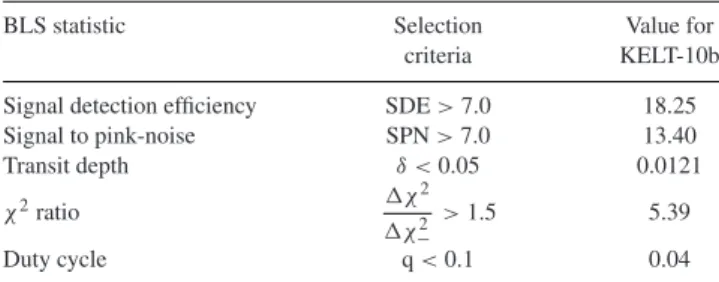
Table 1. KELT-South BLS selection criteria for candidate exoplanet light curves and values for KELT-10b.

BLS statistic Selection Value for

criteria KELT-10b

Signal detection efficiency SDE>7.0 18.25

Signal to pink-noise SPN>7.0 13.40

Transit depth δ <0.05 0.0121

χ2_ratio χ

2

χ2

−

>1.5 5.39

Duty cycle q<0.1 0.04

(Kov´acs, Zucker & Mazeh2002), we search the combined light curves for periodic transit signals. The selection cuts are performed on five of the statistics output by theVARTOOLS (Hartman2012) implementation of the BLS algorithm. The selection criteria we use are the same as presented in Siverd et al. (2012) and are shown in Table1(Kov´acs et al.2002; Burke et al.2006; Hartman et al. 2008). Finally, we apply the same stellar density cut as shown in equations 4 and 5 of section 2.3 of Siverd et al. (2012) but do not apply theTeff cut of <7500 K. All targets that pass the cuts described here are assigned as candidates and a web page is created containing all the information from the analysis above, along with additional diagnostic tests based on the Lomb–Scargle (LS; Lomb1976; Scargle 1982) and analysis-of-variance (AoV; Schwarzenberg-Czerny1989; Devor2005) algorithms.

From this analysis, we typically find anywhere from 100 to 1500 candidates per KELT-South field (depending on the proximity of the field to the Galactic plane). The KELT-South team individually votes on each candidate in a field and designates each as either a planet or a false positive (such as an eclipsing binary or spurious detection). All candidates with one or more votes for planet are then discussed. From the discussion, the most promising potential planet candidates are sent for follow-up photometric confirmation, reconnaissance spectroscopy, or in very promising cases, both.

3 D I S C OV E RY A N D F O L L OW- U P O B S E RVAT I O N S

3.1 KELT-South observations and photometry

KELT-10b is located in the KELT-South field 27 with field centre located at J2000α=19h₅₅m₄₈s_and_δ_{= −}₅₃◦₀₀₀₀_{. Field 27 was} monitored fromUT2010 March 19 toUT2014 April 18 with over 5000 images acquired during that time (4967 observations were used in the final light curve). We reduced the raw survey data using the pipeline described in Section 2 and performed candidate vetting and selection as described in Section 2.6. One of the candidates from field 27 (KS27C013526) was star TYC 8378-64-1/2MASS 18581160-4700116, located at J2000α=18h₅₈m₁₁s_._{601 and}_δ₌

−47◦0011.68. The star has Tycho magnitudesBT =11.504 and

VT=10.698 (Høg et al.2000). Full catalogue properties of this star

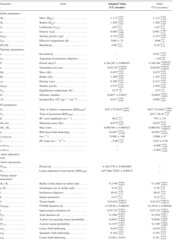
are provided in Table2. The light curve of KS27C013526 has a weighted RMS of 11.9 milli-magnitudes (mmag), which is typical for KELT-South light curves with magnitude around V= 11. A significant BLS signal was found at a period of P 4.1664 439 d, with a transit depth ofδ 12.1 mmag. Further detection statistics are listed in Table1. The discovery light curve of KELT-10b is shown in Fig.1.

(5)

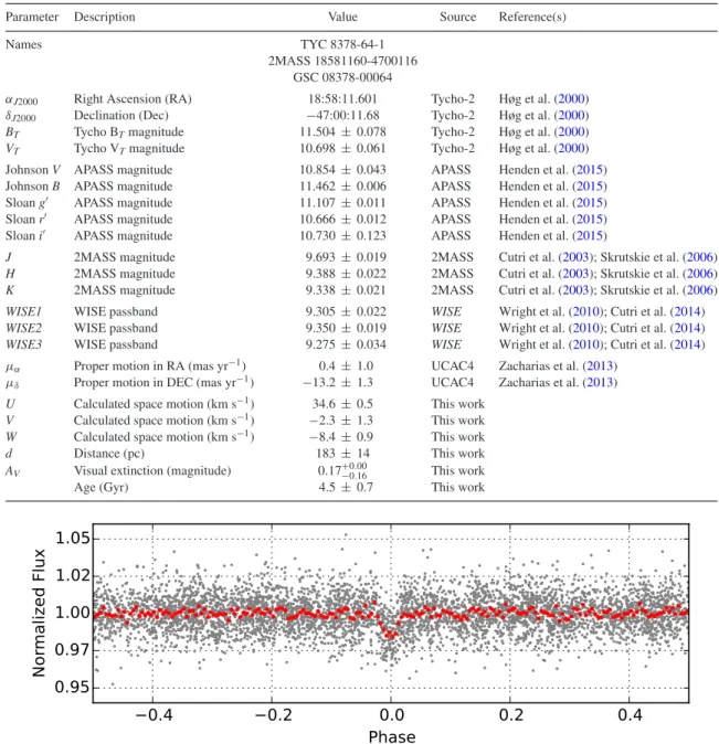
Table 2. Stellar properties of KELT-10 obtained from the literature.

Parameter Description Value Source Reference(s)

Names TYC 8378-64-1

2MASS 18581160-4700116 GSC 08378-00064

αJ2000 Right Ascension (RA) 18:58:11.601 Tycho-2 Høg et al. (2000)

δJ2000 Declination (Dec) −47:00:11.68 Tycho-2 Høg et al. (2000)

BT Tycho BTmagnitude 11.504±0.078 Tycho-2 Høg et al. (2000)

VT Tycho VTmagnitude 10.698±0.061 Tycho-2 Høg et al. (2000) JohnsonV APASS magnitude 10.854±0.043 APASS Henden et al. (2015) JohnsonB APASS magnitude 11.462±0.006 APASS Henden et al. (2015) Sloang APASS magnitude 11.107±0.011 APASS Henden et al. (2015) Sloanr APASS magnitude 10.666±0.012 APASS Henden et al. (2015) Sloani APASS magnitude 10.730±0.123 APASS Henden et al. (2015)

J 2MASS magnitude 9.693±0.019 2MASS Cutri et al. (2003); Skrutskie et al. (2006)

H 2MASS magnitude 9.388±0.022 2MASS Cutri et al. (2003); Skrutskie et al. (2006)

K 2MASS magnitude 9.338±0.021 2MASS Cutri et al. (2003); Skrutskie et al. (2006)

WISE1 WISE passband 9.305±0.022 WISE Wright et al. (2010); Cutri et al. (2014)

WISE2 WISE passband 9.350±0.019 WISE Wright et al. (2010); Cutri et al. (2014)

WISE3 WISE passband 9.275±0.034 WISE Wright et al. (2010); Cutri et al. (2014) μα Proper motion in RA (mas yr−1) 0.4±1.0 UCAC4 Zacharias et al. (2013)

μδ Proper motion in DEC (mas yr−1₎ ₋_13.2_±_1.3 _UCAC4 _{Zacharias et al. (}₂₀₁₃₎

U Calculated space motion (km s−1₎ _34.6_±_0.5 _{This work}

V Calculated space motion (km s−1₎ ₋_2.3_±_1.3 _{This work}

W Calculated space motion (km s−1₎ ₋_8.4_±_0.9 _{This work}

d Distance (pc) 183±14 This work

AV Visual extinction (magnitude) 0.17+₋00..0016 This work

Age (Gyr) 4.5±0.7 This work

Figure 1. Discovery light curve of KELT-10b from the KELT-South telescope. The light curve contains 4967 observations spanning just over 4 yr, phase folded to the orbital period of P=4.166 4439 d. The red points show the light curve binned in phase using a bin size of 0.005 (≈30 min). These points are shown for illustrative purposes only and are not used in the final global fit described in Section 5.1. [A colour version of this figure is available in the online journal. A table containing all the KELT-South measurements is available in a machine-readable form in the online journal.]

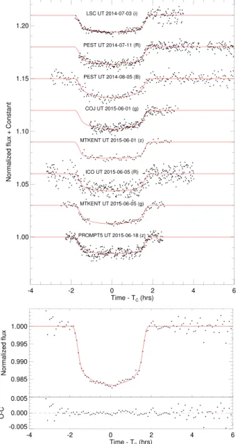
3.2 Follow-up photometry

We obtained follow-up time series photometry of KELT-10b to check for false positives, better determine the transit shape, and better determine the phase and period of the transiting exoplanet. We used theTAPIRsoftware package (Jensen2013) to predict transit events, and we obtained eight full or partial transits in multiple bands between 2014 July and 2015 June. All data were calibrated and processed using the AstroImageJ package (AIJ)5 (Collins & Kielkopf2013; Collins, Kielkopf & Stassun2016) unless otherwise stated. For all follow-up photometric observations, we use theAIJ package to determine the best detrending parameters to include in

5_{http://www.astro.louisville.edu/software/astroimagej}

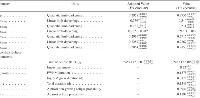
the global fit. Table3lists the follow-up photometric observations and the detrending parameters determined by AIJ. All follow-up photometry is shown in Fig.2.

3.2.1 LCOGT observations

The Las Cumbres Observatory Global Telescope (LCOGT) network6 _{consists of a globally distributed set of telescopes. We} observed a nearly full transit of KELT-10b in the Sloani-band on UT2014 July 03 from a LCOGT 1 m telescope at Cerro Tololo Inter-American Observatory (CTIO), with a 4K × 4K Sinistro

6_{http://lcogt.net/}

(6)

Table 3. Photometric follow-up observations and the detrending parameters found byAIJfor the global fit.

Follow-up observations Date (UT) Filter Detrending parameters used in the global fit

LCOGT 2014 July 3 i airmass

PEST 2014 July 11 R time, FWHM,xycoordinates

PEST 2014 August 5 B sky counts,xycoordinates

LCOGT 2015 June 1 g airmass, total counts

Adelaide 2015 June 1 R airmass, sky counts, total counts

Mt Kent 2015 June 1 z airmass, FWHM, sky counts

Mt Kent 2015 June 5 g airmass, total counts

Skynet 2015 June 18 z airmass, meridian flip, FWHM, total counts

Notes.The tables for all the follow-up photometry are available in machine-readable form in the online journal.

detector with a 27 arcmin×27 arcmin field of view and a pixel scale of 0.39 arcsec pixel−1_{, labelled as ‘LSC’ in Fig.}₂_{. We also} observed a partial transit in the Sloan g-band onUT2015 June 01 from a 1 m LCOGT telescope at Siding Springs Observatory SSO, labelled as ‘COJ’ in Fig.2, with a 4K×4K SBIG Science camera with a 16 arcsec×16 arcsec field of view and a pixel scale of 0.23 arcsec pixel−1_{. The reduced data were downloaded from} the LCOGT archive and observations were analysed using custom routines written in GDL.7

3.2.2 Skynet observations

The Skynet network (Reichart et al.2005)8_{is another set of} dis-tributed telescopes. We observed a partial transit of KELT-10b in the Sloanz-band onUT2015 June 18 from CTIO using the 0.4 m Prompt5 telescope from the PROMPT (Panchromatic Robotic Op-tical Monitoring and Polarimetry Telescope) subset of Skynet tele-scopes. The Prompt5 telescope hosts an Alta U47+s camera by Apogee, which has an E2V 1024×1024 CCD, a field of view of 10 arcmin×10 arcmin, and a pixel scale of 0.59 arcsec pixel−1_. Re-duced data were downloaded from the Skynet website and analysed using custom GDL routines.

3.2.3 PEST observations

The PEST (Perth Exoplanet Survey Telescope) observatory is a backyard observatory owned and operated by Thiam–Guan (TG) Tan. It is equipped with a 12 inch Meade LX200 SCT f/10 tele-scope with focal reducer yielding f/5. The camera is an SBIG ST-8XME, and focusing is computer controlled with an Optec TCF-Si focuser. CCD Commander is used to script observations, FocusMax for focuser control, and CCDSoft for control of the CCD camera. PinPoint is used for plate solving. A partial transit (covering the last half of ingress to almost 2 h after egress) was observed inRonUT 2014 July 11. A full transit inBwas observed onUT2014 August 5.

3.2.4 Adelaide observations

The Adelaide Observatory owned and operated by Ivan Curtis is largely run manually from his back yard in Adelaide, South Aus-tralia. The observatory is equipped with a 9.25 inch Celestron SCT telescope with an Antares 0.63×focal reducer yielding an over-all focal ratio of f/6.3. The camera is an Atik 320e, which uses a

7_{GNU Data Language;}_{http://gnudatalanguage.sourceforge.net/} 8_{https://skynet.unc.edu/}

cooled Sony ICX274 CCD of 1620×1220 pixels. The field of view is∼16.6 arcmin×12.3 arcmin with a resolution of 0.62 arc-sec pixel−1_{. We observed a complete transit of KELT-10b in}_R_on UT2015 June 5 (see light curve ‘ICO’ in Fig.2).

3.2.5 Mt Kent observations

A partial transit of KELT-10b was observed in the Sloanz-band on UT2015 June 1 and a full transit was observed in the Sloang-band onUT2015 June 5 (see Fig.2) from the Mt Kent Observatory, located outside Toowoomba, Queensland, Australia. All observations were performed with a defocused 0.5 m Planewave CDK20 telescope equipped with an Alta U16M Apogee camera. This combination produces a 36.7 arcmin×36.7 arcmin field of view and a pixel scale of 0.5375 arcsec pixel−1_{. Conditions on both nights were} clear, however both observations were taken close to full Moon.

3.3 Spectroscopic follow-up

3.3.1 Spectroscopic reconnaissance

In order to rule out eclipsing binaries and other common causes of false positives for transiting exoplanets surveys, we acquire spec-tra of KELT-South candidates using the Wide Field Spectrograph (WiFeS; Dopita et al.2007) on the Australian National University (ANU) 2.3 m telescope at Siding Spring Observatory in Australia. We follow the observing methodology and data reduction pipeline as set out in Bayliss et al. (2013). A single 100 s spectrum of KELT-10 was obtained using the B3000 grating of WiFeS on 2014 July 9, which delivers a spectrum ofR =3000 from 3500 Å to 6000 Å. From this spectrum we determined KELT-10 to be a dwarf star with an effective temperature of 6100±100 K. We then ob-tained four higher resolution spectra (with exposure times of∼60 s), spanning the nights 2014 July 9 to 2014 July 11, with the R7000 grating of WiFeS. This grating delivers a spectral resolution ofR =7000 across the wavelength region 5200–7000 Å, and provides radial velocities precise to the±1 km s−1_{level. From these four} measurements we determined that KELT-10 did not display any ra-dial velocity variations above the level ofK=1 km s−1_{, ruling out} eclipsing binaries with high amplitude radial velocity variations. The candidate was therefore deemed to be a high priority target for high-precision radial velocity follow-up (see Section 3.3.2).

To date we have vetted 105 KELT-South candidates using the WiFeS on the ANU 2.3 m telescope, of which 67 (62.6 per cent) have been ruled out as eclipsing binaries due to high-amplitude, in-phase, radial velocity variations. A further two candidates (1.9 per cent) were ruled out after they were identified as giants. Typically each KELT-South candidate requires only 5 min oftotalexposure time

(7)

Figure 2. Top: follow-up transit photometry of KELT-10. The labels are LSC=CTIO LCOGT observations (see Section 3.2.1, PEST=Perth Ex-oplanet Survey Telescope observations (see Section 3.2.3), COJ=SSO LCOGT observations (see Section 3.2.1), ICO=Adelaide Observatory (Ivan Curtis Observatory) observations (see Section 3.2.4), MTKENT=Mt Kent Observatory observations (see Section 3.2.5), and Prompt5=CTIO Skynet observations (see Section 3.2.2). Bottom: all the follow-up light curves combined and binned in 5 min intervals. This light curve is not used for analysis, but rather to show the best combined behaviour of the transit. The solid red line shows the transit model from the global fitting procedure described in Section 5.1 for each of the individual light curves. [A colour version of this figure is available in the online journal.]

for this vetting, making it an extremely efficient method of screening candidates compared to photometric follow-up or high-resolution spectroscopy.

3.3.2 High-precision spectroscopic follow-up

Multi-epoch, high resolution spectroscopy with a stabilized spec-trograph can provide high-precision radial velocity measurements capable of confirming the planetary nature of a transiting

exo-Table 4. KELT-10 radial velocity observations with CORALIE.

BJDTDB RV RV error

(m s−1₎ _{(m s}−1₎

2456937.517729 31 942.72 9.73

2456938.541050 31 836.89 10.06

2456942.492638 31 840.37 12.48

2456943.496229 31 886.32 10.97

2456944.494299 31 982.29 10.83

2456946.495001 31 861.65 15.14

2456948.521337 31 981.69 9.40

2456949.497177 31 971.14 11.19

2456950.523627 31 865.72 10.55

2456951.521526 31 852.24 9.39

2456953.505857 31 991.27 12.97

2456954.499325 31 887.12 11.57

Notes.This table is available in its entirety in a machine-readable form in the online journal.

Figure 3. CORALIE radial velocity measurements and residuals for KELT-10. The best-fitting model is shown in red. The bottom panel shows the residuals of the RV measurements to the best-fitting model. [A colour version of this figure is available in the online journal.]

planet candidate and precisely measuring its true mass. We obtained high-precision radial velocity measurements for KELT-10 using the CORALIE spectrograph (Queloz et al.2001a) on the Swiss 1.2 m Leonard Euler telescope at the ESO La Silla Observatory in Chile. CORALIE is a fibre-fed echelle spectrograph which provides sta-ble spectra with spectral resolution of R= 60 000. Spectra are taken with a simultaneous exposure of a Thorium–Argon discharge lamp acquired through a separate calibration fibre, which allows for radial velocities to be measured at levels better than 3 m s−1 for bright stars (Pepe et al.2002). Data are reduced and radial ve-locities computed in real time via the standard CORALIE pipeline, which cross-correlates the stellar spectra with a numerical mask with non-zero zones corresponding to stellar absorption features at zero velocity. Radial velocities were measured for KELT-10 over 12 different epochs between 2014 October 7 and 2014 October 23, spanning a range of orbital phases. The results are presented in Table4and Fig.3. The radial velocities displayed a sinusoidal vari-ation with a period and phase that matched the orbit as determined from the discovery and follow-up photometry. The peak-to-peak amplitude of the variation was 154 m s−1_{, indicative of a} short-period hot Jupiter (see Fig.4). Bisector spans were measured using the CCF peak as described in (Queloz et al.2001b) and no correla-tion is evident between the bisector spans and the radial velocities (see Fig. 5), helping rule out a blended eclipsing binary system (Gray1983,2005). These radial velocities are used in the global modelling of the KELT-10 system as set out in Section 5.1.

(8)

Figure 4. Radial velocity measurements phase-folded to the best-fitting linear ephemeris. The best-fitting model is shown in red. The predicted Rossiter–McLaughlin effect assumes perfect spin-orbit alignment and it is not well constrained by our data. The bottom panel shows the residuals of the RV measurements to the best-fitting model. [A colour version of this figure is available in the online journal.]

Figure 5. Bisector measurements for the CORALIE spectra used for radial velocity measurements. We find no significant correlation between RV and the bisector spans. [A colour version of this figure is available in the online journal.]

3.4 Adaptive optics observations

Adaptive optics (AO) imaging places limits on the existence of nearby eclipsing binaries that could be blended with the primary star KELT-10 at the resolution of the KELT-South and follow-up data, thereby causing a false-positive planet detection. In addition, it places limits on any nearby blended source that could contribute to the total flux, and thereby result in an underestimate of the transit depth and thus planet radius in the global fit presented in Section 5.1.

We observed KELT-10 with the Nasmyth Adaptive Optics Sys-tem (NAOS) Near-Infrared Imager and Spectrograph (CONICA) instrument (Lenzen et al. 2003; Rousset et al.2003) on the Very Large Telescope (VLT) located at the ESO Paranal observatory as

Figure 6. The NAOS-CONICA AO image of KELT-10. The location of KELT-10 is shown by the green cross. North is up, east is left. A horizontal 1 arcsec bar is also shown for scale. A faint companion (circled in green) withK=9±0.3 mag located 1.1 arcsec to the SE of KELT-10 is clearly visible. [A colour version of this figure is available in the online journal.]

part of the program 095.C-0272(A) ‘Adaptive Optics imaging of the Brightest Transiting Exoplanets from KELT-South’ (PI: Mawet) on UT2015 August 7. We used theKs-band filter and the S13 camera which has a plate scale of 0.013 arcsec pixel−1_.

The images were acquired as a sequence of 30 dithered exposures. Each exposure was the average of 10 frames with 6 s integration time, making for a total open shutter time of 1800 s. We used the pupil tracking mode where the instrument corotates with the tele-scope pupil to fix diffraction and speckles to the detector reference frame, allowing the sky to counter-rotate with the parallactic angle, effectively enabling angular differential imaging.

We reduced the data by subtracting a background image made out of median-combined dithered frames, dividing by a flat-field and in-terpolating for bad pixels and other cosmetics. The reduced images were then processed using principal component analysis (Soummer, Pueyo & Larkin2012) to mitigate speckle noise, yielding the image shown in Fig.6.

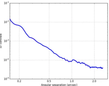
We calculate the 5σ contrast limit as a function of angular sepa-ration by defining a series of concentric annuli centred on the star. For each of the concentric annuli, we calculated the median and the standard deviation of flux for pixels within this annulus. We used the value of five times the standard deviation above the median as the 5σdetection limit. The resulting 5σcontrast curve is presented in Fig.7.

An off-axis point source with a contrast ofK=9±0.3 mag-nitude to the primary is detected at a distance of 1.1 arcsec ± 0.013 arcsec at position angle of 119◦. At a separation of 1.1 arc-sec, it is unclear whether or not the companion is bound to KELT-10. If the companion is bound, we calculate an absolute MK=12.026

at a distance of 183±14 pc (see Section 4.2). Using the Baraffe (Baraffe et al.2002) models we estimate a mass of 0.073 Mfor the companion, which is consistent with a very late-M dwarf star, just barely above the sub-stellar boundary.

Additional high-contrast follow-up imaging of the system could help determine whether or not the faint companion is bound, but the proper motion of KELT-10 is not very large. If the companion were a distant background source (thus∼stationary), it would separate from 10 with a speed comparable to proper motion of KELT-10. A 15-yr baseline in follow-up imaging would only provide a movement of 270 milli-arcsec, which necessitates highly accurate

(9)

Figure 7. 5σ detection limit as a function of angular separation derived from the NAOS-CONICA AO image around KELT-10. [A colour version of this figure is available in the online journal.]

astrometric and long-term monitoring to determine the physical association between the two stars.

To test the probability of chance alignment for the KELT-10 bi-nary system, we used an statistical model of the Galactic stellar distribution (Dhital et al.2010). A more detailed description of this analysis is shown in Dhital et al. (2010) but we provide a brief, pertinent description here. The Galactic model is parametrized by an empirically measured stellar number density distribution in a 30 arcmin×30 arcmin conical volume centred at Galactic position of KELT-10. The number density distributions are constrained by empirical measurements from the Sloan Digital Sky Survey (Juri´c et al.2008; Bochanski et al.2010) and accurately account for the decrease in stellar number density with both Galactocentric radius and Galactic height. Using the Galactic model to calculate the fre-quency of unrelated, random pairings within the volume defined by the KELT-10 binary, assuming that all the simulated stars are, by definition, single. Thus, any random pairing was flagged as a chance alignment. In 106 _{independent simulations, only 86} pro-duced a random pairing, equating to a chance alignment probability of 0.0086 per cent. This provides strong evidence that the neigh-bouring star is a bound companion to KELT-10A (TYC 8378-64-1).

4 H O S T S TA R P R O P E RT I E S

4.1 SME stellar analysis

In order to determine precise stellar parameters for KELT-10, we utilized the 12 high-resolution R ∼55 000, low S/N∼10–20 CORALIE spectra acquired for radial velocity confir-mation of KELT-10b. For each of the individual spectra, we contin-uum normalized each echelle order, stitched the orders into a single 1-D spectrum, and shifted the wavelengths to rest velocity by ac-counting for barycentric motion, the space velocity of KELT-10, as well as the radial velocity induced by KELT-10b. The 12 individual 1-D spectra were then co-added using the median of each wave-length resulting in a single spectrum with S/N∼30–50, sufficient for detailed spectroscopic analysis.

Stellar parameters for KELT-10 are determined using an imple-mentation of Spectroscopy Made Easy (SME; Valenti & Piskunov 1996). We base the general method of our SME analysis on that

given in Valenti & Fischer (2005); however, we use a line list, syn-thesized wavelength ranges, and abundance pattern adapted from Stempels et al. (2007) and Hebb et al. (2009), and also incorporate the newest MARCS model atmospheres (Gustafsson et al.2008). The details of our technique are outlined in the recent analysis of WASP-13 (G´omez Maqueo Chew et al.2013). Briefly, we have expanded on the technique outlined in Valenti & Fischer (2005) that allows us to operate SME in an automated fashion by utilizing massive computational resources. We have developed an exten-sive Monte Carlo approach to using SME by randomly selecting 500 initial parameter values from a multivariate normal distribution with five parameters: effective temperature (Teff), surface gravity (logg_∗), iron abundance ([Fe/H]), metal abundance ([m/H]), and rotational velocity of the star (vsinI_∗). We then allow SME to find a best-fitting synthetic spectrum and solve for the free parameters for the full distribution of initial guesses, producing 500 best-fitting so-lutions for the stellar parameters. We determine our final measured stellar properties by identifying the output parameters that give the optimal SME solution (i.e. the solution with the lowestχ2_{). The} overall SME measurement uncertainties in the final parameters are calculated by adding in quadrature: (1) the internal error determined from the 68.3 per cent confidence region in theχ2_{map, and (2) the} median absolute deviation of the parameters from the 500 output SME solutions to account for the correlation between the initial guess and the final fit.

Our final SME spectroscopic parameters for KELT-10 are: Teff= 5925±79 K (in good agreement with the independently determinedTefffound by the ANU analysis), logg∗=4.38±0.17, [m/H]=0.05±0.06, [Fe/H]=0.12±0.11 and a projected rota-tional velocityvsinI_∗<3.6 km s−1_{. We constrain the macro- and} microturbulent velocities to the empirically constrained relation-ship, similar to G´omez Maqueo Chew et al. (2013); however, we do allow them to change during our modelling according to the other stellar parameters. Our best-fitting stellar parameters result invmac

=4.14 km s−1_and_v

mic=1.05 km s−1. We note the large error bars on [Fe/H] are likely due to the relatively low S/N of the co-added CORALIE spectrum (estimated to be S/N∼30–50). Also, we find that we are unable to resolve the rotational velocity (vsinI∗) of KELT-10 from the instrument profile of CORALIE, likely due to the combination of the low S/N of the co-added spectrum and the star’s slow rotation. We therefore are only able to infer an upper limit ofvsinI∗<3.6 km s−1_.

4.2 Spectral energy distribution analysis

We construct an empirical spectral energy distribution (SED) of KELT-10 using all available broad-band photometry in the literature, shown in Fig.8. We use the near-UV flux fromGALEX(Martin et al. 2005), theBTandVTfluxes from the Tycho-2 catalogue,B,V,g,r,

andifluxes from the AAVSO APASS catalogue, NIR fluxes in the J,H, andKSbands from the 2MASS Point Source Catalogue (Cutri

et al.2003; Skrutskie et al.2006), and near-and mid-infrared fluxes in theWISEpassbands (Wright et al.2010).

We fit these fluxes using the Kurucz atmosphere models (Castelli & Kurucz2004) by fixing the values ofTeff, logg∗and [Fe/H] in-ferred from the global fit to the light curve and RV data as described in Section 5.1 and listed in Table4, and then finding the values of the visual extinctionAVand distancedthat minimizeχ2, with a

maxi-mum permittedAVof 0.17 based on the full line-of-sight extinction

from the dust maps of Schlegel, Finkbeiner & Davis (1998). We findAV =0.17+−00..0016 andd= 183± 14 pc with the best-fitting model having a reduced χ2 ₌ _{1.34. This implies a very}

(10)

Figure 8. Measured and best-fitting SED for KELT-10 from ultraviolet through mid-infrared. The red error bars indicate measurements of the flux of KELT-10 in ultraviolet, optical, near-infrared and mid-infrared passbands as listed in Table2. The vertical bars are the 1σphotometric uncertainties, whereas the horizontal error bars are the effective widths of the passbands. The solid curve is the best-fitting theoretical SED from the Kurucz mod-els (Castelli & Kurucz2004), assuming stellar parametersTeff, logg∗and [Fe/H] fixed at the adopted values in Table5, with AVanddallowed to vary. The blue dots are the predicted passband integrated fluxes of the best-fitting theoretical SED corresponding to our observed photometric bands. [A colour version of this figure is available in the online journal.]

good quality of fit and further corroborates the final derived stellar parameters for the KELT-10 host star. We note that the quoted statistical uncertainties on AVanddare likely to be underestimated

because we have not accounted for the uncertainties inTeff, logg∗ and [Fe/H] used to derive the model SED. Furthermore, it is likely that alternate model atmospheres would predict somewhat different SEDs and thus values of extinction and distance.

Nonetheless, the best-fitting SED model places the system at a vertical height of only∼60 pc, well within the local dust disc scale height of 125 pc (Marshall et al. 2006), and the system is seen through just over half of the local column of extinction.

4.3 UVW space motion

Determining of the three-dimensional velocity of an object as it passes through the Galaxy can help to assess its age and member-ship in stellar groups or associations, especially if it belongs to an identifiable kinematic stream. Following the procedures detailed in Johnson & Soderblom (1987), we calculate the UVW space motion of the KELT-10 system and examine its potential membership in known stellar groups or kinematic streams in the solar neighbour-hood.

Employing the KELT-10 astrometric and two-dimensional kine-matic data detailed in Table2, as well as its centre-of-massγ veloc-ity listed in Table5, only a precise and accurate distance is further required in order to calculate its UVW space motion. Because the KELT-10 system is too faint to have been observed by the Hippar-cosmission, its trigonometric parallax is not known and we use the distanced=183±14 derived from the SED analysis in Section 4.2. For the host star of KELT-10b, we calculate its space motions to beU=34.6±0.5 km s−1_,_V_{= −}_2.3_±_{1.3 km s}−1_and_W_{= −}_8.4_± 0.9 km s−1_{(with positive U pointing towards the Galactic Centre).} In the calculation of the UVW space motion, we have corrected for

the peculiar velocity of the Sun with respect to the local standard of rest (LSR) using the values ofU=8.5 km s−1_,_V₌_{13.38 km s}−1 andW=6.49 km s−1_{from Cos¸kuno˘glu et al. (}₂₀₁₁_).

In U–V space, KELT-10 is not consistent with the kinematics of young disc objects, nor with the Pleiades, Hyades, and Ursa Major groups (Montes et al.2001; Seifahrt et al.2010). In fact, the same lack of kinematic membership is also true of the AB Dor, Argus, Beta Pic, Carina, Columba, Tuc-Hor, TW Hya groups (Bowler et al. 2013). In V–W space however, KELT-10 is border-line consistent with the Beta Pic group (Bowler et al.2013) and the local young disc population (Seifahrt et al.2010). However, our age estimate for KELT-10 (4.5±0.7 Gyr) makes it unlikely to be a member of the young disc population.

We therefore posit that KELT-10’s UVW space motion does not place it among any of the local, young kinematic moving groups of stars, and its space motion appears unremarkable. The UVW space motion is consistent with a thin disc source at∼99 per cent probability, according to the criteria set out in Bensby, Feltzing & Lundstr¨om (2003).

4.4 Stellar models and age

To better place the KELT-10 system in context, we show in Fig.9the H–R diagram for KELT-10 in theTeffversus logg∗plane. We use the Yonsei–Yale stellar evolution model track (Demarque et al.2004) for a star with the mass and metallicity inferred from the global fit, where the shaded region represents the mass and [Fe/H] fit uncertainties. The model isochrone ages are indicated as blue points, and the final best global fitTeffand logg∗ values are represented by the red error bars. For comparison, theTeffand logg_∗values determined from spectroscopy alone are represented by the green error bars. KELT-10 is evidently a G0V star (Pickles & Depagne2010) with an apparent age of∼4.5±0.7 Gyr.

5 P L A N E TA RY P R O P E RT I E S

5.1 Global modelling with EXOFAST

Using a modified version of the IDL exoplanet fitting tool, EX -OFAST (Eastman, Gaudi & Agol 2013), we perform a global fit of both the photometric and spectroscopic data described in Sec-tions 3.1, 3.2 and 3.3. This process is described further in Siverd et al. (2012). Using the Yonsei–Yale stellar evolution models (Demarque et al.2004) or the empirical Torres relations (Torres, An-dersen & Gim´enez2010) to constrainMandR,EXOFASTperforms a simultaneous Markov Chain Monte Carlo (MCMC) analysis of the spectroscopic data from CORALIE and follow-up photometric observations.

The raw light curve data and the detrending parameters (deter-mined in Section 3.2) were provided as inputs toEXOFAST, which performed the final detrending as part of the global fit.

We performed two global fits using the Yonsei–Yale stellar evo-lutionary models; one in which we allowed for an eccentric orbit (we did not fit for a long-term slope in the radial velocity data since none was detected in a preliminary radial velocity analysis) and the second with a fixed circular orbit. The global fit included priors onP andTcfrom the KELT-South photometry,Teff, [Fe/H], andvsinI∗ from the SME analysis of the CORALIE spectrum. We imposed a starting point for logg_∗using the spectroscopically determined

(11)

Table 5. Median values and 68 per cent confidence interval for the physical and orbital parameters of the KELT-10 system using the YY models.

Parameter Units Adopted Value Value

(YY circular) (YY eccentric)

Stellar parameters:

M_∗. . . Mass (M) . . . 1.112₋+₀0._.055₀₆₁ 1.112+₋0₀._.057₀₅₉ R_∗. . . Radius (R) . . . 1.209₋+₀0._.047₀₃₅ 1.204+₋0₀._.054₀₄₅ L_∗. . . Luminosity (L) . . . 1.65₋+₀0._.17₁₄ 1.63+₋0₀._.19₁₆ ρ∗. . . Density (cgs) . . . 0.889+₋₀0..062088 0.901+

0.089

−0.10

logg_∗. . . Surface gravity (cgs) . . . 4.319₋+₀0._.020₀₃₀ 4.323+₋0₀._.029₀₃₅

Teff. . . Effective temperature (K) . . . 5948±74 5948+₋7476

[Fe/H] . . . Metallicity . . . 0.09₋+0₀_..11₁₀ 0.10+₋0₀._.11₁₀ Planetary parameters:

e. . . Eccentricity . . . – 0.021+₋0₀._.023₀₁₅ ω∗. . . Argument of periastron (degrees) . . . – −144+₋69₉₀

P. . . Period (days)a. . . 4.166 285±0.000 057 4.166 284+₋0₀..000 058000 057

a. . . Semimajor axis (au) . . . 0.052 50+₋00..000 86000 97 0.05250+ 0.000 88

−0.000 95

MP. . . Mass (MJ) . . . 0.679₋+00..039038 0.679+ 0.035

−0.034

RP. . . Radius (RJ) . . . 1.399₋+00..069049 1.392+ 0.075

−0.059

ρP. . . Density (cgs) . . . 0.308+₋00..033040 0.312+0

.041

−0.045

loggP. . . Surface gravity . . . 2.933+₋00..032041 2.938+ 0.037

−0.045

Teq. . . Equilibrium temperature (K) . . . 1377+₋2823 1373+ 32

−29

. . . Safronov number . . . 0.0457±0.0027 0.0459+₋0₀._.0027₀₀₂₈

F. . . Incident flux (109_{erg s}−1_cm−2_{) . . . .} ₀_.₈₁₇+0.068

−0.054 0.808+ 0.077

−0.067

RV parameters:

TC. . . Time of inferior conjunction (BJDTDB)a 2457 175.0439₋+₀0..00530054 2457 175.0442+ 0.0054

−0.0053

TP. . . Time of periastron (BJDTDB) . . . – 2457 176.45+₋01..820

K. . . RV semi-amplitude (m s−1_{) . . . .} ₈₀_.₀+3.4

−3.5 79.9±2.9

MPsini. . . Minimum mass (MJ) . . . 0.679₋+00..039038 0.678+ 0.035

−0.034

MP/M∗. . . Mass ratio . . . 0.000 584±0.000 027 0.000 583+₋0₀._.000 024_{000 023}

u. . . RM linear limb darkening . . . 0.6387+₋00..0100100 0.6391+0

.010

−0.0100

γCORALIE. . . (m s−1) . . . 31900±100 31906±87

˙

γ. . . RV slope (m s−1_d−1_{) . . . .} ₋₀_.₀₆+0.44

−0.45 −0.05±0.38

ecosω_∗. . . – −0.008+₋0₀._.012₀₂₀ esinω_∗. . . – −0.003+₋0₀._.016₀₂₆ Linear ephemeris

from

Follow-up transits:

PTrans. . . Period (d) . . . 4.166 2739±0.000 0063 –

T0. . . Linear ephemeris from transits (BJDTDB) 2457 066.72045±0.000 27 –

Primary transit parameters:

RP/R∗. . . Radius of the planet in stellar radii . . . 0.1190₋+₀0..00140012 0.1190+ 0.0014

−0.0012

a/R_∗. . . Semimajor axis in stellar radii . . . 9.34₋+0₀_..21₃₂ 9.39+₋0₀._.30₃₇

i. . . Inclination (degrees) . . . 88.61₋+0₀_..86₇₄ 88.63+₋0₀._.85₇₆

b. . . Impact parameter . . . 0.23₋+0₀_..11₁₄ 0.23+₋0₀._.11₁₄ δ. . . Transit depth . . . 0.01416+₋0₀..000 34000 29 0.01415+

0.000 34

−0.000 29

TFWHM. . . FWHM duration (d) . . . 0.138 48±0.000 65 0.138 44±0.000 66

τ. . . Ingress/egress duration (d) . . . 0.017 43+₋00..0014000 87 0.017 42+ 0.0015

−0.000 88

T14. . . Total duration (d) . . . 0.1560+₋00..00160012 0.1559+ 0.0017

−0.0012

PT. . . A priori non-grazing transit probability . 0.0943+₋00..00320020 0.0936+ 0.0048

−0.0047

PT,G. . . A priori transit probability . . . 0.1197₋+00..00430027 0.1189+ 0.0064

−0.0060

u1B. . . Linear limb-darkening . . . 0.618+₋00..023022 0.618+ 0.023

−0.022

u2B. . . Quadratic limb-darkening . . . 0.184+₋00..016017 0.183+ 0.016

−0.017

u1R. . . Linear limb-darkening . . . 0.340±0.014 0.341+₋00..015014

(12)

Table 5 –continued

Parameter Units Adopted Value Value

(YY circular) (YY eccentric)

u2R. . . Quadratic limb-darkening . . . 0.2958+₋00..00620069 0.2956+ 0.0062

−0.0071

u1Sloang. . . Linear limb-darkening . . . 0.539+₋00..021020 0.540+ 0.021

−0.020

u2Sloang. . . Quadratic limb-darkening . . . 0.231+₋00..013014 0.231+ 0.013

−0.014

u1Sloani. . . Linear limb-darkening . . . 0.282±0.012 0.283±0.012

u2Sloani. . . Quadratic limb-darkening . . . 0.2916+₋00..00490054 0.2915+ 0.0049

−0.0055

u1Sloanz. . . Linear limb-darkening . . . 0.2259+₋00..0100097 0.2262+ 0.010

−0.0097

u2Sloanz. . . Quadratic limb-darkening . . . 0.2854+₋00..00420044 0.2853+ 0.0042

−0.0045

Secondary Eclipse Parameters:

TS. . . Time of eclipse (BJDTDB) . . . 2457 172.9607₋+₀0..00530054 2457 177.105+ 0.032

−0.053

bS. . . Impact parameter . . . – 0.22+₋00..1114

TS, FWHM. . . FWHM duration (d) . . . – 0.1375+₋00..00420065

τS. . . Ingress/egress duration (d) . . . – 0.0172+₋00..00170011

TS, 14. . . Total duration (d) . . . – 0.1549+₋00..00520074

PS. . . A priori non-grazing eclipse probability . – 0.0944+₋00..00330020

PS,G. . . A priori eclipse probability . . . – 0.1198+₋00..00450028

Notes.a_{These values are less precise as they do not make use of the follow-up transit data during calculation.}

Figure 9. Theoretical H–R diagrams based on Yonsei–Yale stellar evolution models (Demarque et al.2004). The grey swaths represent the evolutionary track for the best-fitting values of the mass and metallicity of the host star from the global fits corresponding to Table5. The tracks for the extreme range of 1σ uncertainties onM∗and [Fe/H] are shown as dashed lines bracketing each grey swath. The red cross is the position of KELT-10 using the values obtained from the best-fitting global model and the blue points label various ages along the evolutionary track. The green cross is the position of KELT-10 using only the spectroscopically determined logg_∗. [A colour version of this figure is available in the online journal.]

value, but it was left as a free parameter during the global fitting procedure.

The median parameter values and inferred uncertainties from the global fits using the Yonsei–Yale stellar evolutionary models for the eccentric and circular orbit are compared in Table5. Similarly we performed two global fits using the Torres relations with the same priors as before. The median parameter values and inferred

uncertainties are listed in Table6. The four separate global fit pa-rameters are consistent with each other to 1σ.

5.2 Transit timing variation analysis

We searched for possible transit timing variations (TTVs) in the system by allowing the transit times for each of the follow-up light curves to vary. We were careful to ensure that all quoted times had been properly reported in BJDTDB(e.g. Eastman, Siverd & Gaudi

2010). The ephemeris quoted in Tables5and6is only constrained by the RV data and a prior imposed from the KELT-South discov-ery data. Using the follow-up transit light curves to constrain the ephemeris in the global fit would require us to adopt a specific model for the parameters of any perturbing body, which would be poorly constrained and highly degenerate, or it would require us to assume a linear ephemeris, thereby eliminating the possibility of any TTV signal altogether.

Subsequent to the global fit, we then derived a separate ephemeris from only the transit timing data by fitting a straight line to all inferred transit centre times from the global fit. These data are presented in Table7and Fig.10. We findT0=2457 066.720 45± 0.000 27 BJDTDBandP=4.166 2739±0.000 0063 d, with aχ2of 21.5 and 6 degrees of freedom. While chi2_{/dof formally indicates} a poor fit to the TTV data, we find that this is often the case in ground-based TTV studies, likely due to systematics in the transit data. Given the likely difficulty with properly removing systematics in partial transit data, we are unwilling to claim convincing evidence for TTVs. Although it is known that hot Jupiters rarely have nearby companions in orbits that can induce TTVs (Steffen et al.2007), the case of WASP-47 (Becker et al.2015) demonstrates that, at least some rare cases, such companions can and do exist. Therefore, we are unwilling to conclusively rule out a true astrophysical cause for the TTVs that we detect, and suggest that further observations of KELT-10b’s transit times are required to definitively conclude (or refute) that systematics are the cause of the observed poor fit we find to a linear ephemeris.