Vol. 19, No. 1, Winter 2017, pp. 132–149 http://pubsonline.informs.org/journal/msom/ ISSN 1523-4614 (print), ISSN 1526-5498 (online)
Open or Closed? Technology Sharing, Supplier Investment,
and Competition
Bin Hu,a Ming Hu,b Yi Yangc, *
aKenan-Flagler Business School, University of North Carolina, Chapel Hill, North Carolina 27599; bRotman School of Management, University of Toronto, Toronto, Ontario M5S 3E6, Canada; cSchool of Management, Zhejiang University, Hangzhou, Zhejiang 310027, China ∗
Corresponding author.
Contact: [email protected](BH); [email protected](MH); [email protected](YY)
Received:November 17, 2015 Revised:March 27, 2016; July 14, 2016 Accepted:July 18, 2016
Published Online in Articles in Advance: January 18, 2017
https://doi.org/10.1287/msom.2016.0598 Copyright:© 2017 INFORMS
Abstract. Competing technologies in emerging industries create uncertainties that dis-courage supplier investments. Open technology can induce supplier investments, but may also lead to intensified future competition. In this paper, we study competing manufactur-ers’ open-technology strategies. We show that despite the risk of intensifying future com-petition, open technologies by competing manufacturers may constitute an equilibrium and can indeed induce supplier investments. In addition, we identify a technology-risk-pooling benefit; namely, by opening technologies, competing manufacturers can induce supplier investments in both technologies and later adopt the one preferred by the market. However, manufacturers may also exhibit the prisoner’s dilemma and close their tech-nologies despite the risk-pooling benefit. In this case, there is potential for collaborative technology sharing through cross licensing. Finally, we show that manufacturers may sometimesclosetheir technologies to force supplier investments.
Funding:The first author is grateful for financial support from the Robert March and Mildred Borden Hanes Professorship. The second author is grateful for financial support from the Natural Sciences and Engineering Research Council of Canada [Grant RGPIN-2015-06757]. The third author is grate-ful for financial support from the National Natural Science Foundation of China [Grants 71201142 and 71522003] and the Key Project of China’s National Social Science Fund [Grant 14ZDB137]. Supplemental Material:This paper has an e-companion athttps://doi.org/10.1287/msom.2016.0598.
Keywords: open technology • technology choice • competitive strategy • supplier investment • procurement
1. Introduction
Many emerging industries exhibit tremendous poten-tial, yet are hindered by the high costs of crucial com-ponents. An example is the alternative-energy vehicle industry. Between 2013 and 2014, U.S. electric vehi-cle sales grew by 69% (Ayre2015a), but electric vehi-cles still have not grabbed a meaningful market share, one of the reasons being high costs (Perkowski2014). For example, it was estimated that batteries alone in a Tesla Model S sedan cost around $20,000 (Cole2014)— more than many economy cars. If battery suppliers made investments to reduce battery costs, electric vehi-cle sales may grow substantially, thereby benefiting the suppliers as well.
However, emerging industries are also often faced with competing technologies, which create uncertain-ties that discourage suppliers from making cost-reduc-ing investments. In the alternative-energy vehicle industry, a competing technology to electric cars is hydrogen fuel cell cars. In 2014, Toyota launched its hydrogen fuel cell car Mirai, and Honda is set to follow soon. Like electric cars, hydrogen fuel cell cars are also expensive: the compact-sized, nonluxury Mirai carried a sticker price of $58,250 in the United States (Gardner 2015). Comparing the two technologies, batteries and hydrogen fuel cells each have their pros and cons,1and
it is difficult to predict which technology will dominate the future alternative-energy vehicle industry.
Competing technologies put suppliers in difficult positions. Take Panasonic as an example. Panasonic is both a leading lithium-ion battery supplier (Deign 2015) and a pioneer in commercial hydrogen fuel cell applications (Watanabe 2015). What if Panasonic decided to make a major cost-reducing investment in lithium-ion batteries now, only to find in 10 years that the market prefers hydrogen fuel cell cars? This kind of risk may cause a supplier to wait out the technology uncertainty instead of making immedi-ate cost-reducing investments, thereby slowing the entire industry’s growth. The alternative-energy vehi-cle industry is by no means the only example; another case in point is the electrochemical energy storage industry, where the leading manufacturers are divided between using nickel–cadmium and lithium-ion bat-teries as energy storage media (Lyons 2013). The uncertain future market preference may similarly dis-courage battery suppliers from making heavy invest-ments in either battery technology.
When suppliers hesitate to make investments in competing technologies, some firms adopt the strat-egy of open technology. In June 2014, Tesla Motors made a high-profile announcement that it would open
its technology and “[would] not initiate patent law-suits against anyone who, in good faith, wants to use [their] technology” (Musk2014). In the announcement, Tesla’s chief executive officer Elon Musk explained that “Tesla, other companies making electric cars, and the world would all benefit from a common, rapidly evolving technology platform,” rallying the industry’s confidence and investments in the open technology. Tesla’s move might have created an advantage for the battery-car technology—briefly. Only several months later, Toyota also announced that it would open 5,680 patents on its fuel cell technology for free adoption by other automakers (Undercoffler 2015). The two firms clearly chose to open their competing technologies in a fight for the industry’s favor and support. Intuitively, an open technology may better attract a supplier’s investment because the technology may be adopted by competing firms, which translates into more demand for the supplier’s product. However, it is unclear how exactly this reasoning will play out in a competitive environment where a competitor also has the option to open its technology, such as the case of Tesla and Toyota. For example, the aforementioned advantage of an open technology will disappear if the competing firm also opens its technology.
It is worth noting that open technology has a long history: since the Industrial Revolution, various indus-tries including textiles, steel production, and personal computing have all benefited from open technolo-gies (Bessen 2014). Nonetheless, history also teaches us another side of open technology. In the late 1970s, major personal computer manufacturers such as Apple and Atari used proprietary (closed) architec-tures, meaning that components produced for differ-ent systems were not compatible. When IBM differ-entered the market with the Personal Computer (PC), it uti-lized an open architecture, such that anyone could make “IBM-compatible” computers (Miller 2011)— effectively opening its architecture technology. This strategy greatly stimulated component suppliers to develop products for the PC (and PC-compatible com-puters), and IBM quickly became the market leader. However, once the PC proved successful, competitors soon flooded the market with PC-compatible comput-ers, and IBM’s market share dwindled to 5% before it sold the PC business to Lenovo (Spooner and Kanellos 2004). This case illustrates that while open technology can induce supplier investments, it may also lead to intensified future competition. Similarly, it is conceiv-able that Tesla and Toyota’s recent decisions to open their technologies might intensify their future com-petition. For example, if the market later manifests a strong preference toward electric cars, Tesla’s open-technology strategy would make it easier for Toyota to switch to mass-producing electric cars.
The above discussion outlines the complex inter-play of supplier investment and future competition induced by open technologies. In this paper, we aim to study whether competing firms will open their technologies considering such interplay. More specif-ically, we model two competing manufacturers; each one owns a proprietary technology, and each one may open his technology to the competitor. After the manufacturers announce their technology strate-gies, a supplier decides on whether to incur a fixed investment to obtain the ability to supply components for each technology. The market preference between the two technologies is then realized, after which each firm simultaneously chooses one technology to bring to the mass market. Finally, the supplier prices her component(s), and the two manufacturers either enjoy monopolies in their own markets with differ-ent technologies or compete head to head with the same technology. We model the technology strategies as decisions before the market preference is revealed to reflect the case of Tesla and Toyota where open-technology decisions are made under uncertain mar-ket conditions to encourage supplier investments. On the other hand, to capture open technology’s long-term risk of intensifying future competition if the technology proves successful, such as in the case of the IBM PC, we model the manufacturers’ technology choices for their mass-market products as decisions after the market preference is revealed (see Section3 for a more detailed discussion).
Figure 1.Manufacturers’ Equilibrium Technology Strategies
In
v
estment cost
Spillover
L H
H Opentechnology (to incentivize investment)
Closed
technology (to fend off competition)
Technology strategy is
nonmonotone in investment cost (closed technology may
force investment)
Open
technology (to enjoy the
risk-pooling benefit)
despite the risk-pooling benefit when both technolo-gies are open (the lower left region in Figure 1). In this case, there is potential for collaborative technology sharing through cross licensing. Finally, somewhat sur-prisingly, when both the investment cost and the sub-stitution between the technologies are in intermediate ranges, the manufacturers may close their technolo-gies to force supplier investments in both technolotechnolo-gies (the lower middle region in Figure 1), which means manufacturers may become less willing to open their technologies as investment costs increase.
We then investigate several model extensions that demonstrate the robustness of the base model’s in-sights and also yield new inin-sights. First, when the original technology owner has a first-mover advan-tage in the market, the base model’s equilibrium struc-ture largely remains. Second, asymmetric investment costs or market preferences can lead to different asym-metric equilibria. With low investment costs, the dis-advantaged technology (in either investment cost or market preference) tends to be open to better compete with the advantaged technology for supplier invest-ment, whereas with high investment costs, the advan-taged technology tends to be open to induce the supplier’s investment, while the disadvantaged tech-nology becomes irrelevant. Third, when an alternative sourcing option exists, the focal supplier may be driven to invest more aggressively when the alternative source is expensive, but will give in and not make any invest-ment if the alternative source is sufficiently cheap. Therefore, having an alternative sourcing option does not always stimulate supplier investments. Also, when the alternative sourcing option is affordable, asymmet-ric equilibria can arise between two completely sym-metric manufacturers, where one opens his technology to attract the focal supplier’s investment and the other closes his technology and depends on the alternative sourcing option.
In what follows, we review the related literature in Section2, and introduce the base model in Section3. The analysis and main results of the base model are
presented in Section4. We then discuss various exten-sions in Section5before concluding the paper and indi-cating potential future research directions in Section6. All proofs are relegated to the online appendix.
2. Literature Review
Our paper is related to the literature on firms’ tech-nology strategies and their interactions with the firms’ operational decisions. To the best of our knowledge, we are the first in the operations literature to consider firms’ open-technology strategies, namely, one firm allowing competitors to use its proprietary technol-ogy. Various papers in this stream consider other types of technology strategies. Goyal and Netessine (2007) study multiproduct firms’ flexible versus dedicated production technology choices in a competitive envi-ronment with uncertain demand. Open technology bears some resemblance to their flexible technology in the sense that both enable some pooling benefit but may also lead to intensified competition. How-ever, the mechanisms behind them are completely different. In Goyal and Netessine (2007), each manu-facturer decides on whether to allow capacity sharing across its own products, and thus capacity shar-ing is a centralized decision, whereas in our open-technology problem, two manufacturers unilaterally decide on whether to open their respective technolo-gies to competitors, and thus technology sharing is a decentralized outcome. Additionally, while open technology results in risk-pooling benefits similar to flexible capacity, its first-order effect is incentivizing the supplier’s cost-reducing investments. Such vertical interactions across two supply chain tiers are absent in their paper. Along the same line of capacity flexibil-ity, Boyabatlı et al. (2015) study the trade-offs between flexible and dedicated technologies for a monopoly whose budget is constrained; Boyabatlı and Toktay (2011) consider relaxing this constraint by obtaining technology-specific loan contracts from a creditor; and Boyabatlı (2015) further considers a third option in the flexible technology spectrum, fixed proportions tech-nology, and identify its cost-pooling benefits. These papers similarly contrast with our paper in their cen-tralized capacity sharing decisions versus our decen-tralized technology sharing competition. They also do not study horizontal interactions between competing manufacturers. We refer the reader to Boyabatlı et al. (2015) for a more comprehensive, recent review of this stream of research.
Bhattacharya (2002) explore the choice between a cer-tain, proven technology and a superior prospective technology with uncertain viability. In a dynamic set-ting, Wang et al. (2013) study the environmental trade-off between a conventional technology and a more costly new technology with a lower carbon footprint. None of these papers considers horizontal interac-tions (competition). A rare example of a model encom-passing both vertical and horizontal interactions is by Erat and Kavadias (2006), who consider a technology provider that develops and sells two technologies over two periods to competing manufacturers. The technol-ogy introduced in the second period is an upgrade of the one introduced in the first period. This is of course a completely different problem from the one in this paper.
One may find our research problem of compet-ing firms chooscompet-ing to open versus close technolo-gies similar to standard wars, such as those between VHS and Betamax, and between Blu-ray and high-definition DVD. However, the two problems are fun-damentally different. A standard is, by definition, open for adoption by any firm, but for a licensing fee. There-fore, standard wars occur between parties supporting already-open technologies. By contrast, in our problem the technologies are closed by default, and the manu-facturers’ decisions of whether to open their respective technologies are our very focus. Standard wars have been widely studied in economics; we refer the reader to Suarez (2004) for a recent review of the related literature.
Finally, our paper is related to the literature on the open-source movement in the software industry. Lerner and Tirole (2004) rationalize the growing open-source movement by using existing economic theories. Economides and Katsamakas (2006) and Casadesus-Masanell and Ghemawat (2006) study the competition between a proprietary system (e.g., Windows) and an open-source system (e.g., Linux) in the presence of network externalities. Casadesus-Masanell and Llanes (2011) explore the mixed source model where some but not all modules are open source. While this litera-ture deals with open versus closed technologies, most work there exclusively consider the consumer-side net-work effect. In other words, the emphasis is on how an open technology can attract more users because they anticipate more network benefits, compared to propri-etary technologies (see Weber2004). In our model, we deliberately exclude consumer-side network benefits to isolate open technologies’ supply-side effect of incen-tivizing supplier investments, and by doing so prove that open technologies may be driven by supply-side network effects alone.
In summary, our work contributes to the study of open versus closed technologies in general by focus-ing on the supply side and brfocus-ingfocus-ing in operational
considerations such as supplier investments and pro-curement interactions. We show that open technologies can incentivize supplier investments and provide risk-pooling benefits; on the other hand, closed technolo-gies may also force the supplier to make technology investments. These insights complement our existing knowledge about open technologies’ consumer-side impacts.
3. Base Model
We consider two manufacturers M1 and M2 (he)
en-dowed with proprietary, incompatible, and partially substitutable technologies 1 and 2 (T1andT2),
respec-tively; e.g., Tesla and Toyota respectively utilizing bat-teries and hydrogen fuel cells to power their cars. Both technologies require key components from one sup-plier S (she); e.g., Panasonic. (In Section 5.4, we con-sider the case where there is an exogenous alternative sourcing option for the manufacturers.) The supplier has the fundamental technical know-how to supply key components for both technologies; e.g., produc-ing batteries and fuel cells. However, the supplier’s current production costs are prohibitively high, ren-dering these technologies nonviable for the mass mar-ket. Nonetheless, she can make a fixed investment K
to reduce the production cost for each component to an acceptable level (which we normalize to zero) and obtain the capability to economically supply the component; e.g., research and development for inno-vative manufacturing methods and/or constructing high-volume production facilities for batteries or fuel cells. We also allow S to spend 2K and obtain the capability to economically supply components for both technologies. It is worth noting that the required sup-plier investmentKdoes not depend on whether a tech-nology is open or closed; for example, it would require the same amount of investment for Panasonic to reduce its battery cost, regardless of whether Tesla allows com-petitors to use its battery-based electric vehicle power-train technology. The fixed K is a simplification for tractability; in practice, a supplier will be able to choose the investment amount. However, investments and cost reductions typically do not have a linear relationship; an investment often needs to reach a critical threshold before it can substantially reduce production costs. In this sense, the fixedKqualitatively captures this critical threshold.
We assume a unit-sized market, whose preference between the two technologies is initially uncertain. We model the market share that prefers technology 1 with a random variable A∼Uniform[0,1]; thus, the
market share that prefers technology 2 is 1−A. This
decides on which technology or technologies to invest in, before the market preference is realized. As is in the case of Tesla and Toyota, an open technology can be adopted by a competitor free of charge, whereas a closed technology cannot be adopted by competi-tors. On the other hand, to capture the fact that a manufacturer that opens his technology exposes him-self to competitor entry if the technology proves suc-cessful, e.g., in the case of the IBM PC, we model the manufacturers’ choices of technologies for their mass-market products, which take place after the mass-market preference is realized. A more detailed remark on this point is offered later. If they introduce different tech-nologies to the market, then each manufacturer will monopolize the market share that prefers his technol-ogy. On the other hand, if they introduce the same technology to the market (which can only happen if this is an open technology), aγfraction of the absent technology’s market share will spill over into this tech-nology’s market share, in which the two manufactur-ers engage in Cournot competition. The parameterγ therefore measures the substitutability between the two technologies. All agents are risk neutral and max-imize their expected profits. The sequence of events is summarized as follows and illustrated in Figure2:
Stage1 (Ex ante manufacturer technology strategy). M1 and M2 simultaneously announce whether they will open their proprietary technologies. Once a tech-nology is open, the competitor can adopt it free of charge; otherwise, the competitor cannot adopt it.
Stage2 (Ex ante supplier investment). The supplier decides on whether to obtain the supply capabilities for the two technologies, each of which costsK. Once she obtains the supply capability for a technology, she can produce the components at (normalized) cost zero.
Stage3 (Ex post manufacturer’s technology choice).
Once the market preferenceA∼Uniform[0,1] is
real-ized, M1 and M2 choose technologies for their
prod-ucts. If they adopt different technologies, then the market share that prefers each technology becomes its market size. On the other hand, if they adopt the same technology (only possible with an open technology),
Figure 2.Sequence of Events
Manufacturers announce open or close technologies
Supplier obtains supply capabilities
Manufacturers choose technologies to adopt
Supplier sets wholesale prices; manufacturers choose order quantities 3TAGE1
3TAGE2
3TAGE3
3TAGE4
-ARKETPREFERENCESAREREALIZED
a γ fraction of the absent technology’s market share will spill over into this technology’s own market share to form its market size. For example, if both manu-facturers adopt technology 2, then its market size is
(1−A)+γA.
Stage4 (Ex post procurement game).After the manu-facturers have chosen their technologies, a procure-ment game takes place. First, the supplier sets com-ponent wholesale price wi of each technology i for which she has obtained the supply capability. The man-ufacturers then simultaneously decide on their order quantities for their chosen technologies. If they market different technologies, then each manufacturer enjoys a Cournot monopoly in his own technology’s market share (i.e., market clearing price equals market size minus output). If they market the same technology, then they engage in Cournot duopoly competition (i.e., market clearing price equals market size minus total output) in this technology’s market, where the market size contains the spillover from the absent technology’s market share.
3.1. Remarks on the Base Model
Our base model captures the most salient elements of real-life manufacturers’ open-technology consider-ations, including technology uncertainty, competitor response, supplier investment, and intensified compe-tition after a technology proves popular. Below we offer some remarks on the base model.
• Simultaneous order quantity decisions. We assume that after choosing their technologies, M1 and M2
tech-nology. Such long lead times mean that the original technology owner is not guaranteed a head start. Nev-ertheless, we still investigate sequential order quantity decisions in Section5.1and show that the base model’s equilibrium structure largely remains.
• Symmetry.For simplicity, we consider symmetric technologies in the base model. We will explore asym-metric technologies in Sections5.2and 5.3, where we show that our main insights are robust and reveal new insights pertaining to asymmetric technologies.
• Exclusive supplier.The assumption that both man-ufacturers depend on one supplier for component sup-ply is a clear simplification. In Section 5.4 we will consider an extension where an exogenous alternative source of supply exists and show that the manufactur-ers’ behaviors do not change substantially.
• Ex post manufacturer technology choices.We assume that the manufacturers choose which technologies to bring to the market after the market preference is known. One may argue that in some cases firms intro-duce new technologies before the market preference is clear, but in such cases the sales volume tends to be limited. For instance, Toyota launched its hydrogen fuel cell car Mirai before learning the market prefer-ence, but the sales expectation was merely 200 units in the first year (Woodyard2015). We instead focus on the manufacturers’ technology choices for mass-market products, which usually take place after the market preference is revealed. For example, Hewlett-Packard used to produce business-oriented minicomputers, but entered the PC-compatible personal computer market after IBM’s PC success. Modeling the manufacturers’ ex post mass-market technology choices is essential in capturing an open technology’s long-term risk of inten-sifying future competition.
• Market model. For tractability, we utilize a simple market model. Despite the simplicity, it captures the features that are most essential to our research prob-lem: (1) consumers have preferences between technol-ogies; (2) consumers respond to pricing; (3) competi-tion drives down the price; (4) supplier investments indirectly benefit consumers by reducing costs; and (5) the competing technologies are partial substitutes. The insights from our model are driven qualitatively by these features, rather than the specific form of the mar-ket model.
4. Model Analysis
The base model is a multistage game, and we aim to find the subgame-perfect Nash equilibrium. To solve the model, we first find the subgame equilibria of stages 2 to 4 (supplier investment, manufacturer tech-nology choice, and procurement game) for all possible outcomes of stage 1 (manufacturer technology strat-egy). We then solve for the equilibrium of stage 1 based on these subgame equilibria.
4.1. Stages 2 to 4: Supplier Investment, Manufacturer Technology Choice, and Procurement Game
There are three possible outcomes of stage 1: both man-ufacturers open their technologies, one manufacturer opens his technology and the other does not, and both manufacturers close their technologies. We will ana-lyze each outcome below. In what follows, to spec-ify profits π, we use superscripts CC, OC, CO, and OO to denote that M1 and M2 have opened (O) or
closed (C) their respective technologies, and subscripts
i,j to denote player i in stage j, where i can be s,
m1, or m2 for the supplier, M1, or M2, respectively,
and jcan be 1, 2, 3, or 4. For example,πCO
m1,2represents M1’s optimal profit in stage 2, given thatM1closes the technology andM2opens the technology. Letwiandqi
denote the wholesale price and order quantity forMi. While some notation is reused in different scenarios, the context should eliminate any ambiguity.
4.1.1. Scenario CC: Both Manufacturers Close Tech-nologies. In this scenario, each manufacturer always stays within his technology’s market share; thus, the supplier can decide her investment for each technol-ogy individually. For symmetry, she will invest in both technologies or neither. We derive the manufactur-ers’ profits on the basis of the supplier’s investment decisions.
Case 1: Supplier invests in neither technology. In this trivial case, every player receives zero profit: πCC
s,2 πCC
m1,2πCCm2,20. This is the situation that neither
tech-nology will be adopted by the mass consumer market.
Case 2: Supplier invests in both technologies.For sym-metry, we only considerM1. Given wholesale pricew1,
M1’s profit in stage 4 is πCC
m1,4(q1)(A−q1−w1)q1,
and the optimal order quantity q∗
1 is (A−w1)/2. The
expressions for M2 are similar, with A replaced by
1 − A. Accordingly, the supplier’s profit is πCC
s,4 (A−w
1)w1/2+(1−A−w2)w2/2, and the optimal
whole-sale prices arew∗
1A/2 andw
∗
2(1−A)/2. In stage 4,
the optimal profits for the supplier, M1, and M2 are,
respectively,πCC
s,4A2/8+(1−A)2/8,πCCm1,4A2/16, and πCC
m2,4(1−A)2/16. Since M1’s and M2’s profits are
positive, in stage 3, M1 and M2 will both introduce
their technologies to the market if the supplier obtains supply capabilities in stage 2. Finally, in stage 2, the supplier’s expected profit from investing in both tech-nologies isπCC
s,2ƐA[πCCs,4] −2K1/12−2K. Therefore,
the supplier invests in both technologies if K<1/24
(the supplier’s expected profit from investing in a closed technology); otherwise, she invests in none, which is formalized in the following proposition.
Proposition 1 (Scenario CC). When both manufacturers close their technologies,
(i) ifK≥1/24, the supplier invests in neither technology, andπCC
(ii) ifK<1/24, the supplier invests in both technologies, andπCC
s,21/12−2K,π CC
m1,2π CC
m2,21/48.
4.1.2. Scenarios OC, CO: Only One Manufacturer Opens His Technology. For symmetry, it suffices to consider scenario OC, where onlyM1opens the
tech-nology. We derive the firms’ profits on the basis of the supplier’s investment decisions.
Case 1: Supplier invests in neither technology. In this trivial case, every player receives zero profit: πOC
s,2 πOC
m1,2πOCm2,20.
Case 2: Supplier invests in only one technology.In this case, the supplier chooses between investing in T1
andT2. When she invests inT1,M2will adoptT1,
lead-ing to some market expansion but also competition in the market, which benefits the supplier compared with when she invests in the closedT2and forcesM1out of
the market. This observation is generally true for the base model and can be formalized into the following lemma.
Lemma 1. When the supplier invests in only one technol-ogy, she invests in an open technology.
When the supplier invests in T1, her market size
becomes ˆA≡A+γ(1−A)γ+(1−γ)Adue to spillover.
In stage 4, given wholesale price w1, M1 and M2
engage in Cournot competition with symmetric profit functions πOC
i,4 (Aˆ−q1−q2−w1)qi, im1,m2. The equilibrium order quantities areqOC
i,4 (Aˆ−w1)/3, i m1,m2, and the resulting supplier’s profit is πOC
s,4
2(Aˆ−w
1)w1/3. The supplier sets wholesale price w1
to maximize her profit, leading to equilibrium order quantity ˆA/6 for each manufacturer, and equilibrium
profits πOC
s,4 Aˆ2/6, π OC
m1,4π OC
m2,4Aˆ2/36. By taking
expectations with respect to A, the firms’ stage 2 expected profits areπOC
s,2(1+γ+γ2)/18−K,π OC
m1,2 πOC
m2,2(1+γ+γ2)/108.
Case 3: Supplier invests in both technologies.In this case, sinceT1 is open and the supplier builds both supply
capabilities, M2 can adopt either T1 or T2 in stage 3.
Therefore, we analyze two subcases: (I)M2adoptsT1;
(II)M2adoptsT2. This case captures the available tech-nology flexibility for a manufacturer when his com-petitor opens a technology.
In subcase (I),M1 and M2 engage in Cournot
com-petition inT1’s market, which has a total size of ˆAdue
to spillover. The analysis is similar to that of case 2, and the firms’ stage 4 profits areπOC
s,4 Aˆ2/6, π OC
m1,4 πOC
m2,4Aˆ2/36.
In subcase (II), M1 and M2 each monopolize the
market, of sizes A and 1−A, respectively, for their
own technology. The analysis is similar to that of sce-nario CC, and the firms’ stage 4 profits areπOC
s,4A2/8+ (1−A)2/8,πOC
m1,4A2/16,πOCm2,4(1−A)2/16.
By comparing the two subcases, it is straightforward to show thatM2 will adoptT1 if and only if ˆA2/36≥
(1−A)2/16⇔A≥ (3−2γ)/(5−2γ), namely, whenT 1
is sufficiently popular. We can then calculate the firms’ stage 2 expected profits:
πOC
s,2
∫ (3−2γ)/(5−2γ)
0
A2+(1−A)2
8 dA
+
∫ 1
(3−2γ)/(5−2γ)
(A+γ(1−A))2
6 dA−2K
1
12+
37+40γ−20γ2
36(5−2γ)3 −2K,
πOC
m1,2
∫ (3−2γ)/(5−2γ)
0
A2
16dA
+
∫ 1
(3−2γ)/(5−2γ)
(A+γ(1−A))2
36 dA
1
48−
49−46γ
216(5−2γ)2,
πOC
m2,2
∫ (3−2γ)/(5−2γ)
0
(1−A)2
16 dA
+
∫ 1
(3−2γ)/(5−2γ)
(A+γ(1−A))2
36 dA
1
48+
4−γ
27(5−2γ)2.
With all three cases analyzed, we can determine the supplier’s optimal technology investment decision in stage 2. Define two thresholds for the supplier’s invest-ment cost:
βOC
1 (γ) ≡
1+γ+γ2
18 ,
βOC
2 (γ) ≡
(3−2γ)(3−γ)(4γ3−8γ2−11γ+9)
18(5−2γ)3 .
Note that βOC
1 (γ) ≥ βOC2 (γ) for all γ ∈ [0,1]. The
following proposition characterizes the equilibrium in scenario OC (and by symmetry, CO, with the manufacturer indices swapped).
Proposition 2 (Scenario OC).When onlyM1opens tech-nology,
(i) ifK≥βOC
1 (γ), the supplier invests in neither technol-ogy, andπOC
s,2π OC
m1,2π OC
m2,20;
(ii) if βOC
2 (γ) ≤K< βOC1 (γ), the supplier invests in T1, and πOC
s,2 (1+ γ+γ2)/18−K, πOCm1,2 πOCm2,2 (1+ γ+γ2)/108;
(iii) ifK< βOC
2 (γ), the supplier invests in both technolo-gies, and
πOC
s,2
1 12+
37+40γ−20γ2
36(5−2γ)3 −2K,
πOC
m1,2
1 48−
49−46γ
216(5−2γ)2,
πOC
m2,2
1 48+
4−γ
One would expect that lower technology investment costs always encourage the supplier to invest in more technologies. It is interesting to note that the thresh-old of the investment cost for investing in both tech-nologies,βOC
2 (γ), is not always positive, meaning that
the supplier may never invest in both technologies. We define γOC∈ [0,1] as the solution to 4γ3−8γ2−
11γ+90. It is easy to verify that γOC∈ [1/2,1]and
is unique, and thatβOC
2 (γ)<0⇔γ > γOC. This leads to
the following corollary.
Corollary 1. When only one manufacturer opens his tech-nology andγ > γOC, the supplier will invest only in the open technology even if the investment cost is zero.
To understand this result, consider the following trade-off for the supplier’s investment in only T1, in
addition to the obvious cost saving benefit. On the one hand, M2 is forced to adopt T1 and compete
withM1, leading to a higher component purchase
vol-ume, which benefits the supplier. On the other hand,
M2 must forgoT2’s market share—save for the γ
por-tion that spills over to T1—and that hurts the
sup-plier. Clearly, a largerγmitigates the latter effect and makes investing in only T1 more favorable. When γ
is sufficiently large, the strategic motivation of induc-ing competition alone is enough for the supplier to give up T2—even when doing so does not save any
investment cost. This insight highlights strategic impli-cations of a supplier’s technology investment decision on future market dynamics, which would in turn influ-ence the manufacturers’ technology strategies. Note that the above discussion does not apply when both technologies are closed, in which case the supplier cannot induce competition by investing in only one technology.
4.1.3. Scenario OO: Both Manufacturers Open Their Technologies. We derive the firms’ profits on the basis of the supplier’s investment decisions.
Case 1: Supplier invests in neither technology. In this trivial case, every firm receives zero profits: πOO
s,2 πOO
m1,2π OO
m2,20.
Case 2: Supplier invests in only one technology.By sym-metry, we can assume that the supplier invests inT1.
The analysis is similar to that for scenario OC’s case 2, and the firms’ stage 2 expected profits areπOO
s,2 (1+γ+γ2)/18−K,πOO
m1,2πOOm2,2(1+γ+γ2)/108.
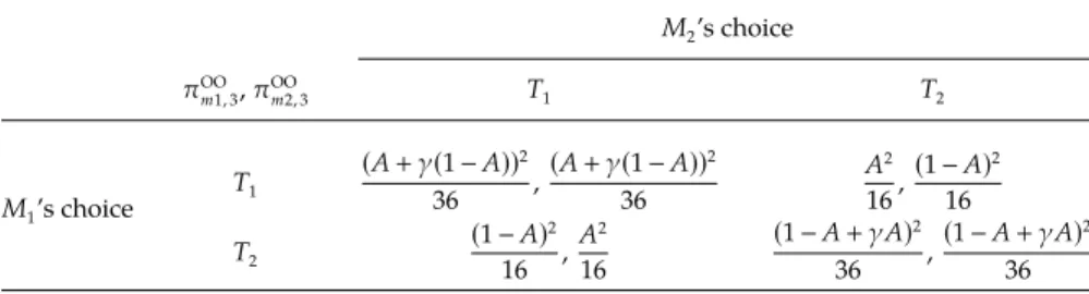
Table 1. Payoff Matrix for the Manufacturers’ Technology Choices in Scenario OO
M2’s choice
πOO
m1,3,πOOm2,3 T1 T2
M1’s choice
T1
(A+γ(1−A))2
36 ,
(A+γ(1−A))2
36
A2
16,
(1−A)2
16
T2
(1−A)2
16 ,
A2
16
(1−A+γA)2
36 ,
(1−A+γA)2
36
Case 3: Supplier invests in both technologies. In this case, both manufacturers can freely adopt any technol-ogy. The manufacturers’ technology choice equilibria in stage 3 are shown in Table 1, which presents the manufacturers’ profits given their technology choices.
The next proposition characterizes the equilibrium of stage 3’s manufacturer technology-choice game. Technically, multiple equilibria may arise, but we select one equilibrium following intuitive rules, which we will note after the proposition.
Proposition 3 (Equilibria with Two Open Technologies). When both manufacturers open their technologies and the supplier invests in both technologies, consider the stage 3 manufacturer technology choice game:
(i) ifγ≤1/2, the Nash equilibrium is
(T
1,T1) ifA≥ (3−2γ)/(5−2γ),
(T
1,T2) if 2/(5−2γ)<A<(3−2γ)/(5−2γ), (T
2,T2) ifA≤2/(5−2γ);
(ii) ifγ >1/2, the Nash equilibrium is
(T
1,T1) ifA≥1/2,
(T
2,T2) ifA<1/2.
Remark on Proposition 3(Equilibrium Refinement ).Tech-nically, multiple Nash equilibria arise in both subcases. In subcase (i), when (T
1,T2) is an equilibrium, so is (T
2,T1), in which M1 and M2 swap technologies and
payoffs. Two manufacturers adopting each other’s technology despite having their own is clearly not a realistic scenario; thus, we rule out this equilibrium. In subcase (ii), (T
1,T1) and (T2,T2) may both be
equilibria; however, one always Pareto dominates the other. After the dominated equilibrium is ruled out, Proposition3(ii) ensues.
the more favorable technology. Note that this risk pool-ing benefit is not fully available if one technology is closed or if the supplier does not invest in both tech-nologies. Therefore, it might drive manufacturers to open their technology as well as induce the supplier to invest in both technologies—even if eventually only one technology will be adopted. On the other hand, withAin an intermediate range (i.e., neither technol-ogy dominates the other) and a low spillover factor, the manufacturers introduce their technologies in their own markets to avoid competition.
Using the equilibria in stage 3, we can then calculate the firms’ expected profits in stage 2:
(i) ifγ≤1/2,
πOO
s,2
∫ 2/(5−2γ)
0
(1−A+γA)2
6 dA
+
∫ (3−2γ)/(5−2γ)
2/(5−2γ)
A2+(1−A)2
8 dA
+
∫ 1
(3−2γ)/(5−2γ)
(A+γ(1−A))2
6 dA−2K
1
12+
37+40γ−20γ2
18(5−2γ)3 −2K,
πOO
m1,2π OO
m2,2
∫ 2/(5−2γ)
0
(1−A+γA)2
36 dA
+
∫ (3−2γ)/(5−2γ)
2/(5−2γ)
A2
16dA
+
∫ 1
(3−2γ)/(5−2γ)
(A+γ(1−A))2
36 dA
1
48+
38γ−17
216(5−2γ)2;
(ii) ifγ >1/2,
πOO
s,2
∫ 1/2
0
(1−A+γA)2
6 dA
+
∫ 1
1/2
(A+γ(1−A))2
6 dA−2K
7+4γ+γ2
72 −2K,
πOO
m1,2π OO
m2,2
∫ 1/2
0
(1−A+γA)2
36 dA
+
∫ 1
1/2
(A+γ(1−A))2
36 dA
7+4γ+γ2
432 .
With all three cases analyzed, we can determine the supplier’s optimal decision on technology investment in stage 2. Define three thresholds for this purpose on the supplier’s investment cost:
βOO
1 (γ) ≡
1+γ+γ2
18 ,
βOO
2 (γ) ≡
74+80γ−40γ2− (5−2γ)3(−1+2γ+2γ2)
36(5−2γ)3 ,
βOO
3 (γ) ≡
1−γ2
24 .
Note that βOO
1 (γ) ≥max{βOO2 (γ), βOO3 (γ)}, βOO2 (γ)>0,
and βOO
3 (γ) ≥ 0 for all γ ∈ [0,1]. It is interesting to
observe that unlike Scenario OC, the supplier’s rev-enue is always larger when investing in two technolo-gies than in just one. For simplicity of notation, we further define
ˆ
β(γ) ≡
( βOO
2 (γ) ifγ≤1/2,
βOO
3 (γ) ifγ >1/2,
which is continuous at 1/2 and decreasing in γ. The following proposition characterizes the optimal and equilibrium outcomes in Scenario OO.
Proposition 4 (Scenario OO). When both manufacturers open their technologies,
(i) ifK≥βOO
1 (γ), the supplier invests in neither technol-ogy, andπOO
s,2πOOm1,2πOOm2,20;
(ii) ifβˆ(γ) ≤K< βOO
1 (γ), the supplier invests in only one technology, andπOO
s,2(1+γ+γ
2)/18−K,πOO
m1,2π OO
m2,2 (1+γ+γ2)/108;
(iii) ifK<βˆ(γ), the supplier invests in both technologies. Whenγ≤1/2,
πOO
s,2
1 12+
37+40γ−20γ2
18(5−2γ)3 −2K,
πOO
m1,2π OO
m2,2
1 48+
38γ−17
216(5−2γ)2;
otherwise,
πOO
s,2
7+4γ+γ2
72 −2K,
πOO
m1,2π OO
m2,2
7+4γ+γ2
432 .
Figure 3.Equilibrium Manufacturer Technology Strategies and Optimal Supplier Technology Investment
0 17/38 1
0.036 1/24 0.0442 1/18
1. {XX, Neither}
3. {OO, One}
8. {CC, Both} 4. {CC, Both}
5. {OO, One} 6. {CC, Both}
7. {OO, Both}
OC
K
1 ()
OC
2OC()
()
2. {OO, Both}
Notes. γ˜ is the solution in[0,1] to the equation ˆβ(γ)1/24, ˆγ (
√
6−1)/2≈0.725, andγOCis the solution in[0,1]to the equation
βOC 2 (γ)0.
technology. (In anticipation of this behavior, manu-facturers may in turn force the supplier to invest in both technologies by not opening their technologies; see Region 4 in Figure3.)
4.2. Stage 1: Manufacturer Technology Strategy
With the stage 2–4 subgames analyzed, we can finally characterize the stage 1 manufacturer technology strat-egy equilibrium and the ensuing stage 2 optimal technology investment decisions by the supplier. (See Figure3for an illustration of the outcomes; “OO” or “CC” means that both manufacturers open or close their technologies in equilibrium; “Neither,” “One,” or “Both” means that the supplier invests in neither, one, or both technologies as an optimal best response.)
In the stage 1 equilibrium analysis, we adopt the
trembling-hand refinement. A Nash equilibrium survives the trembling-hand refinement if the equilibrium is sustained even when each player has a small prob-ability of playing the off-equilibrium strategy. Such trembling captures possible errors in strategy execu-tions and/or the risk of a player behaving nonra-tionally. This is a widely accepted refinement that ensures the equilibria to be robust in practice where not all players are necessarily fully rational and perfectly execute their strategies. In our model, a unique equilib-rium survives this refinement. For convenience, we use “the unique perfect equilibrium” to represent either the unique subgame-perfect Nash equilibrium or the unique trembling-hand-perfect equilibrium. Moreover, for symmetry, when the supplier invests in one tech-nology, she is indifferent between the two technologies; thus, we do not specify exactly which technology she invests in.
4.2.1. High Investment Cost
Theorem 1 (High Investment Cost: Open Technology Can Incentivize Investment).SupposeK≥1/24.
(i) IfK≥βOC
1 (γ), the supplier invests in neither technol-ogy, regardless of the manufacturers’ technology strategies.
(ii) If1/24≤K< βOC
1 (γ), the unique perfect equilibrium of the stage 1 game is that both manufacturers open their tech-nologies. The ensuing outcome in stage 2 is as follows:
(ii-1) if max{1/24,βˆ(γ)} ≤ K< βOC
1 (γ) (or equiva-lently, γis large enough), the supplier invests in only one technology;
(ii-2) if1/24≤K<max{1/24,βˆ(γ)}(or equivalently, γis small enough), the supplier invests in both technologies.
Theorem 1 characterizes the equilibrium behavior when investing in a technology costs more than the supplier’s expected profit from doing so, i.e.,K≥1/24.
In case (i), where the technology investment cost is very high, the supplier never invests in any technology. This is a trivial case where all strategies are technically Nash equilibria, but these trivial equilibria have little practi-cal value. In this case, technologies are not cost-efficient enough for commercial adoption. In Case (ii), because
K≥1/24, the supplier would not invest in any
tech-nology if it were closed (see Proposition 1(i)). There-fore, both manufacturers open their technologies to incentivize supplier investment. Then, in subcase (ii-1), where spillover is relatively strong, the supplier invests in only one technology, because even when this tech-nology turns out to be less popular, the supplier is still guaranteed a sizable market because of the strong spillover from the absent market. Thus, the supplier indirectly benefits from technology risk pooling and saves the high investment cost for one technology. In subcase (ii-2), where spillover is relatively weak, it is too risky to bet on a single technology, and thus the supplier invests in both technologies to take full advan-tage of the technology risk pooling (see the discussion following Proposition3), which benefits the manufac-turers as well.
When technology investment costs are too high for the supplier to invest in competing closed technolo-gies, open technology can induce supplier investment. This insight from Theorem 1 confirms our intuition in the introduction. The case of Tesla’s and Toyota’s open technology “arms race” likely falls into this cate-gory. The automotive industry is highly capital inten-sive, and to boost industry confidence, both Tesla and Toyota chose to open their technologies. This might have been partially encouraged by Tesla’s open-technology strategy.
4.2.2. Low Investment Cost
The unique equilibrium of the stage 1 game is that both manufacturers close their technologies. The ensuing stage 2 outcome is that the supplier invests in both technologies.
When investing in a technology costs less than the supplier’s expected profit from doing so, and spillover is relatively weak, the equilibrium outcome is always that both manufacturers close their technologies and the supplier invests in both technologies. However, this equilibrium actually emerges for three differ-ent reasons, which result in differdiffer-ent off-equilibrium outcomes.
First, when K< βOC
2 (γ) (i.e., the investment cost is
very low), the supplier will invest in both technologies regardless of whether they are open or closed. Hence, the manufacturers do not need to incentivize supplier investments. The relatively weak spillover means that the potential market size for a popular technology (including the spillover from the other technology) is small. As a result, no manufacturer wants to unilat-erally open his technology for fear of a small future market. Therefore, both manufacturers close their tech-nologies in a Nash equilibrium.
Second, whenβOC
2 (γ) ≤K<βˆ(γ)(i.e., the investment
cost is in an intermediate range within[0,1/24]), the
supplier will not invest in a technology if it is the only closed technology. In other words, if one technology is open and the other is closed, the supplier will invest only in the open technology. Again, the relatively weak spillover results in both manufacturers closing their technologies. As a result, the supplier has to invest in both technologies.
Third, when ˆβ(γ) ≤ K<1/24 (i.e., the investment
cost is relatively high within [0,1/24]), the supplier
will invest in only one open technology if at least one technology is open, and otherwise will invest in both technologies if spillover is not overly strong, i.e.,
γ <γˆ (where ˆγ > 17/38). Thus, both manufacturers
close their technologies to avoid being forced to com-pete in a market that is potentially small due to weak spillover; as a result, the supplier invests in both tech-nologies. Since we have shown that open technologies can encourage supplier investment, the fact thatclosed
technologies can also pressure the supplier to invest in more technologies (from one to two) is perhaps sur-prising and counterintuitive.
Theorem 3 (Low Investment Cost and Strong Spillover: Open Technology Can Generate Risk-Pooling Benefit). ConsiderK<1/24andγ≥17/38.
(i) When K < βOC
2 (γ), the unique equilibrium of the stage 1 game is that both manufacturers close their technolo-gies. In stage 2, the supplier invests in both technolotechnolo-gies.
(ii) When βOC
2 (γ) ≤K<βˆ(γ), the unique perfect equi-librium of the stage 1 game is that both manufacturers open their technologies. In stage 2, the supplier invests in both technologies.
(iii) WhenK≥βˆ(γ), letγˆ( √
6−1)/2≈0.725:
(iii-1) If γ <γˆ, the unique equilibrium of the stage 1 game is that both manufacturers close their technologies. In stage 2, the supplier invests in both technologies.
(iii-2) If γ≥γˆ, the unique perfect equilibrium of the stage 1 game is that both manufacturers open their technolo-gies. In stage 2, the supplier invests in one technology.
In case (i) of Theorem3, the equilibrium outcome is the same as in the first scenario discussed after The-orem 2. In this case, the manufacturers do not need to incentivize the supplier’s technology investment, and the not-overly-strong spillover leads both manu-facturers to close their technologies in a Nash equilib-rium. However, unlike the case in Theorem 2 where the spillover is even weaker, in this case, if both manu-facturers were to open their technologies, the supplier would invest in both technologies, and the manufac-turers would be better off because of technology risk pooling. This is a classic prisoner’s dilemma situation.2 To reiterate, with low technology investment costs and an intermediate level of spillover, manufacturers may be faced with the prisoner’s dilemma and choose to close their technologies despite the full risk-pooling benefit enabled by two open technologies. It means that in such scenarios where firms will not unilateral open their technologies, there may be potential for col-laborative technology sharing, such as cross licensing (i.e., an agreement between two parties to grant each other rights to their respective patents). In practice, cross licensing is fairly common; however, it usually serves as a means for firms to trade patents as well as to avoid or settle patent infringement disputes. In such applications, the patents being cross-licensed are often for unrelated technologies. Our result suggests that two firms may use cross licensing to allow each other access to competing technologies that serve fun-damentally similar functions to enjoy technology risk pooling and avoid the prisoner’s dilemma.
In case (ii) of Theorem3, as in the second scenario discussed after Theorem2, the supplier will not invest in a technology if it is the only closed technology. How-ever, unlike that scenario with weak spillover, when spillover is not overly weak, all parties benefit from risk pooling when both manufacturers open their tech-nologies. Since spillover is not very strong, the sup-plier has to invest in both technologies to benefit from full risk pooling. As a result, both manufacturers open their technologies, and the supplier invests in both technologies.
In case (iii) of Theorem 3, the supplier’s incentive resembles the third scenario discussed after Theo-rem 2; namely, the supplier will invest in only one open technology if at least one technology is open. In subcase (iii-1), if spillover is not overly strong, i.e.,
competition, and thus both manufacturers close their technologies. By contrast, in subcase (iii-2), the rela-tively strong spillover means that even a single open technology is guaranteed a sizable market and makes significant risk pooling possible. Therefore, both man-ufacturers open their technologies to benefit from risk pooling, and the supplier invests in only one technol-ogy to balance risk pooling and investment cost.
It can be seen that with an intermediate level of spillover, i.e., 17/38≤γ <γˆ, somewhat surprisingly,
the equilibrium manufacturer technology strategy is nonmonotonic in the technology investment cost. More specifically, as the investment cost increases, the equi-librium behavior changes from {CC, Both} to {OO, Both}, and then back to {CC, Both}. The explanation is as follows. First, when the investment cost is low enough, the supplier will always invest in both tech-nologies whether the manufacturers open or close their technologies. Although {OO, Both} generates higher profits than {CC, Both}, manufacturers have an incen-tive to unilaterally close their technologies to deter competition. That is the prisoner’s dilemma. Second, as the investment cost increases, the supplier will not invest in a technology if it is the only closed technology. As a result, both manufacturers open their technolo-gies when spillover is not overly weak, and the supplier invests in both technologies. Third, as the investment cost rises further, the supplier will invest in only one open technology if at least one technology is open; oth-erwise, she will invest in both technologies if spillover is not overly strong. As mentioned, both manufacturers prefer closed technologies. The second scenario occurs when spillover is not overly weak, and the third sce-nario occurs when spillover is not overly strong. As a result, this nonmonotonic behavior is observed only with an intermediate level of spillover. The nonmono-tonic equilibrium technology strategies also lead to all
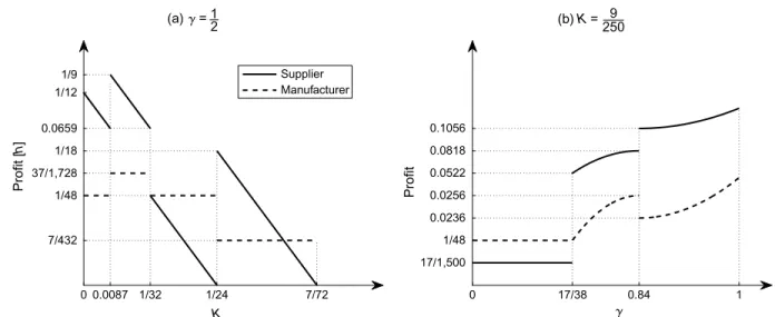
Figure 4.Firms’ Expected Profits
0 0.0087 1/32 1/24 7/72
7/432 1/48 37/1,728 1/18 0.0659 1/12 1/9
K
Profit [
h
]
Supplier Manufacturer
0 17/38 0.84 1
17/1,500 1/48 0.0236 0.0256 0.0522 0.0818 0.1056
Profit
(b)K= 9 250 (a) =
2 1
players’ profits being nonmonotonic in the technology investment cost (see Figure4(a)).
Another interesting observation is that manufactur-ers’ expected profits are nonmonotonic in the spillover factor (see Figure 4(b)). On the one hand, when
γ∈ [0,0.84], the manufacturers’ expected profits are
increasing inγ. The reason is that for low technology investment costs, when spillover becomes stronger, the manufacturers tend to shift from closing to opening their technologies to benefit from risk pooling. On the other hand, whenγcontinues to increase, the supplier invests in fewer technologies—because one open tech-nology already provides significant risk pooling for the supplier—and that causes the manufacturers’ profits to drop. However, it can be observed that the supplier’s profit is always increasing inγ.
Theorem 3 demonstrates that the spillover effect greatly influences competing firms’ technology strate-gies, particularly with low technology investment costs. In general, stronger spillover tends to encour-age open technologies for two reasons: first, stronger spillover better mitigates the detrimental effect of com-petition resulting from opening technologies; second, stronger spillover improves technology risk-pooling benefits.
4.2.3. Summary. Our analyses confirm the intui-tion that open technologies can encourage supplier investments. In addition, we present below a list of somewhat unexpected managerial insights. The num-bered equilibrium cases in the summary are defined in Figure3.
• Besides encouraging supplier investments, open technologies yield another benefit, namely, technol-ogy risk pooling. This benefit is realized with either high investment costs (as in equilibrium cases 2 and 3) or strong spillover (as in equilibrium cases 5 and 7), resulting in both manufacturers opening their tech-nologies.
• With high technology investment costs or strong spillover, as the investment cost rises, the manufactur-ers tend to open their technologies to induce supplier investments. However, as they do so, the supplier may invest in fewer technologies due to the higher invest-ment cost (see the change from equilibrium case 6 to 2 to 3 and from equilibrium case 8 to 7 to 5 whenγ≥γˆ).
• With low technology investment costs and inter-mediate spillover, manufacturers may be faced with the prisoner’s dilemma and close their technologies despite the benefits of technology risk pooling if both technologies are open (see equilibrium case 8, 17/38< γ <γˆ). In this case, there is potential for collaborative technology sharing, such as cross licensing.
• As the investment cost increases, manufacturers may become less willing to open their technologies (from equilibrium case 7 to case 4), and their equilib-rium profits mayincrease(from equilibrium case 8 to case 7; see the first two segments of Figure4(a)).
5. Extensions
Owing to the complexity of the problem, we utilize a simplified base model to flush out the fundamental insights. It is necessary to check whether these insights are robust when certain assumptions are relaxed or modified. In this section, we investigate three main extensions of the basic model: (1) sequential order quantity decisions; (2) asymmetric technologies; (3) al-ternative source of supply. While these extensions are mostly tractable, it is difficult to present full results because of their complexity. Therefore, we will present the most representative results.
5.1. Sequential Order Quantity Decisions
In Section3, we discussed whyM1andM2
simultane-ously determining order quantities after choosing their technologies is a more appropriate assumption for our motivating example (see Remarks on the Base Model). Nevertheless, sequential order quantity decisions may fit certain business cases better; hence, we investigate such a model. The comparison between sequential and simultaneous quantity competitions is well studied, and a key insight is that in sequential competition, the first mover has an advantage over the second mover (see Fellner1949).
Specifically, we modify our base model so that when
M1 and M2 adopt the same technology, the original
technology owner determines his order quantity before
the other manufacturer in stage 4. Such a model cap-tures business cases in which product development cycles are short and original technology owners have significant first-mover advantages. The detailed anal-ysis can be found in Supplement A in the online appendix; we illustrate only the stages 1 and 2 equilib-rium outcomes in Figure5.
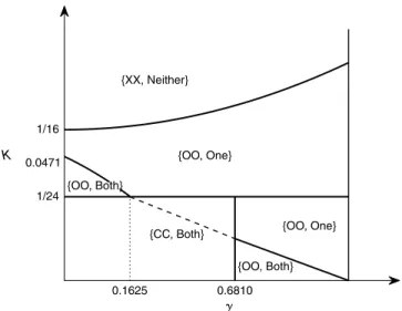
The foremost observation is that the equilibrium structure is largely consistent with the base model (see Figure3). This shows that most of our main insights are robust under sequential order quantity decisions. There are a few other notable observations, which we discuss below. They are mostly driven by the fact that when both manufacturers adopt the same technology, sequential order quantity decisions increase the profits of the supplier and the technology owner, but reduce the other manufacturer’s profit, due to an increased order quantity from the technology owner.
First, the region with the equilibrium {OO, One} expands against the {XX, Neither} region. Under sequential order quantity decisions, the supplier earns more from an open technology; hence, there is a stronger incentive for the supplier to invest in an open technology.
Second, one may expect that there is more incen-tive for a manufacturer to open his technology, because when the competitor adopts his technology, the first-mover advantage improves his profit. However, sur-prisingly, the first-mover advantage may actually cause a manufacturer to close his technology when the investment cost and spillover are in an intermediate range. In such cases, the equilibrium is {CC, Both} under sequential order quantity decisions, in contrast with {OO, Both} under simultaneous order quantity decisions (equilibrium case 7 in Figure 3). The rea-son is that under sequential order quantity decisions,
Figure 5. Equilibrium Outcomes Under Sequential Order Quantity Decisions
{XX, Neither}
{OO, One}
{CC, Both}
{OO, Both}
0.1625 0.6810
1/24 0.0471 1/16
K
when both manufacturers adopt the same technology, the supplier’s profit is also improved. As a result, in those cases, the supplier only invests in one technol-ogy when both technologies are open. In anticipation, both manufacturers close their technologies and force the supplier to invest in both technologies.
5.2. Asymmetric Investment Costs
In this section we investigate technologies that are asymmetric in investment cost. We denote the invest-ment costs of technologies 1 and 2, respectively, byK1
and K2, and assume without loss of generality that K1≤K2. The detailed analysis can be found in
Sup-plement B in the online appendix; we illustrate only the stage 1 and 2 equilibrium outcomes with vary-ingK1andK2forγ1/2 in Figure6, where “X”
indi-cates that either an open or a closed technology of the corresponding manufacturer can constitute an equilib-rium, andTi denotes the technology that the supplier invests in. In addition, Figure S1 in Supplement B in the online appendix, illustrates equilibrium outcomes with other γvalues, which have similar structures as Figure6.
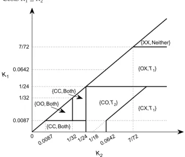
We list some notable observations about Figure 6. First, on the lineK1K2, the equilibria replicate those
in Figure3forγ1/2. In the immediate neighborhood
ofK1K2, the equilibria remain the same except near a
single point (K11/24), where an asymmetric
equilib-rium arises. Therefore, the equilibria characterized for the symmetric base model are mostly robust under not-too-significant technology investment cost asymmetry. Second, with asymmetric investment costs, asym-metric equilibria may arise, and in most cases manufac-turer 2 opens his technology. (In those scenarios with
Figure 6.Equilibrium Outcomes Under Asymmetric Fixed CostsK1≤K2
{CC, Both} {OO, Both}
{CC, Both}
{XX, Neither}
{CO,T2}
{OX,T1}
{CX,T1}
0.0087 1/32 1/2 4
1/180.0642 7/72
0.0087
0 1/32 1/24 0.0642 7/72
K2 K1
an asymmetric equilibrium, if there is only one equi-librium, it must be manufacturer 2 who opens his tech-nology, and if there are multiple equilibria, there must exist an equilibrium in which manufacturer 2 opens his technology.) Recall that K1≤K2; in other words, T2 is the disadvantaged technology that requires a
higher investment cost. The fact that the disadvan-taged technology is more often open is intuitive: since the supplier is otherwise likely to invest in the advan-taged technology, the manufacturer’s only hope is to influence the supplier by opening his technology. This strategy is evident in the equilibrium {CO,T2}, where
the supplier invests in the more expensive but open technology 2. However, when the investment costs are highly asymmetric with T2 being much more
expen-sive, this strategy no longer works, as is evident in the equilibrium {CX,T1}, where the supplier always invests in the less costly T1 regardless of whether
manufac-turer 2 opens or closes his technology.
Third, interestingly enough, in one equilibrium sce-nario, {OX,T1}, it is the advantaged manufacturer M1
who opens his technology. Note that this occurs with relatively high investment costs for both technologies. In this case, even the advantaged manufacturer needs to incentivize supplier investments, and the disad-vantaged manufacturer’s technology strategy becomes irrelevant.
5.3. Asymmetric Market Preferences
In this section we investigate technologies that are asymmetric in market preference. We adopt a Bernoulli market preference distribution as opposed to the uni-form distribution in the base model, which helps us manage the model complexity but also serves as a robustness check on the market preference distribution (we confirm that the base model’s equilibrium struc-ture remains qualitatively unchanged under the new distribution in the case of symmetric market prefer-ences). To be specific, we assume that the market share that prefers technology 1,A, follows a Bernoulli distri-bution that takes value 1 with probabilityαand 0 with probability 1−α, and that the market share that prefers
technology 2 is 1−A. In other words, the entire market
either prefersT1 or prefersT2. Without loss of
gener-ality, we assumeα≥1/2. This means thatT
1’s market
share is stochastically larger thanT2’s; thus, M1 is the
advantaged manufacturer. The detailed analysis can be found in Supplement C in the online appendix; we illustrate only the stage 1 and 2 equilibrium outcomes with varyingαandKforγ1/2 in Figure7. The
nota-tion is the same as in Figure6. In addition, Figure S2 in Supplement C in the online appendix illustrates equi-librium outcomes with otherγvalues, which have sim-ilar structures as Figure7.