Do Phonologically Active Classes Cause Warping of the Perceptual Space?
Emily Moeng
A thesis submitted to the faculty of the University of North Carolina at Chapel Hill in partial fulfillment of the requirements for the degree of Master of Arts in the Department of Linguistics.
Chapel Hill 2012
ii © 2012
iii ABSTRACT
EMILY MOENG: Do phonologically active classes cause warping of the perceptual space? (Under the direction of Elliott Moreton)
Perceptual warping has been observed in various domains, both linguistic and
iv
ACKNOWLEDGEMENTS
I would like to thank the members of my committee, Elliott Moreton, Jen Smith, and Katya Pertsova, for their guidance and detailed comments, as well as Chris Wiesen at the Odum Institute for his statistical advice. I would also like to thank my officemate Kline Gilbert for greatly increasing the enjoyability of my grad school experience.
Finally, I would like to thank Chris O’Neill. I greatly appreciate not only the large
v
TABLE OF CONTENTS
LIST OF TABLES ... viii
LIST OF FIGURES ... ix
CHAPTER 1. Introduction ... 1
1.1.Importance of answering whether phonologically active classes warp the perceptual system ... 2
CHAPTER 2. Conceptual Background ... 5
2.1. Turkish front/back vowel harmony ... 6
2.2. Terbeek: Possible perceptual warping due to phonologically active classes ... 7
2.3. Artificial-language studies ... 11
2.3.1. Importance for present study ... 15
2.4. Perceptual warping caused by categories ... 15
2.4.1. Relevant and irrelevant dimensions... 22
2.4.2. Summary of perceptual warping ... 24
2.4.3. Importance for present study ... 25
2.5. Category Ratios ... 26
2.5.1. Justification for Category Ratios ... 26
2.5.2. Calculation of Category Ratios ... 29
CHAPTER 3. Methods ... 40
3.1. Participants ... 40
3.2. Stimuli ... 40
vi Pre-training Similarity
Training
Post-training Similarity
Evaluation
Questionnaire
CHAPTER 4. Predictions ... 47
CHAPTER 5. Data analysis ... 50
CHAPTER 6. Results ... 55
6.1. Did participants “learn” front/back vowel harmony? ... 55
6.2. Is there perceptual warping associated with learning a language with front/back vowel harmony? ... 56
6.2.1. Distances ... 57
Backness Control Backness group in reference to the Control group Analysis of variance 6.2.2. Category Ratios ... 63
Backness Control Backness group in reference to the Control group Analysis of variance CHAPTER 7. Discussion... 70
7.1. Summary of results ... 70
7.2. What numerical results suggest ... 71
7.2.1. Any training causes changes in similarity judgments ... 71
vii
7.4. Do phonologically active classes warp the perceptual space? ... 76
CHAPTER 8. Conclusion ... 77
8.1. Reasons for further study ... 77
8.2. Present experiment design ... 79
8.3. Improvements on experiment design... 80
8.3.1. Participants require more training ... 80
8.3.2. More accurate similarity judgments with more vowels... 80
8.3.3. Confusion task in place of a similarity task ... 81
8.4. Concluding remarks ... 82
viii
LIST OF TABLES
Table
ix
LIST OF FIGURES
Figure
1. 2-dimensional depiction of similarity judgments of vowels of English,
German, Thai, and Turkish ... 9
2. Hypothetical effects of categorizing objects (chickens) on perception ... 16
3. Hypothetical effect of categorizing objects (light vs. dark) on perception... 17
4. Stimuli used in Goldstone (1994b) experiment ... 23
5. Three hypothetical effects of categorization ... 27
6. Stimuli used in Goldstone (1994b) experiment ... 28
7. Results of Goldstone (1994b) experiment ... 29
8. Example of the calculation of a Within-category ratio xy ... 30
9. Example of the calculation of an Across-category ratio xy ... 32
10. Category Ratios calculated from stimuli consisting of drawings of microorganisms (Livingston et al., 1998)... 34
11. Category Ratios calculated from stimuli consisting of photographs of chick genitalia (Livingston et al., 1998) ... 34
12. Category Ratios calculated from stimuli consisting of squares varying in brightness and in size (participants trained on size) (Goldstone, 1994b) ... 35
13. Category Ratios calculated from stimuli consisting of squares varying in brightness and in size (participants trained on brightness) (Goldstone, 1994b) ... 35
14. Category Ratios calculated from stimuli consisting of tense and lax vowels (Kondaurova and Francis, 2010) ... 36
15. Category Ratios calculated from stimuli consisting of Korean stop contrasts (Within-category Ratios) (Francis and Nusbaum, 2002) ... 37
16. Category Ratios calculated from stimuli consisting of Korean stop contrasts (Across-category Ratios) (Francis and Nusbaum, 2002) ... 37
17. Category Ratios calculated from stimuli consisting of vowels (Within- category Ratios) (Terbeek, 1977) ... 38
x
19. Image from instructions given to participants ... 42
20. Image from instructions given to participants ... 42
21. Simplified model of experiment on which predictions are made. ... 47
22. Hypothetical triangles illustrating that some scaling is necessary... 50
23. Scaling constants. ... 52
24. Box plot of the number missed in the Evaluation portion ... 55
25. Distances of Backness group ... 58
26. Distances of Control group ... 59
27. Distances of Backness group minus distances of Control group ... 60
28. Category Ratios of the Backness group... 64
29. Category Ratios of the Control group ... 65
30. Category Ratios of Backnes group and Control group ... 66
31. Category Ratios of Backness group minus Category Ratios of Control group ... 67
1
CHAPTER 1
INTRODUCTION
Cognitive processes do not deal directly with raw sensory data. Whether visual or auditory, sensory data is first filtered through an organism's perceptual system in order to facilitate the processing of the “blooming, buzzing confusion” (James, 1890). However the perceptual system is not a static system, with a one-way flow of information from sensory data to perception to higher-level cognition. Instead, the perceptual system is subject to mutations dependent on the needs of the organism. These needs of the organism come from, among other things, categories1 that the organism has formed (Goldstone and Hendrickson, 2010). Therefore higher-level cognition, such as categories, influences the perceptual system. This two-way flow of information and malleability of the perceptual system facilitates learning within an organism. Perception is warped so as to aid categorization, which results in greater efficiency (Goldstone et al., in press). That is, the perceptual space can be distorted compared to the physical (acoustic or visual) space.
While many studies have found that the existence of categories will warp the perceptual system, one study conducted by Dale Terbeek (1977) suggests, but does not conclude, that the existence of phonologically active classes2 shows similar perceptual warping effects. That is, it may be the case that the concept of a [+back] category and a [-back] category in speakers of languages with front/back vowel harmony warps the perceptual system. However, Terbeek was
1
A category is defined as a classificatory division.
2
unable to draw firm conclusions from his study about the possible role of phonologically active classes on the perceptual space.
The central goal of this thesis is to replicate Terbeek’s experiment correcting one issue which was noted by Terbeek in his study. This is done by training participants on an artificial language with front/back vowel harmony. Participants are trained on an artificial language which groups front vowels into one category and back vowels into another category (in the form of front/back vowel harmony), and are asked to make similarity judgments of the vowels used in the language before and after training. Similarity judgments are used to infer participant perceptual spaces to determine whether the perceptual space has been warped after learning an artificial language with front/back vowel harmony.
Results do not reach statistical significance, but further study is recommended as numerical results suggest that phonologically active classes do warp the perceptual system. Significance of answering more firmly whether or not phonologically active classes warp the perceptual space is discussed. It is argued that the main question “Do phonologically active classes warp the perceptual system?” is an important question to pursue because its answer has the potential of shedding light on further questions of interest in linguistics.
1.1. Importance of answering whether phonologically active classes warp the perceptual
system
Why is it important to answer whether phonologically active classes warp the perceptual system? The answer to this question can help shed light on larger issues within linguistics, in particular which aspects of language are special to language, and what the relationship is between artificial and natural language.
3
that some attributes of language are special to language while others are shared by other, non-linguistic aspects of cognition (Jackendoff and Pinker, 2005). If this is the case, the connection between general cognitive properties and linguistic properties needs to be tested on a property-by-property basis. This paper addresses whether one of these properties, the existence of
phonologically active classes of sounds, can be reduced to terms of a property which has been observed in general cognition.
i. How much of language is due to general cognition? Specifically, do phonologically active sounds behave in a way that is special to language?
This paper also addresses how useful artificial languages can be in informing us about first language acquisition. While there are many studies which involve training participants on some artificial language, it is unknown if we can we safely draw conclusions about L1 acquisition from the behavior of participants trained on an artificial languages (for a discussion, see Moreton and Pater, 2012). Artificial languages are different from natural languages in that there is already a language in place for the artificial-language learner (ie. their native language). In this way, language learning may be more analogous to L2 acquisition. On top of which, artificial-language experiments which are done on adults have to deal with the added complication that any proposed critical period for language learning has already passed. As was the case with the question of how special language is in comparison to other cognitive domains, this is likely another issue which must be tested property-by-property.
4
5
CHAPTER 2
CONCEPTUAL BACKGROUND
This thesis is concerned with the possible connection between phonologically active classes of sounds and warping of the perceptual space. As defined by Jeff Mielke (2008), a phonologically active class is a group of sounds which, to the exclusion of all other sounds in the language's inventory, either participate in or trigger a phonological rule, or exemplify a static distributional restriction. The perceptual space is defined as the psychological stimulus space.
Although warping of the perceptual space has been demonstrated for individual speech sounds, both for consonants (“categorical perception”, see the Note on terms #1 in Section 2.3) and for vowels (the Perceptual Magnet Effect), only one experiment known to the author has been conducted which hints at a possible warping of the perceptual space due to the existence of a phonologically active class. This experiment, conducted by Dale Terbeek, finds that Turkish speakers judge back vowels to be more similar to one another and front vowels to be more similar to one another, when compared to speakers of English, German, Swedish, or Thai. If a perceptual space is inferred from the similarity judgments given in this experiment, the Turkish perceptual space is compressed along the height dimension, in comparison to the perceptual spaces of other speakers. Terbeek (1977) suggests that this difference in the perceptual space of Turkish speakers is caused in part by Turkish having front/back vowel harmony. This thesis attempts to revise a weakness which Terbeek noted in his experiment design, by replicating Terbeek’s experiment using artificial-language training.
6
of artificial-language training in place of natural language, the use of artificial-language training is briefly reviewed (Section 2.3). Following this, perceptual warping is reviewed, and parallels are drawn between perceptual warping of speech sounds and perceptual warping of non-linguistic stimuli (Section 2.4). Finally, a new measure called a Category Ratio is introduced to determine whether perceptual warping has occurred (Section 2.5).
2.1. Turkish front/back vowel harmony
Within Turkish, all vowels (and consonants [l] and [k]) within a word agree in their specification for backness (Clements and Sezer, 1982). Affixes alternate so as to agree in backness with the nearest root vowel. Roots do not alternate. Apparent exceptions can be explained by the presence of opaque segments in the underlying representation (Clements and Sezer, 1982).
nom.sg. gen.sg. nom.pl. gen.pl.
‘rope’ ip ip-in ip-l er ip-l er-in
‘end’ son son-un son-lar son-lar-ɨn
Table 1. Subset of table taken from Clements and Sezer (1982) showing front/back vowel harmony pattern within
Turkish. ‘l ’ is palatal, and ‘ɨ’ indicates high back unrounded vowel.
As can be seen in Table 1, the vowel in the affix will alternate so that it agrees in backness with the root. For example, the genitive singular affix is [in], which contains a front vowel, when it is attaching to the root [ip], which contains a front vowel. However, when attaching to the root [son], which contains a back vowel, the genitive affix is [un], which also contains a back vowel.
7
2.2. Terbeek: Possible perceptual warping due to phonologically active classes
Similarity judgments of speech sounds vary among speakers of different languages. This variation is caused by a range of factors. For example, Johnson (2003) demonstrates that
similarity judgments of vowels will be affected by whether or not a vowel belongs to a speaker’s linguistic inventory. In addition, and of most interest for the present study, a study done by Dale Terbeek (1977) suggests that similarity judgments may be affected by phonologically active classes.
In his study, Terbeek tested 7 speakers of 5 different languages: English, Turkish, Thai, Swedish, and German. His stimulus set consisted of 12 recorded monophthongs in the context [bəb__ ]. These monophthongs were [i y u e ø o æ ʌ ɑ ɨ ɚ ɑr ]. He presented participants with all possible triplets of these 12 sounds, giving each participant a total of 220 triads to listen to. Each participant was asked to judge which pair of each triad sounded the most similar, and which pair sounded the most dissimilar.
Terbeek analyzed the dissimilarity matrices using INDSCAL (INDividual Differences SCALing, also known as PARAFAC). For those familiar with classical multi-dimensional scaling, INDSCAL is similar to classical multi-dimensional scaling in that its purpose is to represent points in some N-dimensional space. In the case of Terbeek’s experiment, each of these points represents one of the 12 stimulus vowels, and the distance between any two points represents the judged similarity between those two vowels. Therefore, two points which are close to one another represent vowels which speakers judged to be similar to one another, and two points which are far apart represent vowels which speakers judged to be not very similar to one another. This
N-dimensional space can be thought to represent the speaker’s perceptual space.
8
Private spaces on the other hand are obtained by systematically distorting the Group space according to a Salience matrix. Each of these Private spaces represents only one dissimilarity matrix. The Salience matrix is a set of weights -- one for each dimension of the N-dimensional configuration. For example, suppose two dissimilarity matrices are analyzed using INDSCAL, each of which represents a different set of participants. If the dissimilarity matrix representing participants from Set A returns a Salience matrix with a high number corresponding to the weight placed on Dimension X while the dissimilarity matrix representing participants from Set B returns a Salience matrix with a low number corresponding to the weight placed on Dimension X, participants from Set A placed greater importance on Dimension X than participants from Set B for whatever task was given (see “INDividual Differences SCALing: INDSCAL,” n.d.).
Using INDSCAL, Terbeek obtained five Private spaces – one representing speakers from each of the five languages used (English, Turkish, Thai, Swedish, and German). The best-fit INDSCAL configuration consisted of 6 dimensions, one of which corresponded to the dimension of tongue backness. He found that Turkish speakers had a higher number in the Salience matrix which corresponded to the tongue backness dimension. In other words, Turkish speakers placed more importance on the tongue-backness dimension compared to the English, Thai, German, and Swedish speakers. Terbeek suggested this was due to Turkish having front/back vowel harmony as a phonological rule.
9
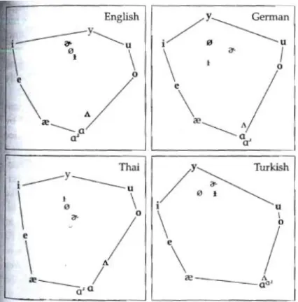
Figure 1. Figure obtained from Johnson (2003). 2-dimensional perceptual vowel spaces for listeners who speak English, German, Thai, and Turkish, computed from Terbeek’s dissimilarity matrices. Non-bold symbols represent sounds which are not part of the language’s inventory.
Terbeek’s findings (and Johnson’s 2-dimensional illustrations of those findings) are important because they show first, that perceptual spaces are in part dependent on the language spoken by the participant. While all participants heard the exact same acoustic signal (ie. the [bəbi] sound clip was the same sound clip for all participants), their similarity judgments of those acoustic signals were determined by which language they spoke. This illustrates a disjoint between the physical space (the acoustic signal), and the perceptual space (the psychological space), and is demonstrated in multiple other studies, which are discussed in Section 2.3.
10
emphasize the backness dimension because they have a phonological rule which highlights the affinity between all back vowels and the affinity between all front vowels. This in turn shows up as greater judged similarity of back vowels to other back vowels, and of front vowels to other front vowels, as compared to the similarity judgments made by non-Turkish speakers. This seems to be supported in that the Turkish speakers judged [u] and [o], two back vowels, to be the most similar as compared to the similarity judgments of the other non-Turkish speakers. They also judged [i] and [e], two front vowels, to be the most similar as compared to the similarity judgments of the other non-Turkish speakers.
11
Hypothesis 1 Terbeek’s findings are due only to poor matching of stimulus vowels to Turkish native vowels
Hypothesis 2 Terbeek’s findings are due in part to front/back vowel harmony in Turkish
Table 2. Possible explanations for Terbeek’s findings.
The possible reasons for Terbeek’s findings that Turkish speakers judge back vowels as being more similar to one another and front vowels as being more similar to one another are summed up in Table 2. Terbeek’s findings about similarity judgments made by Turkish speakers may be caused only by a poor fit of stimulus vowels to participant native vowels (Hypothesis 1). Or, Terbeek’s findings may reveal something more interesting: the differences in similarity
judgments in Turkish speakers may be, at least partially, caused by Turkish having a phonological rule of front/back vowel harmony. This is the only study known to the author which makes a connection between phonological rules and similarity judgments.
Why should Hypothesis 2 even be considered? That is, why would front/back vowel harmony explain the results found by Terbeek? It may be the case that what is being seen is no more than a simple case of perceptual warping caused by the existence of two categories: one consisting of front vowels, and another consisting of back vowels. This possibility will be reviewed in Section 2.4. But first, since this experiment will be replacing natural language with an artificial language, studies using artificial languages will be briefly reviewed.
2.3. Artificial-language studies
The present study trains participants on a mini language with front/back vowel harmony. Since this is an artificial-language study, it is worth noting the strengths and weaknesses of using artificial languages in experiments.
12
2008). Infants also show evidence of learning an artificial language with a phonological pattern relying on the knowledge of a phonologically active class defined as [-voice] speech segments (Saffran and Thiessen, 2003). Further, it does not seem to be the case that the infants in these studies simply memorize the individual segments which belong to these phonologically active classes, because it was more difficult for the infants to learn more formally complex
phonologically active classes, such as one consisting of both [+nasal] and [-continuant] segments. If infants simply memorized individual segments, a class consisting of segments which can be either [+nasal] or [-continuant] ( [+nasal] ˄ [-continuant] ) should be no more difficult to learn than a class consisting of just [+continuant] segments.
Adults have also been successful in learning artificial phonology. Most relevant for the present study, an adult participant trained on an artificial language with vowel harmony will do noticeably better than chance after just 15-20 minutes of training (Moreton, 2008; Pycha et al., 2003). In the present study, participants are trained for around 30 minutes, but only one (whose data was not used) reported noticing a pattern in the vowels when asked upon completion of the experiment. This shows that learning a vowel harmony pattern can be done quickly and implicitly, just from repeated exposure to “words” which conform to a vowel harmony pattern.
2.3.1. Importance for present study
13
a language with front/back vowel harmony with the perceptual space of English-speaking
participants trained on a language with no pattern in its vowels. The English-speaking participants who are trained on a language with front/back vowel harmony will represent the equivalent of the Turkish speakers in Terbeek’s study, and since English does not have a phonologically active class consisting of [+back] vowels or [-back] vowels (Mielke, 2008), the English speakers who are trained on a language with no pattern in its vowels will represent the equivalent of the non-Turkish speakers in Terbeek’s study, all of whom did not speak a language with front/back vowel harmony. All speech segments used within the artificial language will be designed to match native English vowels. Since all participants are native English speakers and all stimulus speech sounds will be prototypical English speech sounds, the main confounding factor within Terbeek’s study, which was that similarity judgments may have been affected by poor matching of stimulus vowels to native vowels, will be avoided.
As discussed in Moreton and Pater (2012), one potential point of criticism for these types of experiments is whether artificial languages can be used to draw conclusions about natural first language acquisition, especially when the participants are adults. This concern is justified, as many linguists assume a qualitative difference even between first and second language acquisition, due to the belief of a critical period in language acquisition, as well as the very different mental canvases onto which linguistic data is being placed (ie. no language exists for the L1 learner, but a language is already in place for an L2 learner and for an artificial-language learner).
14
combination of the two views -- that artificial-language learning shares some, but not all, mechanisms in common with first language acquisition. Because of this, different aspects of language need to be tested. A good indication that shared mechanisms are being employed is if results from artificial-language experiments mirror typological findings.
Therefore, in addition to attempting to strengthen Terbeek’s findings by replicating them in the lab, this study will also attempt to use this mirroring criteria to show that perceptual warping is something that natural-language acquisition and artificial-language learning share. In order for Terbeek’s results to be replicated in the lab, two things must be true. First, similarity judgments of Turkish speakers must have been affected by perceptual warping due to front/back vowel harmony. Differences in similarity judgments could not have been solely caused by poor matching of stimulus vowels to Turkish native vowels. Second, changes in similarity judgments due to the existence of phonologically active classes must be something that both artificial-language learning and L1 acquisition share. Therefore, if Terbeek’s findings can be replicated in the lab, two things will be shown: first, that Terbeek’s findings are not caused solely by poor vowel matching of stimulus vowels to Turkish native vowels. And second, it will be shown that changes in similarity judgments due to the existence of phonologically active classes is something which both natural-language acquisition and artificial-language learning share.
If on the other hand, Terbeek’s findings cannot be replicated in the lab, it is unclear whether this failure is due to Terbeek’s findings being caused only by poor vowel matching of stimulus vowels to Turkish native vowels, or to a difference between natural-language acquisition and artificial-language learning.
15
2.4. Perceptual warping caused by categories
As discussed earlier, the effect that categories have on perceptual warping may provide an explanation for why Terbeek found that Turkish speakers judged front vowels as being more similar to one another, and back vowels as being more similar to one another, in comparison to speakers of English, Thai, German, and Swedish. This section will review perceptual warping.
Perception is the organization of raw sensory information into a mental representation (see Harnad, 2005 and Wolfe et al., 2009). As one might imagine, the most efficient way to organize information would be to make it more usable for later cognitive functions than the original sensory information (Goldstone and Hendrickson, 2010). Therefore a distinction is made between the perceptual space and the physical space. The perceptual space is the psychological stimulus space, in which distances between stimuli in the perceptual space are inversely
correlated with similarity (stimuli which are close to one another in the perceptual space are judged as more similar to one another than stimuli which are far away from one another). The physical space is the space formed by stimuli solely based on physical attributes. The physical spaces discussed here are either auditory or visual in nature. That is, assume a spatial metaphor in which stimuli can be mapped into some N-dimensional space, based exclusively on their physical information (for example, the wavelength of colors or the frequency of formant measures of vowels). This is the physical space. The perceptual space may be a distortion of the physical space (Nosofsky, 1986; Goldstone, 1994b; see “attention-to-dimension models” in Francis and Nusbaum, 2002). This distortion of the perceptual space in comparison to the physical space is called perceptual warping.
16
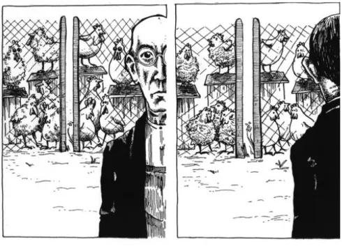
minimized. A category is simply a classificatory division. An example of perceptual warping caused by categories is illustrated below in Figure 2. Here, objects (in this case, chickens), are classified into two categories, which are represented by the two separate chicken coops. The left panel illustrates the reality of the differences of chickens. The right panel illustrates how the observer views the two categories of chickens: differences of chickens which belong to different categories are exaggerated, while differences of chickens which belong to the same category are minimized.
Figure 2. Figure taken from Goldstone and Hendrickson (2010), illustrating the effect of categories on perception: differences among objects (in this case, chickens) which fall into different categories (coops) are exaggerated, while differences among objects which fall into the same category are minimized.
17
occurs, or both across-category compression and within-category compression occur (Livingston et al., 1998; Goldstone, 1994b; Goldstone and Hendrickson, 2010; Nosofsky, 1986).
Returning to the spatial metaphor of the perceptual space, the effect that across-category expansion has on the perceptual space is to warp the perceptual space such that stimuli which belong to different categories draw apart from one another. The effect that within-category compression has on the perceptual space is to warp the perceptual space such that stimuli which belong to the same category draw nearer to one another. Therefore, the effect of learning a categorization pattern on the perceptual space is to enhance the category boundary. That is, once a participant has been trained to categorize items, the boundary between the two categories will be stretched out in the perceptual space.
Consider Figure 3 for an example of the effect of learning a categorization on the perceptual space.
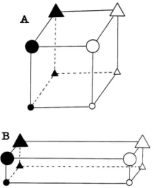
Figure 3. The effects of learning a light/dark categorization on a hypothetical participant’s perceptual space. Illustration taken from Nosofsky (1986).
18
for some hypothetical participant who has been trained to categorize the stimuli into two groups: light and dark. The effect of learning this light/dark categorization is to enhance the category boundary by both enlarging the difference between stimuli which belong to different categories (“across-category expansion,” represented in the spatial metaphor with increased distance), and shrinking the difference between stimuli which belong to the same category (“within-category compression,” represented in the spatial metaphor with decreased distance).
As mentioned above, the observation that the category boundary will become more enhanced (either through within-category compression, across-category expansion, or both) is found for stimuli from many domains, both linguistic and non-linguistic. A more enhanced category boundary following categorization training has been found for visual stimuli, auditory non-linguistic stimuli, and auditory linguistic stimuli.
In all of the examples listed below, participants were trained on some categorization pattern (“stimulus i is an X, stimulus j is a Y”). Then their perceptual spaces were inferred, either through a confusion task (more confusable pairs of stimuli fall closer to one another than less confusable pairs of stimuli in the perceptual space) or a similarity task (more similar pairs of stimuli fall closer to one another than less similar pairs of stimuli in the perceptual space)3. Experiments finding perceptual warping can be classified according to the type of stimulus used in the experiment. Visual (non-linguistic) stimuli include drawings of hypothetical
microorganisms (Livingston et al., 1998), black and white photographs of chick genitalia
(Livingston et al., 1998), drawings of rock formations (Kurtz and Gentner, 1998), equally-spaced stimuli taken from a continuum of one known face (ie. John F. Kennedy) to another well-known face (ie. Bill Clinton) (Beale and Keil, 1995), equally-spaced stimuli taken form a
continuum of novel faces on which participants were familiarized on in the lab (Levin and Beale,
19
2000), squares which varied in brightness and in size (Goldstone, 1994b), deformed ellipses (Op de Beeck et al., 2003), and colors (Winawer et al., 2007; Ӧzgen and Davies, 2002). Auditory non-linguistic stimuli include samples of white noise with different center frequencies (Guenther et al., 1999), and perception of tones by expert musicians as compared to novice musicians (Burns and Ward, 1978). Of the experiments conducted which use auditory linguistic stimuli, two effects have been found. One, named “categorical perception” (see the Note on terms #1 below, this section), describes the phenomenon in which discrimination between stimuli is much more accurate if those stimuli belong to different phonemes, as compared to stimuli which belong to the same phoneme (Liberman et al., 1957; Liberman et al., 1967). The second effect, named the Perceptual Magnet Effect, describes the phenomenon in which participants show reduced discriminability near vowel sounds which are prototypical in their native language (Kuhl, 1991). Other examples of auditory linguistic stimuli include training participants on distinguishing (“categorizing”) non-native speech contrasts. This has been done with native English participants trained to distinguish (“categorize”) the Polish alveopalatal sibilant /ɕ/ and retroflex sibilant /ʂ/ (McGuire, 2007), with native English participants trained to distinguish (“categorize”) three Korean voiceless bilabial stops, weak /p/, strong /P/, and aspirated /ph/ (Francis and Nusbaum, 2002), and with native Spanish speakers trained to distinguish (“categorize”) tense and lax English vowels (Kondaurova and Francis, 2010).
In all of the examples listed above, save that of the Francis and Nusbaum 2002 study which trained English speakers to categorize Korean voiceless bilabial stops, an enhanced category boundary was observed following categorization training, either through within-category compression, across-within-category expansion, or both.
20
were given pairs of stimuli and asked to judge the similarity of the pair using a slide-scale rating ranging from 0-100. Experimenters predicted that the similarity judgments between two stimuli which belonged to the same category (for example, two different recordings of [p]) would decrease after training, and that the similarity judgments between two stimuli which belonged to different categories (for example, [p] compared to [P]) would increase after training. Results were mixed. For the /P/ category, within-category compression and across-category expansion was found, which followed Francis and Nusbaum’s predictions. That is, the similarity judgments of [P] stimuli with other [P] stimuli increased, while similarity judgments of [P] with either [p] or [ph] decreased after training. For the /ph/ category, across-category expansion was found, but, instead of within-category compression they found decreased similarity within the /ph/ category. That is, the similarity judgments of [ph] stimuli with either [p] or [P] stimuli decreased, but the similarity judgments of [ph] stimuli with other [ph] stimuli decreased instead of increasing as predicted. Likewise for the /p/ category, across-category expansion was found, but there was decreased similarity within categories. The Francis and Nusbaum (2002) case will be discussed further in the discussion chapter.
21
(“Perceptual Magnet Effect”) are special phenomena or not, all examples covered above (with the one exception of the Francis and Nusbaum’s 2002 study, pursued further in the discussion
chapter), including that of the “categorical perception” of English stop consonants and the Perceptual Magnet Effect of vowels, are examples of an enhanced category boundary. The perceptual space around the category boundary is stretched out with respect to the perceptual space within a category.
Note on terms #1. Within psychology, within-category compression and across-category expansion (that is, better perceptual discriminability between things which belong to different categories in comparison to things which belong to the same category), is called categorical perception (Goldstone and Hendrickson, 2010). The strong version of categorical perception (within psychology) is the case where existing categories are the only criteria used to determine whether two stimuli are identical. That is, there is no ability to distinguish objects which fall into the same category.
On the other hand, within linguistics, the term categorical perception tends to refer only to this strong version (Liberman et al., 1957). Since there are few empirical examples of this strong version (Goldstone and Hendrickson, 2010), and since these examples are restricted to speech sound categories, this version of “categorical perception” is typically viewed as a language-specific property (Liberman et al., 1967; Studdert-Kennedy et al., 1970), rather than a general property of cognition.
22 2.4.1. Relevant and irrelevant dimensions
As discussed above, categories warp the perceptual space to enhance the category boundary. However, although not explicitly stated by any of the authors in the studies reviewed above, studies involving “complex” tasks, such as those involving categorizing photographs or drawings, speak of within-category compression and across-category expansion in different terms than authors of experiments which involve “simple”4 tasks, such as those involving categorizing “light” vs. “dark” squares. Authors of studies which involve “simple” tasks break stimuli down into relevant dimensions, as well as irrelevant dimensions. These will be discussed here since the present study is considered a “simple” task. The notion of relevant and irrelevant dimensions is used later to develop a measure, called a Category Ratio.
Examples of dimensions are “color,” “size,” or “shape.” A relevant dimension is a dimension which is relevant to the categorization pattern. There would be no way to correctly categorize stimuli if knowledge of the values in that dimension were not present. An irrelevant dimension is a dimension which is irrelevant to the categorization pattern. To illustrate the difference between these two, consider Figure 4.
4
23
Figure 4. Stimuli in Goldstone (1994b) experiment. Illustration taken from Goldstone and Hendrickson (2010).
Here, two dimensions can be extracted from the 16 stimuli: “brightness” and “size.” Stimuli can be arranged so that brightness increases as you move up along the brightness dimension, and size increases as you move right along the size dimension. Suppose participants are asked to
categorize stimuli into two categories: Category A and Category B. The correct category label is beneath each stimulus. As can be seen from Figure 4, all stimuli with a brightness value of “3” and “4” belong to Category A, while all stimuli with a brightness value of “1” and “2” belong to Category B. In this case, the value along the size dimension is irrelevant to a stimulus’s category membership, making the size dimension and irrelevant dimension. On the other hand, the value along the brightness dimension determines which category the stimulus falls into. Therefore the brightness dimension in this case is a relevant dimension.
24
more with the psychology “dimension.” Therefore [labial] is a dimension, while [+labial] and [-labial] are “features” according to the psychology definition. Because of this, this paper will use Goldstone’s definition of “dimension.” The term “value” will refer to what Goldstone called “feature” (ie. to things like “3 centimeters” or “red”). The term “feature” will always refer to phonological features (distinctive features), which can refer to either the value ([+labial]) or the dimension ([labial]) of a theory-dependent property of a speech sound.
For both “simple” tasks from which dimensions can be extracted and for “complex” tasks, a more enhanced category boundary is achieved. However, for “simple” tasks, it is achieved by stretching relevant dimensions (which results in across-category expansion) and shrinking irrelevant dimensions (which results in within-category compression) (Nosofsky, 1986; Goldstone, 1994b; Kruschke, 1992; Kruschke, 2011).
2.4.2. Summary of perceptual warping
To summarize, perceptual warping has been found in a variety of domains. Types of stimuli used in examples demonstrating perceptual warping can be both linguistic and non-linguistic. All examples, save for one exception (Francis and Nusbaum, 2002, pursued further in the discussion chapter), find that training participants on some categorization will result in a more enhanced category boundary. This comes in the form of within-category compression, across-category expansion, or both.
25 2.4.3. Importance for present study
The goal of the present study is to replicate Terbeek’s experiment using participants trained on an artificial language with front/back vowel harmony in place of Turkish speakers. While Terbeek’s results may have been caused by a poor fit of stimulus vowels to Turkish native vowels, it may also be caused by Turkish having front/back vowel harmony. These two possible explanations are summarized in Table 3. Hypothesis 1 states that Terbeek’s findings are no more than an error in experiment design: the stimulus vowels used in the experiment were a poor fit of Turkish native vowels. Hypothesis 2 states that Terbeek’s findings may be due in part to Turkish having front/back vowel harmony.
Hypothesis 1 Terbeek’s findings are due only to poor matching of stimulus vowels to Turkish native vowels
Hypothesis 2 Terbeek’s findings are due in part to front/back vowel harmony in Turkish
Table 3. Possible explanation for Terbeek’s finding that Turkish speakers judge front vowels as being more similar to one another compared to speakers of English, Thai, German, and Swedish, and that Turkish speakers judge back vowels as being more similar to one another compared to speakers of English, Thai, German, and Swedish.
Why should Hypothesis 2 be considered as a possible explanation? That is, why should
26
Therefore, if Hypothesis 2 is correct, we expect to see a more enhanced category boundary between front and back vowels after training English speakers on a language with front/back vowel harmony. Since this experiment uses native English speakers trained on an artificial language with front/back vowel harmony in place of Turkish speakers and since all vowels used are designed to be good matches of native English vowels, there is no possibility of any increased similarity being caused by a poor match of stimulus vowels to native vowels. Therefore, if a more enhanced category boundary is found between front and back vowels in the present experiment, Hypothesis 1 can be ruled out as a possible explanation, leaving only Hypothesis 2.
2.5. Category Ratios
As described above, different experiments found within-category compression, across-category expansion, or both. While the authors reviewed treated the difference between these three as important (see in particular Livingston et al., 1998), this experiment is more interested in whether any of these three occur, since all three have the effect of distinguishing the category boundary. This section first justifies using a new measure, which will be called a Category Ratio, and then defines this new measure. The purpose of the Category Ratio is to determine whether a category boundary has become more enhanced, following the learning of a categorization.
2.5.1. Justification for Category Ratios
27
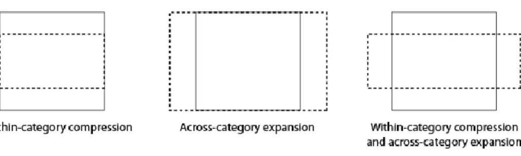
Figure 5. Three hypothetical effects of categorization on the perceptual space in which the vertical dimension is relevant to categorization. The horizontal dimension in this example is irrelevant to categorization. The solid lines indicates the perceptual space of a group which does not have a category established (ie. a control group, or a group prior to categorization training), and the dashed lines indicate a group which has a categorization which depends only on the vertical dimension.
In this example, the solid lines indicate the hypothetical perceptual space of a participant who does not have a category established (ie. a participant before categorization training or a participant who was part of the control group which received arbitrary training with no categorization pattern), and dashed lines indicate the perceptual space of a hypothetical
participant who does have a categorization established (ie. a participant who has been trained on a categorization which depends only on the vertical dimension).
28
Goldstone (1994b) trained participants to categorize squares which varied by one Just-Noticeable Difference (JND) in brightness and in size. The stimulus set consisted of 16 squares, each with one of four values of brightness and one of four values of size (see Figure 6).
Figure 6. Figure taken from Goldstone and Hendrickson (2010), illustrating the stimuli used in Goldstone (1994b). Squares vary in brightness and in size. In the example reviewed here, participants were trained to categorize squares with brightness values of “3” or “4” into Category A, and squares with brightness values of “1” and “2” into Category B.
Participants were trained to categorize squares with brightness values of “3” or “4” into Category A, and squares with brightness values of “1” and “2” into Category B. Before and after training, participants were given a pair of stimulus squares and were asked to respond whether the two squares were the same or were different. The greater ability to distinguish a pair of different squares corresponded to expansion, and the lessened ability to distinguish a pair of different squares corresponded to compression.
Given the three hypothetical effects of categorization, within-category compression, across-category expansion, or both, we would expect to find compression only within categories and expansion only across categories. However, as can be seen from the results from the
29
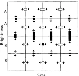
Figure 7. Results from Goldstone experiment after training participants on a categorization pattern dependent on the brightness dimension. Black rectangles with arrows indicate expansion, white rectangles with arrows indicate compression. The magnitude of the black or white rectangle indicates how much expansion or compression there was.
A more enhanced category boundary between Category A and Category B did develop, as can be seen by the large black rectangles (ie. expansion with a large magnitude) between A and B categories. However, expansion was not confined to across-category pairs. There are a few examples within-category expansion: there are a few black rectangles between Category A members, as well as a few black rectangles between Category B members.
Again, overall, the effect is that of a more enhanced category boundary. But this example shows that results will not fit in neatly with the three hypothetical examples given in Figure 5. Because of this, the measure of a Category Ratio was developed.
2.5.2. Calculation of Category Ratios
30
determined that it would be more useful to analyze all possible pairs of stimuli separately, rather than analyzing the average of all within-category distances to the average of all across-category distances in case different pairs of stimuli behaved differently (as was the case for Francis and Nusbaum (2002), in which /P/ followed all predictions, but /p/ and /ph/ did not). To do this, the notion of Category Ratios was developed.
There are two types of Category Ratios: Within-category ratios and Across-category ratios. If x and y belong to the same category, the Category Ratio of xy is a Within-category Ratio, and if x and y belong to different categories, the Category Ratio of xy is an Across-category ratio.
To conceptualize a Within-category ratio, consider the following situation:
Figure 8. Example illustrating the calculation of Within-category ratio xy. Within-category ratio xy = xy / (average (xb1,
xb2, yb3, yb4)) = 4*xy / (xb1 + xb2 + yb3 + yb4)
31
Dimension D2 and are included for reference. Possible stimuli fall at the intersection of all horizontal and vertical lines.
Since in this case the two stimuli x and y belong to the same category A, the Category Ratio of xy is a Within-category ratio. The Within-category ratio of xy in this example is the distance between x and y divided by the average of the distances between x and b1, x and b2, y and b3,and y and b4 (ie. the average of all distances indicated by the dotted lines). More generally, it is defined as the distance between x and y, divided by the average of: 1) all distances between some stimulus i and x, such that i shares the same value along the irrelevant dimension as x (value V2) and falls in a different category as x, and 2) all distances between some stimulus j and the stimulus y, such that j shares the same value along the irrelevant dimension as y (value V1) and falls in a different category from y. This can be written as follows:
32
To conceptualize Across-category ratios, consider the following example:
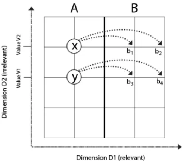
Figure 9. Example illustrating the calculation of Across-category ratio xy. Across-category ratio xy = xy / (average (xa1,
xa2, xa3, xa4, yb1, yb2, yb3, yb4)) = 8*xy / (xa1 + xa2 + xa3 + xa4 + yb1 + yb2 + yb3 + yb4)
Again, there are two categories A and B, which are determined by Dimension D1. Therefore D1 is a relevant dimension to the categorization, while D2 is not. Vertical lines indicate constant values along Dimension D1, and horizontal lines indicate constant values along Dimension D2 and are included for reference. Possible stimuli fall at the intersection of all horizontal and vertical lines.
33
that j shares the same value along the relevant dimension as y (value V2) and falls into the same category as y. This can be written more generally as follows:
for all xi such that i has the same value as x along the relevant dimension and such that i belongs to the same category as x
for all yj such that j has the same value as y along the relevant dimension and such that j belongs to the same category as y
It is expected that Within-category ratios will decrease when a category has been established, and Across-category ratios will increase.
Defining these Category Ratios also allows us to compare the results in the previously-described studies, as shown in Figures 10-185. The left column always indicates a group that does
5
Since the data given for each of the experiments above was in a different form, the Category Ratios are not applied as strictly as defined above. Specifics are described below:
Livingston et al. (1998): Category Ratios were calculated from average similarity ratings estimated from a graph. The Within-category ratio Gex-Gex was calculated as the average similarity rating of each Gex drawing with each of the other Gex drawings, divided by the average similarity rating of each Gex drawing and a Zof drawings. The Within-category ratio Zof-Zof was calculated as the average similarity rating of each Zof drawing with each of the other Zof drawings, divided by the average similarity rating of each Gex drawing and a Zof drawings. The Across-category ratio Gex-Zof was calculated as the average of each Gex drawing and a Zof drawing, divided by the average of the average similarity of Gex-Gex drawings and the average similarity of Zof-Zof drawings. Category Ratios were calculated similarly for the chick genitalia
Goldstone (1994b): Category Ratios were calculated from only a subset of the data, but were calculated as described in Section 2.5.2. Of the four brightness values and of the four size values, only the middle two of each were used in the calculation of the Category Ratios (B2, B3, S2, and S3). Category Ratios were calculated from the sensitivity index d’.
Kondaurova and Francis (2010): Category Ratios were calculated from d’ values estimated from a graph. The Within-category ratio 2-4 was calculated as the d’ value between 2-4, divided by the d’ value between 11-15. The Within-category ratio 6-8 was calculated as the d’ value between 6-8, divided by the d’ value between 11-15. The Across-category ratio was calculated as the d’ value between 11-15 divided by the average of the d’ value between 2-4 and the d’ value between 6-8. Francis and Nusbaum (2002): Category Ratios were calculated from the average similarity rating
(on a scale of 0-100). Data was given as the average similarity rating (on a scale of 0-100) of different-category pairs of X and the average distance of same-category pairs of X, where X refers to one of the three Korean stops (/P/, /p/, or /ph/).
34
not have an established category (ie. has not learned a categorization pattern, either the control group or the Pre-training results), and the right column always indicates a group that does have an established category (ie. has learned a categorization pattern, either the trained group or the Post-training results.) All dashed lines indicate Across-category ratios, and all solid lines indicate Within-category ratios. It is expected that, going from the state of no-category to existing-category, all dashed lines go up, and all solid lines go down.
Figures 10 and 11. (Top) Category Ratios calculated from similarity judgments for those not trained in any
categorization, and those trained to categorize drawings of microorganisms into “Gex” and “Zof” categories. (Bottom) Category Ratios calculated from similarity judgments for those not trained in any categorization, and those trained to categorize black and white photographs of male and female chick genitalia into categories A and B.
0 0.2 0.4 0.6 0.8 1 1.2 1.4 1.6
Control Trained
Cate go ry R ati o
Livingston et al. (1998): Drawings of microorganisms
Gex-Gex Zof-Zof Gex-Zof 0 0.2 0.4 0.6 0.8 1 1.2 1.4
Control Trained
Cate go ry R ati o
Livingston et al. (1998): Chick genitalia
A-A
B-B
35
Figures 12 and 13. (Top) Category Ratios calculated from discrimination tasks for those not trained in any
categorization, and those trained to categorize squares that differed in brightness or in size into large squares and small squares. “B3S2-B3S3” indicates the Category Ratio of the stimulus with a brightness value of 3, size value of 2, and the stimulus with a brightness value of 3 and a size value of 3. The category boundary fell between the size values S2 and S3. (Bottom) Category Ratios calculated from same-different discrimination tasks for those not trained in any categorization, and those trained to categorize squares that differed in brightness or in size into bright squares and dark squares. The category boundary fell between the brightness values B2 and B3.
0 0.2 0.4 0.6 0.8 1 1.2 1.4 1.6 1.8
Control Trained on Size
Category
Rat
io
Goldstone (1994): Squares (trained on size)
B3S2-B3S3 B2S2-B2S3 B3S2-B2S2 B3S3-B2S3 0 0.5 1 1.5 2 2.5
Control Trained on
Brightness
Category
Rat
io
Goldstone (1994): Squares (trained on brightness)
B3S2-B2S2
B3S3-B2S3
B3S2-B3S3
36
Figure 14. Spanish speakers were asked to discriminate tense and lax vowels (“sheep” vs. “ship”). Stimuli can be broken down into two dimensions: vowel duration, and spectral properties (formant measures). In the “Adaptive” training method, speakers were categorized off of a stimulus set which fixed the value of the irrelevant dimension, vowel duration, and varied only the value of the relevant dimension, spectral properties. “11-15” refers to a cross-category pair, which differs only in the spectrum dimension. “2-4” and “6-8” both refer to within-cross-category pairs, which each differ only in the duration dimension.
0 0.2 0.4 0.6 0.8 1 1.2 1.4 1.6 1.8 2
Pre Post
Category
Rat
io
Kondaurova and Francis (2010): English tense/lax vowels
11-15
2-4
37
Figures 15 and 16. (Top) Within-category ratios obtained from similarity judgments for English speakers before and after they were trained to categorize three Korean stops: strong /P/, aspirated /ph/, and weak /p/. Data was given as the average similarity rating (on a scale of 0-100) of different-category pairs of X and the average distance of same-category pairs of X, where X refers to one of the three Korean stops (/P/, /p/, or /ph/). “P” indicates the average difference of within-category pairs containing /P/ stimuli, divided by the average difference of across-category pairs containing /P/ stimuli. (Bottom) “P” indicates the average difference of across-category pairs containing /P/ stimuli, divided by the average difference of within-category pairs containing /P/ stimuli. Because of the data given, the
Within-category ratio of x is equal to the inverse of Across-category ratio of x.
As seen here, the Francis and Nusbaum (2002) case is still problematic even after the Category Ratios are applied. While the authors suggest that the unexpected expansion within categories is due to the stretching of a previously-unattended dimension, it is still unclear why there is greater
0 0.05 0.1 0.15 0.2 0.25 0.3
Pre Post
Category
Rat
io
Francis and Nusbaum (2002): Korean stops Within-category Ratios P ph p 0 5 10 15 20 25
Pre Post
Category
Rat
io
Francis and Nusbaum (2002): Korean stops Across-category Ratios
P
ph
38
expansion in the space within the /ph/ and /p/ categories than there is in the space between different categories. This is discussed further in the discussion.
Category Ratios of Terbeek’s results can also be calculated:
Figures 17 and 18. Category Ratios for a subset of the data from the Terbeek (1977) study. (Top) Within-category ratios. Example of the calculation of a Within-category ratio: ae-e / (average (ae-a + e-o)). (Bottom) Across-category ratios. Example of the calculation of an Across-category ratio: ae-a / (average((ae-e + ae-i) + (a-o + a-u))).
0 0.2 0.4 0.6 0.8 1 1.2 1.4
English Turkish
Category
Rat
io
Terbeek (1977): English vs. Turkish
Within-category Ratios for i-e-ae-u-o-a
ae-e ae-i e-i u-o u-a o-a 0 0.5 1 1.5 2 2.5 3 3.5 4 4.5 5
English Turkish
Category
Rat
io
Terbeek English vs. Turkish
Across-category Ratios for i-e-ae-u-o-a
ae-a
e-o
39
As shown in Figures 10-18, Category Ratios allow us to compare various studies. Category Ratios also allow us to determine whether or not the category boundary has been enhanced after categorization training. If a category boundary becomes more enhanced after categorization training, the Within-category ratios should decrease, and the Across-category ratios should increase. Of the five studies listed above in which Category Ratios were calculated (Figures 10-18), four of them show evidence of a more enhanced category boundary following categorization training. Only the [p] and [ph] stimuli in the Francis and Nusbaum (2002) study (pursued further in the discussion chapter) show no evidence of an enhanced category boundary.
40
CHAPTER 3
METHODS
3.1. Participants
Participants were either paid $10 for their time or were volunteers. All participants were native English speakers over the age of 18 with no history of a speech or hearing disorder. They had no background in linguistics or phonetics. When asked to list languages they had studied or were familiar with, none of them listed a language which has vowel harmony (ie. Turkish or Hungarian). Most were college undergraduates. 28 participants were assigned to the Backness group, and 26 participants were assigned to the Control group. The data from one participant from the Backness group was not included because the participant noticed and reported the front/back vowel harmony pattern in the training data, making the total 27 participants in the Backness group, and 26 in the Control group. No other participants reported noticing the front/back harmony in the after-experiment questionnaire.
3.2. Stimuli
41
ms and 225 ms respectively. The diphone used to make the second-syllable [du] contained about 45 ms of aspiration after the burst. To prevent confusion with [tu], 26 ms of the aspiration was removed. A silent interval of nominal duration 100 ms was synthesized at the beginning of the stimulus, and another of 25 ms at the end; however, the word-initial diphones contained intrinsic initial silence as well. All stimuli were 674 ms long, except those ending in [du], which were 648 ms long. No amplitude normalization was done, in order to maintain the natural amplitude difference between high and low vowels.
3.3. Procedure
The entire experiment was completed on a computer and consisted of four main parts, preceded by an instructional session and followed by a questionnaire. Participants who ran the experiment on themselves outside of the lab were instructed to wear headphones and to conduct the experiment in a quiet place. Participants who were run in the lab sat in a soundproof booth and wore headphones for the duration of the experiment.
Instructions
In the instructional session, participants were taught how to make similarity judgments. They were told they would see three circles arranged on the screen, and that they should move these circles with their mouse so that distance was inversely correlated with similarity. In other words, the more similar pairs of circles were to be placed closer together, and the less similar pairs of circles were to be placed further apart6. The three circles were all 40 pixels in diameter.
42
The initial state of the three circles was always the same: they were always arranged so that they were mostly overlapping each other and formed a small triangle. The circles were not completely overlapping so that participants could see all three circles in the initial phase, but were partially overlapping as it was thought overlapping circles would discourage participants from moving only one of the three circles if doing so would leave the remaining two very close together. When participants were finished arranging the circles, they would click a “Next” button to continue with the next triplet. Participants were unable to click the “Next” button unless they had moved at least one circle to avoid subjects accidentally double-clicking through a similarity trial. Examples of some of the instructions given to the participants can be seen in Figures 19-20.
Figure 19. Image shown in instructions. Participants were shown that the three circles would be overlapping each other in their initial state.
43
After reading the instructions, participants were given two triplets of colors to practice with (red, orange, and green; then purple, turquoise, and orange). Following this practice session,
participants were told that in the following section, the circles would now represent sounds.
Part 1: Pre-training Similarity
After practicing with colors, participants were directed to the first part of the experiment, Pre-training Similarity. They were again given three circles, but this time the circles were all the same color, and would take turns lighting up and playing one of four sounds. The order in which the circles lit up was predictable -- it always followed a clockwise-direction. Each circle within the triplet would continue to take turns lighting up and playing the sound they represented until the participant was finished moving the circles and had clicked the “Next” button. These sounds were drawn from a set consisting of [didi], [dudu], [dædæ], or [dɑdɑ] (referred to as the dVdV set). Participants were given two repetitions each consisting of the four possible combinations of triplets presented in random order ([didi dudu dɑdɑ], [didi dɑdɑ dædæ], [didi dudu dædæ], and [dudu dɑdɑ dædæ]). Within each triplet, the placement of the individual dVdV words within the triplet of circles was also random. For example, the word [didi] within the [didi dudu dɑdɑ] set might be the topmost circle in one case, and the rightmost circle or the leftmost circle in another cases. In total, participants made 8 similarity judgments (2 repetitions of 4 triplets) in Pre-training Similarity.
Part 2: Training
44
training part is the only part of the experiment which differed between the Backness group and the Control group.
Participants in the Backness group were trained on a language with front/back vowel harmony. They were given 3 repetitions of 64 “words” drawn from the language they were being trained on (total of 192 words). These 64 CVCV words were determined by taking every
combination of the four vowels [ i æ ɑ u ] allowed in that language (in other words, restricted so that only front vowels [ i æ ]or only back vowels [ɑ u ] occurred within the same word) and matching it with 8 consonant combinations: two where the consonants were the same; two where the second consonant differed only in voicing from the first consonant, two where the consonant differed only in place of articulation from the first, and two where the consonant differed in both place of articulation and voice. Table 4 shows the stimuli used in the Backness condition.
C - C C - C[voice] C - C[place] C - C[place voice]
t-t g-g k-g d-t k-t g-d t-g d-k
i-i titi gigi kigi diti kiti gidi tigi diki
i-æ titæ gigæ kigæ ditæ kitæ gidæ tigæ dikæ
æ-i tæti gægi kægi dæti kæti gædi tægi dæki
æ-æ tætæ gægæ kægæ dætæ kætæ gædæ tægæ dækæ
ɑ-ɑ tɑtɑ gɑgɑ kɑgɑ dɑtɑ kɑtɑ gɑdɑ tɑgɑ dɑkɑ
ɑ-u tɑtu gɑgu kɑgu dɑtu kɑtu gɑdu tɑgu dɑku
u-ɑ tutɑ gugɑ kugɑ dutɑ kutɑ gudɑ tugɑ dukɑ
u-u tutu gugu kugu dutu kutu gudu tugu duku
Table 4. Stimulus set for Backness group (artificial language with front/back vowel harmony).
45
C - C C - C[voice] C - C[place] C - C[place voice]
t-t g-g k-g d-t k-t g-d t-g d-k
i-i titi gigi kigi diti kiti gidi tigi diki
i-æ titæ gigæ kigæ ditæ kitæ gidæ tigæ dikæ
i-a tita giga kiga dita kita gida tiga dika
i-u titu gigu kigu ditu kitu gidu tigu diku
æ-i tæti gægi kægi dæti kæti gædi tægi dæki
æ-æ tætæ gægæ kægæ dætæ kætæ gædæ tægæ dækæ
æ-ɑ tætɑ gægɑ kægɑ dætɑ kætɑ gædɑ tægɑ dækɑ
æ-u tætu gægu kægu dætu kætu gædu tægu dæku
ɑ-i tɑti gɑgi kɑgi dɑti kɑti gɑdi tɑgi dɑki
ɑ- æ tɑtæ gɑgæ kɑgæ dɑtæ kɑtæ gɑdæ tɑgæ dɑkæ
ɑ-ɑ tɑtɑ gɑgɑ kɑgɑ dɑtɑ kɑtɑ gɑdɑ tɑgɑ dɑkɑ
ɑ-u tɑtu gɑgu kɑgu dɑtu kɑtu gɑdu tɑgu dɑku
u-i tuti gugi kugi duti kuti gudi tugi duki
u-æ tutæ gugæ kugæ dutæ kutæ gudæ tugæ dukæ
u-ɑ tutɑ gugɑ kugɑ dutɑ kutɑ gudɑ tugɑ dukɑ
u-u tutu gugu kugu dutu kutu gudu tugu duku
Table 5. Stimulus set for Control group (artificial language with no pattern within its vowels)
Part 3: Post-training Similarity
Following the training session, participants were directed to the third part of the four-part experiment, Post-training Similarity. This part was identical to Pre-training Similarity.
Part 4: Evaluation
46
“Word 2” button brought participants to the next pair of words. In all, each participant was asked to make 32 decisions. The words used in the Evaluation portion were identical for both the Backness and for the Control group.
Questionnaire
Immediately following the experiment, participants filled out a questionnaire which asked whether they had noticed any patterns in the language they had been trained on, what their language background was, and other background information.
A summary of the experiment design is seen in Table 6.
Practice Practice similarity judgments using colors 1 Pre-training Similarity
Repetition 1 using all 4 possible triplet combinations of dVdV set (i-u-a, i-u-æ, i-a-æ, u-a-æ) in random order
Repetition 2 using all 4 possible triplet combinations of dVdV set (i-u-a, i-u-æ, i-a-æ, u-a-æ) in random order
2 Training
Backness group:
Repetition 1 of 64 words in random order Repetition 2 of 64 words in random order Repetition 3 of 64 words in random order Control group:
Repetition 1 of 128 words in random order 3 Post-training Similarity
Repetition 1 using all 4 possible triplet combinations of dVdV set (i-u-a, i-u-æ, i-a-æ, u-a-æ) in random order
Repetition 2 using all 4 possible triplet combinations of dVdV set (i-u-a, i-u-æ, i-a-æ, u-a-æ) in random order
4 Evaluation