arXiv:1807.02523v1 [astro-ph.GA] 6 Jul 2018
July 10, 2018
Near infrared spectroscopy and star-formation histories
of
3
≤
z
≤
4
quiescent galaxies
⋆
C. Schreiber
1, K. Glazebrook
2, T. Nanayakkara
1,2, G. G. Kacprzak
2, I. Labbé
1,2, P. Oesch
3, T. Yuan
4, K.-V. Tran
5,6,
C. Papovich
7, L. Spitler
8,9,10, and C. Straatman
111 Leiden Observatory, Leiden University, NL-2300 RA Leiden, The Netherlands
e-mail:cschreib@strw.leidenuniv.nl
2 Centre for Astrophysics and Supercomputing, Swinburne University of Technology, Hawthorn, VIC 3122, Australia 3 Observatoire de Genève, 1290 Versoix, Switzerland
4 Research School of Astronomy and Astrophysics, The Australian National University, Cotter Road, Weston Creek, ACT 2611,
Australia
5 Australia Telescope National Facility, CSIRO Astronomy and Space Science, PO Box 76, Epping, NSW 1710, Australia 6 School of Physics, University of New South Wales, Sydney, NSW 2052, Australia
7 George P. and Cynthia W. Mitchell Institute for Fundamental Physics and Astronomy, Department of Physics and Astronomy,
Texas A&M University, College Station, TX 77843, USA
8 Research Centre for Astronomy, Astrophysics & Astrophotonics, Macquarie University, Sydney, NSW 2109, Australia 9 Department of Physics & Astronomy, Macquarie University, Sydney, NSW 2109, Australia
10 Australian Astronomical Observatory, 105 Delhi Rd., Sydney NSW 2113, Australia 11 Max-Planck Institut für Astronomie, Königstuhl 17, D-69117, Heidelberg, Germany
Received 22 March 2018; accepted 4 July 2018
ABSTRACT
We present Keck–MOSFIREHandKspectra for a sample of 24 candidate quiescent galaxies at 3 <z <4, identified from their
rest-frame UV Jcolors and photometric redshifts in the ZFOURGE and 3DHST surveys. With median integration times of one hour inHand five in K, we obtain spectroscopic redshifts for half of the sample, using either Balmer absorption lines or nebular emission lines. We confirm the high accuracy of the photometric redshifts for this spectroscopically-confirmed sample, with a median
|zphot−zspec|/(1+zspec) of 1.2%. Two galaxies turn out to be dusty Hαemitters at lower redshifts (z<2.5), and these are the only two
detected in the sub-mm with ALMA. High equivalent-width [Oiii] emission is observed in two galaxies, contributing up to 30% of the
K-band flux and mimicking theUV Jcolors of an old stellar population. This implies a failure rate of only 20% for theUV Jselection at these redshifts. Lastly, Balmer absorption features are identified in four galaxies, among the brightest of the sample, confirming the absence of OB stars. We then modeled the spectra and photometry of all quiescent galaxies with a wide range of star-formation histories. We find specific star-formation rates (sSFR) lower than 0.15 Gyr−1(a factor of ten below the main sequence) for all but one
galaxy, and lower than 0.01 Gyr−1 for half of the sample. These values are consistent with the observed Hβand [Oii] luminosities,
and the ALMA non-detections. The implied formation histories reveal that these galaxies have quenched on average 300 Myr prior to being observed, betweenz=3.5 and 5, and that half of their stars were formed byz∼5.5 with a mean SFR∼300M⊙/yr. We finally
compared theUV Jselection to a selection based instead on the sSFR, as measured from the photometry. We find that galaxies a factor of ten below the main sequence are 40% more numerous thanUV J-selected quiescent galaxies, implying that theUV Jselection is pure but incomplete. Current models fail at reproducing our observations, and underestimate either the number density of quiescent galaxies by more than an order of magnitude, or the duration of their quiescence by a factor two. Overall, these results confirm the existence of an unexpected population of quiescent galaxies atz>3, and offer the first insights on their formation histories.
Key words. Galaxies: evolution, Galaxies: high-redshift, Galaxies: statistics, Techniques: spectroscopic
1. Introduction
In the present-day Universe, clear links have been observed be-tween the stellar mass of a galaxy, the effective age of its stellar
population, its optical colors, its morphology, and its immediate environment. The most massive galaxies, in particular, tend to be located in galaxy over-densities (e.g., clusters or groups), have old stellar populations and little on-going star formation, and display red, featureless spheroidal light profiles with compact cores (e.g., Baldry et al.2004). These different observables have
⋆ Tables 3 and A.4 are available in electronic form at the CDS
via anonymous ftp tocdsarc.u-strasbg.fr (130.79.128.5) or via http://cdsweb.u-strasbg.fr/cgi-bin/qcat?J/A+A/
been used broadly to identify galaxies belonging to this popula-tion, sometimes interchangeably, and be it from their morphol-ogy [“early-type galaxies” (ETGs), “spheroids”, “ellipticals“], their colors [“red” or “red sequence galaxies”, “extremely red objects” (EROs), “luminous red galaxies” (LRGs)], their star formation history [“old”, “quiescent”, “evolved”, “passive”, or “passively evolving galaxies” (PEGs)], their mass [“massive galaxies”], their environment [“bright cluster galaxy” (BCGs), “central galaxy”], or any combination thereof.
Dun-lop et al.2007; Spitler et al.2014; Martis et al.2016). Similarly, the proportion of star-forming objects among massive galaxies, compact galaxies, or within over-dense structures was larger in the past (e.g., Butcher & Oemler1978; Elbaz et al.2007; van Dokkum et al. 2010; Brammer et al.2011; Barro et al. 2013, 2016; Wang et al.2016; Elbaz et al.2017). When exploring the evolution of galaxies through cosmic time, it is therefore cru-cial not to assume that the aforementioned observables indepen-dently map to the same population of objects, and to precisely define which population is under study.
In the present paper, we aim to constrain and understand the emergence of massive galaxies with low levels of on-going star formation, which we will dub hereafter “quiescent” galaxies (QGs), in opposition to “star-forming” galaxies (SFGs). In our view, for a galaxy to qualify as quiescent its star formation rate (SFR) needs not be strictly zero, but remain significantly lower than the average for SFGs of similar masses at the same epoch. In other words, these galaxies must reside “below” the so-called star-forming main sequence (MS, Elbaz et al.2007; Noeske et al. 2007). If found with SFRs sufficiently lower than that expected
for an MS galaxy, say below the MS by an order of magnitude or three times the observed MS scatter (e.g., Schreiber et al.2015), these galaxies must have experienced a particular event in their history which suppressed star formation (either permanently or temporarily). At any given epoch, this is equivalent to selecting galaxies with a low specific SFR (sSFR=SFR/M∗).
Regardless of how they are defined, the evolution of the num-ber density of QGs has been a long standing debate, and has proven an important tool to constrain galaxy evolution models (see Daddi et al. 2000; Glazebrook et al. 2004; Cimatti et al. 2004; Glazebrook et al.2017, discussions therein, and below). After two decades of observations, solid evidence now show that QGs already existed in significant numbers in the young Uni-verse at all epochs, now up to z ∼ 4 (e.g., Franx et al. 2003;
Glazebrook et al. 2004; Cimatti et al.2004; Kriek et al.2006, 2009; Gobat et al.2012; Hill et al.2016; Glazebrook et al.2017), and that their number density has been rising continuously until the present day (e.g., Faber et al.2007; Ilbert et al.2010; Bram-mer et al.2011; Muzzin et al.2013; Ilbert et al.2013; Stefanon et al.2013; Tomczak et al.2014; Straatman et al.2014). Spec-troscopic observations confirmed their low current SFRs from faint or absent emission lines, their old effective ages (mass- or
light-weighted) of more than half a Gyr from absorption lines, or their large masses from kinematics (e.g., Kriek et al.2006,2009; van de Sande et al. 2013; Hill et al.2016; Belli et al.2017b,a; Glazebrook et al.2017). High-resolution imaging from the Hub-ble Space Telescope(HST) simultaneously showed that distant
QGs also display “de Vaucouleurs (1948)”-type density profiles, and effective radii getting increasingly larger with time possibly
as a result of dry merging (e.g., van Dokkum et al.2008; New-man et al.2012; Muzzin et al.2012; van der Wel et al.2014b).
The existence of these galaxies in the young Universe poses a number of interesting and still unanswered questions. Chief among them is probably the fact that, according to our current understanding of cosmology, galaxies are not closed boxes but are continuously receiving additional gas from the intergalactic medium through infall (e.g., Press & Schechter1974; Audouze & Tinsley1976; Rees & Ostriker1977; White & Rees1978; Tac-coni et al.2010). While the specific infall rate should go down with time as the density contrast in the Universe sharpens and the merger rate decreases (e.g., Lacey & Cole1993), gas flows still remain large enough to sustain substantial star formation in massive galaxies, where feedback from supernovae is inefficient
(e.g., Benson et al.2003), and also in clusters (Fabian1994). A
mechanism must therefore be invoked in massive galaxies, either to remove this gas from the galaxies, or to prevent it from cool-ing down to temperatures suitable for star formation. To produce observationally-identifiable QGs, this mechanism must act over at least the lifetime of OB stars, a few tens of Myr, and should be allowed to persist over longer periods to explain their observed ages of up to several Gyrs (e.g., Kauffmann et al.2003b). This
mechanism has been dubbed “quenching” (e.g., Bower et al. 2006; Faber et al.2007).
Nowadays, the most favored actor for quenching is the feed-back that slow and fast-growing supermassive black holes can apply on their host galaxies (e.g., Silk & Rees1998; Bower et al. 2006; Croton et al.2006; Hopkins et al. 2008; Cattaneo et al. 2009). During the fastest accretion events (e.g., during a galaxy merger), the energetics of these active galactic nuclei (AGNs) is such that they are capable of driving powerful winds and re-move gas from the galaxy, resulting in so-called quasar-mode feedback. However this mechanism alone cannot prevent star formation over long periods of time. Indeed, the expelled gas eventually re-enters the galaxy. This gas must first cool down (hence form stars) before reaching the galaxy’s center, fueling black hole growth, and triggering a new quasar event. There is therefore a need to introduce a heating source to prevent the gas infalling on quiescent galaxies from cooling (this need was first identified in the core of galaxy clusters, e.g., Blanton et al.2001). This long-lasting, less violent mechanism could then maintain the quiescence established by a quasar episode.
Lower levels of accretion onto central black holes can fulfill this role, by injecting energy into the halo of their host galaxy with jets (see Croton et al.2006). However this is not the sole possible explanation. In particular, “gravitational heating” of in-falling gas in massive dark matter halos can have the same net effect (Birnboim & Dekel2003; Dekel & Birnboim2008), while
stabilization of extended gas disks by high stellar density in bulges can also prevent star formation on long timescales (Mar-tig et al.2009).
While all of these phenomena have been shown to play some role in quenching galaxies, it remains unknown which (if any) is the dominant process. For example, recent simulations show that the QG population up toz∼2 can be reproduced without the
violent feedback of AGNs and instead simply shutting offcold
gas infall, leaving existing gas to be consumed by star formation (Gabor & Davé2012; Davé et al.2017). Furthermore, the ob-servation of significant gas reservoirs in higher redshifts QGs, as well as SFGs transitioning to quiescence, suggests that quench-ing is not simply caused by a full removal of the gas, but is ac-companied (and, perhaps, driven) by a reduced star-formation ef-ficiency (e.g., Davis et al.2014; Alatalo et al.2014,2015; French et al. 2015; Schreiber et al.2016; Suess et al.2017; Lin et al. 2017; Gobat et al.2018). A complete census of QGs across cos-mic time and a better understanding of their star formation his-tories are required to differentiate these different mechanisms.
suc-cessful in the local Universe, but suffer from high contamination
at higher redshifts owing to the increasing prevalence of dusty red galaxies (e.g., Labbé et al.2005; Papovich et al.2006). Two-color criteria were later introduced to break the degeneracy be-tween dust and age to first order, and allow the construction of purer samples (Williams et al. 2009; Ilbert et al. 2010). Com-pared to full spectral modeling coupled to a more direct sSFR selection, these color criteria are less model-dependent, partic-ularly so in deep fields where the wavelength coverage is rich and interpolation errors are negligible. Because they are so sim-ple to compute, observational effects are also simpler to
under-stand. But as a trade of, the comparison with theoretical models is harder than with a more direct sSFR selection, since it requires models to predict synthetic photometry.
Recently, a number of QGs were identified atz > 3 with
such color selection technique (Straatman et al.2014; Mawatari et al.2016). Their observed number density significantly exceeds that predicted by state-of-the-art cosmological simulations, with and without AGN feedback (e.g., Wellons et al. 2015; Sparre et al.2015; Davé et al.2016), and requires a formation channel at z > 5 with SFRs larger than observed in the mostly
dust-free Lyman-break galaxies (LBGs; e.g., Smit et al.2012,2016). However, at the time the accuracy of color selections of QGs had not been tested beyondz ∼ 2, and spectroscopic confirmation
of their redshifts and properties was needed to back up these unexpected results.
For this reason, we have designed several observing cam-paigns to obtain near-infrared spectra of these color-selected
z>3 massive QGs with Keck–MOSFIRE. The first results from
this data set were described in Glazebrook et al. (2017) (here-afterG17), where we reported the spectroscopic confirmation of the most distant QG atz∼3.7, the first atz >3, using Balmer
absorption lines. While flags were raised owing to the detection of sub-millimeter emission toward this galaxy by ALMA (Simp-son et al.2017), we later demonstrated this emission originates from a neighboring dusty SFG, and provided a deep upper limit on obscured star formation in the QG (Schreiber et al.2018b). The confirmed redshift and quiescence of this galaxy (ZF-COS-20115, nicknamed “Jekyll”) provided the first definite proof that QGs do exist atz>3, and the fact that these were found in
cos-mological surveys of small area (a fraction of a square degree) implies they are not particularly rare.
In this paper, we describe the observations and results for the entire sample of galaxies observed with MOSFIRE. Using this sample, we derived statistics on the completeness and purity of theUV J color selection atz > 3, and used this information to
derive updated number densities and star formation histories for QGs at these early epochs, to compare them against models.
In section2, we describe our observations and sample, in-cluding in particular the sample selection, the spectral energy distribution (SED) modeling, and the reduction of the spectra. In section 3 we describe our methodology for the analysis of the spectra, and make an inventory of the observed spectral fea-tures, the line properties, and the measured redshifts. In partic-ular, section3.7discusses the revisedUV J colors. In section4
we discuss the quiescence and inferred star-formation histories for the galaxies with MOSFIRE spectra. In section5, we build on the results of the previous sections to update the number den-sity of quiescent galaxies, using the full ZFOURGE catalogs, and discuss the link between theUV Jselection and the specific
SFR. Lastly, section6compares our observed number densities and star formation histories to state-of-the-art galaxy evolution models, while section 7 summarizes our conclusions and lists possibilities for future works.
In the following, we assumed a ΛCDM cosmology with
H0 = 70 km s−1Mpc−1,ΩM = 0.3, ΩΛ = 0.7 and a Chabrier (2003) initial mass function (IMF) to derive physical parameters from the photometry and spectra. All magnitudes are quoted in the AB system, such thatmAB=23.9−2.5 log10(Sν[µJy]).
2. Sample selection and observations
This section describes the sample of galaxies we analyzed in this paper, the new MOSFIRE observations, the associated data re-duction, and the analysis of the spectra.
2.1. Parent catalogs
The sample studied in this paper consists of 3<z<4, massive
(M∗ ≥2×10¹⁰M⊙) galaxies identified using photometric
red-shifts. TheUV J color-color diagram was then used to separate
star-forming and quiescent galaxies (Williams et al.2009). The galaxies were selected either from the ZFOURGE or 3DHST catalogs (Skelton et al.2014; Straatman et al.2016) in the CAN-DELS fields EGS/AEGIS, GOODS–South, COSMOS, and UDS
(Grogin et al.2011; Koekemoer et al.2011). All fields include a wide variety of broadband imaging ranging from theU band
up to theSpitzer8µm channel. This includes in particular (5σ
limiting magnitudes quoted for EGS, GOODS-S, COSMOS, and UDS, respectively): deep Hubble imaging in the F606W
(R < 26.8, 27.4, 26.7, 26.8); F814W (I < 26.4, 27.2, 26.5,
26.8); F125W (J <26.3, 26.1, 26.1, 25.8); F160W (H <26.1,
26.4, 25.8, 25.9); deepKsorK-band imaging (K<24, 24.8, 25,
24.9); and deepSpitzer3.6 and 4.5µm imaging ([3.6] < 25.2,
24.8, 25.1, 24.6). The photometry in these catalogs was assem-bled with the same tools and approaches, namely aperture pho-tometry on residual images cleaned of neighboring sources (see Skelton et al.2014; Straatman et al.2016).
The ZFOURGE catalogs supersede the 3DHST catalogs by bringing in additional medium bands fromλ=1.05 to 1.70µm
and deeper imaging in theKs band (obtained with the
Magel-lan FourStar camera). The additional near-infrared filters allow a finer sampling of the Balmer break atz∼2–3, and more
accu-rate photometric redshifts. However, they only cover a 11′×11′
region within each of the southern CANDELS fields (GOODS– South, UDS, and COSMOS). We thus used the higher quality data from ZFOURGE whenever possible, and resorted to the 3DHST catalogs outside of the ZFOURGE area. In both cases, we only used galaxies with a flag use=1. In ZFOURGE, we
used an older version of theuseflags than that provided in the
DR1. Indeed, the latter were defined to be most conservative, in that they flag all galaxies which are not covered in all FourStar bands, those missingHST imaging, or those too close to star
spikes in optical ground-based imaging (Straatman et al.2016). This would effectively reduce the covered sky area by excluding
galaxies which, albeit missing a few photometric bands, are oth-erwise well characterized. Instead, we adopted the earlieruse
flags from Straatman et al. (2014), which are more inclusive. After the sample was assembled, a few source-specific ad-justments were applied to the catalog fluxes. For ZF-COS-17779, we discarded the CFHT photometry which had nega-tive fluxes with high significance (although inspecting the im-ages did not uncover any particular issue). For 3D-EGS-26047 we removed the WirCAMJband which was incompatible with
the flux in the surrounding passbands (including the NewfirmJ
Table 1: List of model parameters in our SED modeling.
Parameter (unit) Low Up Step Values
tburst(Gyr) 0.01 tH(z) 0.05a 45–50
τrise(Gyr) 0.01 3 0.1a 26
τdecl(Gyr) 0.01 3 0.1a 26
RSFR 10−2 105 0.2a 36
tfree(Myr) 10 300 0.5a 4
AV(mag) 0 6 0.02 61
Z Z⊙
z zphotorzspec
IMF Chabrier (2003)
Attenuation curve Calzetti et al. (2000) Stellar population Bruzual & Charlot (2003)
aLogarithmic step, in dex.
the noise in the image at this location is higher but the error bars reported in the catalog were severely underestimated, visual in-spection of the image revealed no detection. For 3D-EGS-31322, we removed theSpitzer5.8 and 8µm fluxes which were
abnor-mally low; the galaxy is located in a crowded region, and the photometry in these bands may have been poorly de-blended. These modifications are minor, and do not impact our results sig-nificantly. Lastly, for ZF-COS-20115 (theG17galaxy) we used the photometry derived in Schreiber et al. (2018b), where the contamination from a dusty neighbor (Hyde) was removed. This
reduced the stellar mass of ZF-COS-20115 by 30% and had no impact on its inferred star formation history (see Schreiber et al. 2018b).
In this paper, our main focus is placed on quiescent galax-ies observed with MOSFIRE (this sample is described later in section 2.4). However, to place these galaxies in a wider context, we also considered all massive galaxies in the parent sample at 3 < z < 4. For this purpose, we only used the
ZFOURGE catalogs (in GOODS–South, COSMOS, and UDS) since they have data of similarly high quality, and are all Ks
-selected (while the 3DHST catalogs were built from a detection image in F125W+F140W+F160W). To further ensure reliable
photometry, we only considered galaxies with Ks < 24.5; the
impact of this magnitude cut on the completeness is addressed in the next section. We visually inspected the SEDs and images of all galaxies withM∗>1010M⊙to reject those with
problem-atic photometry (3% of the inspected galaxies). In the end, the covered area was 139, 150, and 153 arcmin2in GOODS–South,
COSMOS, and UDS, respectively.
2.2. Initial photometric redshifts and galaxy properties
The photometric redshifts (zphot), rest-frame colors (U−V and
V − J), and stellar masses (M∗) provided in the ZFOURGE
and 3DHST catalogs were computed with the same softwares, namely EAzY (Brammer et al. 2008) and FAST (Kriek et al. 2009), albeit with slightly different input parameters. These
val-ues were used to build the MOSFIRE masks in the different
ob-serving programs. However, to ensure the most homogeneous data set for our analysis, we recomputed redshifts, colors, and masses for all galaxies once the sample was compiled, using a uniform setup for all fields and taking advantage of all the avail-able photometry. This setup is described below.
main formation phase quenched phase
tform <SFR>
tquench
RSFR=1:
RSFR=100:
2.5 2.0 1.5 1.0 0.5 0.0
tobs − t [Gyr]
SFR(t)
tfree tburst
τdecl
τrise
RSFR
Big Bang
Fig. 1: Illustration of the adopted star formation history parametrization (bottom) and the marginalized parameters (mid-dle and top). We show the time of peak SFR (solid gray line, here coinciding withtburst), the star-forming phase surrounding
it (shaded in pale blue), and the mean SFR during this phase (horizontal blue dotted line). We also display the time of quench-ingtquench(orange solid line) and the following quenched phase
(shaded in pale orange). Finally, the time at which the galaxy had formed 50% its stars (tform) is shown with a blue solid line.
Photometric redshifts and rest-frame colors were obtained with the latest version of EAzY1 and the galaxy template set
“eazy_v1.3”, which includes in particular a “old and dusty”
and a “high-equivalent-width emission line” template. These ad-ditional templates were also used in the original ZFOURGE cat-alogs, but not in 3DHST. We also did not enable the redshift prior based on theK-band magnitude since this prior is based on
models which do not reproduce the high redshift mass functions (see discussion in section6). The resulting scatter in photomet-ric redshifts was 5% when comparing our new redshifts to that published by ZFOURGE for the entire catalog atz>3, and 7%
for the quiescent galaxies (described later in section2.4). Stellar masses and SFRs were re-computed using FAST++2
v1.2 with the same setup as in Schreiber et al. (2018b), but with more refined star-formation histories. Briefly, we assumed
z=zphot, the Bruzual & Charlot (2003) stellar population model,
the Chabrier (2003) initial mass function (IMF), and the dust screen model of Calzetti et al. (2000) with AV up to 6 mag.
The only notable difference with the published ZFOURGE and
3DHST catalogs is that we assumed a more elaborate functional
1 Commit #5590c4a (19/12/2017) on
https://github.com/gbrammer/eazy-photoz.
form for the star formation history (SFH), which consisted of two main phases: an exponentially rising phase followed by an exponentially declining phase, both with variablee-folding times τriseandτdecl, respectively:
SFRbase(t)∝
(
e(tburst−t)/τrise fort>t
burst,
e(t−tburst)/τdecl fort
≤tburst, (1)
wheretis the “lookback” time (t =0 is the point in time when
the galaxy is observed, t > 0 is in the galaxy’s past). This
was performed assuming z = zphot initially, and later on with
z=zspec(section4.1). Varying the lookback timetburstthat
sep-arates these two epochs, this allowed us to describe a large va-riety of SFHs, including rapidly or slowly rising SFHs, constant SFHs, and rapidly or slowly quenched SFHs (see Schreiber et al. 2018bfor a more detailed description of this model). Allowing rising SFHs in particular can prove crucial to properly charac-terize massive SFGs at high redshift (Papovich et al.2011). We variedtburstfrom 10 Myr to the age of the Universe (at most 2 Gyr
atz>3), andτriseandτdeclfrom 10 Myr to 3 Gyr, all with
loga-rithmic steps (0.05 dex fortburst, 0.1 dex forτriseandτdecl).
In addition, following Ciesla et al. (2016,2017) andG17, we decoupled the current SFR from the past history of the galaxy by introducing a free multiplicative factor to the instantaneous SFR within a short period, of lengthtfree, preceding observation:
SFR(t)=SFRbase(t)×
( 1 for
t>tfree,
RSFR fort≤tfree. (2)
We considered values oftfree ranging from 10 to 300 Myr, and
values of RSFR ranging from 10−2 to 105 (i.e., either abrupt
quenching or bursting), with logarithmic steps of 0.5 and 0.2 dex,
respectively. We emphasize that this additional parameter is not directly linked to quenching, as a galaxy may still have a very low sSFR from Eq.1 alone (see Fig. 1). In fact, as discussed later in section4.2, this additional freedom had little impact on the quiescent galaxies beside marginally increasing the uncer-tainty on the SFH, however we find it is necessary to properly reproduce the bulk properties of the star-forming galaxies. In particular, without this extra freedom the mean sSFR of main-sequence galaxies was too low by a factor of about three com-pared to stackedHerscheland ALMA measurements (this is also
an issue affecting the SFRs provided in the original ZFOURGE
and 3DHST catalogs).
This model is illustrated in Fig.1, and the parameters with their respective bounds are listed in Table 1. Over 200 mil-lion models were considered for each galaxy, and the fit could be performed on a regular desktop machine in less than a day thanks to the numerous optimizations in FAST++. The adopted
parametrization described above may seem overly complex, and indeed most of the free parameters in Eqs. 1 and2have little chance to be constrained accurately. This was not our goal how-ever, since we eventually marginalized over all these parameters to compute more meaningful quantities, such as the current SFR and stellar mass, and non-parametric quantities describing the SFH (see Fig.1and section4.1). The point of introducing such complexity is therefore to allow significant freedom on the SFH, to avoid forcing too strong links between the current and past SFR, as well as to obtain accurate error bars on the aforemen-tioned quantities. A similar approach was adopted inG17.
We then compared our best-fit values to that initially given in the ZFOURGE and 3DHST catalogs. Considering all galaxies at 3 <zphot <4 andM∗ >1010M⊙, we find a scatter in stellar
masses of 0.07 dex with a median increase of+0.04 dex (our new
masses are slightly larger), while the scatter in SFR is 0.34 dex
and a median increase of+0.26 dex (our SFRs are substantially
larger).
To estimate the completeness in mass of our sample result-ing from our Ks < 24.5 magnitude cut, we binned galaxies
in sSFR and computed in each bin the 80th percentile of the mass-to-light ratio inK,hM∗/LKi (whereLK is the luminosity in the observedKs band andM∗is the best-fit stellar mass
ob-tained with FAST++). We note that this method accounts for
changes inM/Lcaused both by variations in stellar populations
as well as variation in dust obscuration. Since galaxies with low sSFR tend to be less obscured at fixed mass (Wuyts et al. 2011), these two effects work in opposite directions and can lead
to a weaker evolution ofM/Lwith sSFR. In practice, we find hM∗/LKi=1.6M⊙/L⊙for sSFR=10−3Gyr−1, and 0.24M⊙/L⊙
for sSFR=10 Gyr−1. Our adopted magnitude cut ofKs <24.5
impliesM∗>2.3×10¹⁰ hM∗/LKiatz=3.5, hence a 80% com-pleteness down to 3.7×10¹⁰M⊙for sSFR<10−3Gyr−1(this is
consistent with the value obtained in Straatman et al.2014), and a factor seven lower at sSFR=10 Gyr−1.
2.3. MOSFIRE masks and runs
MOSFIRE (McLean et al.2012) is a multi-object infrared spec-trograph installed on the Keck I telescope, on top of Mauna Kea in Hawaii. Its field of view of 6′×3′can be used to
simultane-ously observe up to 46 slits per mask, with a resolving power ofR ∼ 3500 in a single band ranging fromY (0.97µm) to K
(2.41µm). The data presented here make use only of theHand Kbands.
The quiescent galaxies studied in this paper were observed by four separate MOSFIRE programs comprising 10 different
masks, listed in Table2. All masks contained a bright “slit star”, detected in each exposure, which was used a posteriori to mea-sure the variations of seeing, alignment, and effective
transmis-sion with time (see AppendixB). Slits were configured with the same width of 0.7′′ (except for the mask COS-Y259-A which
had 0.9′′ slits), and masks were observed with the standard
“ABBA” pattern, nodding along the slit by±1.5′′around the
tar-get position. Individual exposures lasted 120 and 180s in theH
andKbands, respectively.
The first program was primarily targetingz∼3.5 quiescent
galaxies (PI: Glazebrook), and observed one mask in EGS, one mask in COSMOS, and one mask in UDS (masks COS-W182, UDS-W182, and EGS-W057). Each mask was observed in the
H andK filters, with on-source integration times ranging from
0.3 to 3.9 hours in H, and 2.4 to 7.2 hours in K. The masks
were filled in priority with quiescent galaxy candidates iden-tified in Straatman et al. (2014) (or from the 3DHST catalogs for EGS), and our MOSFIRE observations for the brightest of these galaxies were already discussed in G17. The remaining slits were filled with massivez ∼ 4 star-forming galaxies, and z∼2 galaxies; these fillers are not discussed in the present
pa-per, and were only used for alignment correction and data quality tests. The SEDs of all galaxies were visually inspected, and this determined their relative priorities in the mask design.
The second and third programs (PIs: Oesch, Illingworth) were more broadly targeting massive galaxies at 2 < z < 3.6
identified in the 3DHST catalogs, and quiescent galaxies were not prioritized over star-forming ones (see van Dokkum et al. 2015). These programs consisted of multiple masks in EGS, COSMOS and UDS, however all the quiescent candidates in EGS were atz<3. We thus only used a total of three masks in
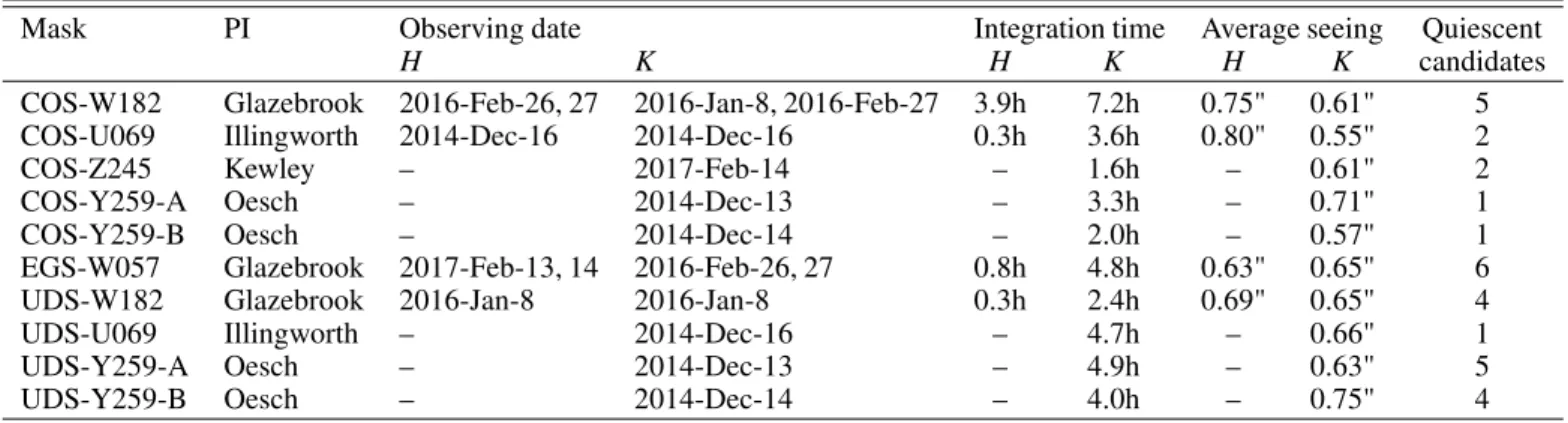
UDS-Table 2: MOSFIRE masks used in this paper.
Mask PI Observing date Integration time Average seeing Quiescent
H K H K H K candidates
COS-W182 Glazebrook 2016-Feb-26, 27 2016-Jan-8, 2016-Feb-27 3.9h 7.2h 0.75" 0.61" 5
COS-U069 Illingworth 2014-Dec-16 2014-Dec-16 0.3h 3.6h 0.80" 0.55" 2
COS-Z245 Kewley – 2017-Feb-14 – 1.6h – 0.61" 2
COS-Y259-A Oesch – 2014-Dec-13 – 3.3h – 0.71" 1
COS-Y259-B Oesch – 2014-Dec-14 – 2.0h – 0.57" 1
EGS-W057 Glazebrook 2017-Feb-13, 14 2016-Feb-26, 27 0.8h 4.8h 0.63" 0.65" 6
UDS-W182 Glazebrook 2016-Jan-8 2016-Jan-8 0.3h 2.4h 0.69" 0.65" 4
UDS-U069 Illingworth – 2014-Dec-16 – 4.7h – 0.66" 1
UDS-Y259-A Oesch – 2014-Dec-13 – 4.9h – 0.63" 5
UDS-Y259-B Oesch – 2014-Dec-14 – 4.0h – 0.75" 4
U069). Only one mask was observed in the H band for 0.3h,
and all masks were observed inKwith integration times ranging
from 2.0 to 4.9h.
The fourth and last program is the MOSEL emission line survey (PI: Kewley). This program observed several masks, in which massivez ∼ 4 galaxies from ZFOURGE were only
ob-served as fillers. Only two quiescent galaxy candidates were ac-tually observed in one mask of the COSMOS field (mask COS-Z245), where 1.6h was spent observing in the K band. One of
them was the galaxy described inG17, for which the red end of theKwas observed to cover the absent [Oiii] emission line.
2.4. Observed sample
From the MOSFIRE masks described in the previous section, we extracted all the galaxies withzphot>2.8,M∗≥2×10¹⁰M⊙
andUV J colors satisfying the Williams et al. (2009) criterion
with a tolerance threshold of 0.2 mag. The resulting 24 quiescent
galaxy candidates are listed in Table A.1, and their properties determined from the photometry alone (section2.2) are listed in TableA.2. The photometric redshifts ranged fromzphot = 2.89
up to 3.91, and stellar masses ranged fromM∗ =2.3×10¹⁰to
4.5×10¹¹M⊙, as illustrated in Fig.2. The broadband SEDs and
best fit models usingzphotare shown in Fig.3.
Some of our targets were observed in multiple MOSFIRE masks, and have accumulated more exposure time than the rest of the sample. In particular, ZF-COS-20115 (already described inG17) was observed for a total of 14.4h in theKband and 4.2h
inH. Other galaxies have exposure times ranging from 1.6h to
7.3h in theK band, and zero to 3.9h in H. The resulting line
sensitivities are discussed in section2.7.
In Fig. 2 we compare this sample to recent spectroscopic campaigns targeting high-redshift galaxies. With the exception of the sample studied in Marsan et al. (2017), massive galaxies atz>3 have so far received very limited spectroscopic coverage,
and the situation is even worse for quiescent galaxies. Priority is often given to lower mass, bluer galaxies, for which redshifts can be more easily obtained with emission lines. Indeed, we checked that, despite being selected in the well studied CANDELS fields, none of our targets were observed by the largest spectroscopic programs (MOSDEF, VUDS, and VANDELS). The only excep-tion is ZF-COS-20115 which was observed by MOSDEF for 1.6h inK; we did not attempt to combine these data with our
own given that this galaxy was already observed for 14 hours
and such a small increment would not bring significant improve-ment.
Combining data from these different programs, the collected
MOSFIRE data have a non-trivial selection function. In some programs, galaxies were prioritized based on how clean their SEDs looked, which can bias our sample toward those quies-cent candidates with the best photometry, or those with a more pronounced Balmer break. In addition, samples drawn from the 3DHST catalogs also tend to have lower redshifts and brighter magnitudes than that drawn from the ZFOURGE catalogs, as could be expected based on the different selection bands and
depths in these two catalogs. Yet, as shown in Fig.4, the com-bined sample does homogeneously cover the magnitude-redshift or mass-redshift space for quiescent galaxies, within 3<z<4
andM∗ >4×10¹⁰M⊙(orK < 23.5). We thus considered this
spectroscopic sample to be fairly representative of the overall
UV J-quiescent population at these redshifts.
2.5. Reduction of the spectra
The reduction of the raw frames into 2D spectra was performed using the MOSFIRE pipeline as in Nanayakkara et al. (2016). However, since we were mostly interested in faint continuum emission, we performed additional steps in the reduction to im-prove the signal-to-noise and the correction for telluric absorp-tion. The full procedure is described in AppendixB, and can be summarized as follows.
All masks were observed with a series of standard ABBA exposures, nodding along the slit. For each target, rather than stacking all these exposures into a combined 2D spectrum, we reduced all the individual “A−B” exposures separately and
ex-tracted a 1D spectrum for each pair of exposures. These spec-tra were optimally exspec-tracted with a Gaussian profile of width determined by the time-dependent seeing (hence, assuming the galaxies are unresolved), and were individually corrected for tel-luric correction and effective transmission using the slit star.
z 8
9 10 11 12
log
10
M
*
[M
•O
]
2.0 2.5 3.0 3.5 4.0 4.5
1.5 2
2.5 3
age of Universe [Gyr]
Kriek+06,09,16 van de Sande+13 van Dokkum+15 Kado-Fong+17 Belli+14,17 Marsan+17
this work (zphot)
Kriek+06,09,16 van de Sande+13 van Dokkum+15 Kado-Fong+17 Belli+14,17 Marsan+17
this work (zphot)
ZFIRE MUSE VANDELS VUDS MOSDEF Onodera+16
ZFIRE MUSE VANDELS VUDS MOSDEF Onodera+16
-0.5 0.0 0.5 1.0 1.5 2.0
(V-J)rest,AB 0.0
0.5 1.0 1.5 2.0 2.5
(U-V)
rest,AB
z > 3 and log10 M* > 10 Q SF
Fig. 2:Left:Stellar mass as a function of redshift for galaxies with public spectroscopic redshifts from the literature (circles) and galaxies from our sample with photometric redshifts (red stars, using photometric redshifts). We show the sample of massivez>3
galaxies from Marsan et al. (2017) in dark blue, the sample of Onodera et al. (2016) in light blue, the quiescentz ∼ 2 galaxies
of Belli et al. (2014,2017a) in dark green and Kado-Fong et al. (2017) in orange, the compactz∼2 star-forming galaxies of van
Dokkum et al. (2015) in pink, the quiescent galaxies observed in Kriek et al. (2006,2009,2016) in medium blue, the quiescent galaxies from van de Sande et al. (2013) in black, the galaxies observed by MOSDEF (Kriek et al.2015) in orange, the galaxies observed by VUDS (Tasca et al.2017) in green, the galaxies observed by VANDELS (McLure et al.2017) in purple, the galaxies in the MUSE deep fields (Inami et al.2017) in light pink, and the targets of the ZFIRE program in gray (Nanayakkara et al.2016). Right:UV J color-color diagram for a subset of galaxies shown on the left, limited toz>3 andM∗ >1010M⊙. The (U−V) and
(V −J) colors were computed in the rest frame, in the AB system. The black line delineates the standard dividing line between
quiescent (Q) and star-forming (SF) galaxies, as defined in Williams et al. (2009).
by bootstrapping the exposures, and a binning of three spec-tral elements was adopted to avoid specspec-trally-correlated noise. This resulted in an average dispersion ofλ/∆λ∼3000, which is
close to the nominal resolution of MOSFIRE with 0.7′′slits.
Fur-ther binning or smoothing were used for diagnostic and display purposes, but all the science analysis was performed on these
λ/∆λ ∼ 3000 spectra. For this and in all that follows, binning
was performed with inverse variance weighting, in which regions of strong OH line residuals were given zero weight.
2.6. Rescaling to total flux
Our procedure for the transmission correction includes the flux calibration, as well as slit loss correction. However, because the star used for the flux calibration is a point source, the slit loss corrections are only valid if our science targets are also point-like (angular size≪0.6′′, the typical seeing, see Table2). If not,
additional flux is lost outside of the slit and has to be accounted for.
We estimated this additional flux loss by analyzing the
H and K broadband images of our targets, convolved with a
Gaussian kernel if necessary to match our average seeing (see Nanayakkara et al.2016). We simulated the effect of the slit by
measuring the broadband fluxSslitin a rectangular aperture
cen-tered on each target and with the same position angle as in the MOSFIRE mask, and by measuring the “total” flux in a 2′′
di-ameter aperture,Stot. Since our transmission correction already
accounted for slit loss for a point source, we also measured the fraction of the flux in the slit for a Gaussian profile of width equal to the seeing, fPSF,slit. We then computed the expected slit
loss correction for extended emission asStot×fPSF,slit/Sslit. The
obtained values ranged from 1.0 (no correction) to 1.8 with a
median of 1.2, and were multiplied to the 1D spectra.
We then compared the broadband fluxes from the ZFOURGE or 3DHST catalogs against synthetic fluxes generated from our spectra, integrating flux within the filter response curve of the corresponding broadband. Selecting targets which have a syn-thetic broadband flux detected at>10σ, we find that our
correc-tions missed no more than 30% of the total flux, with an average of 10%. For fainter targets, this number reached at most 150%, and the highest values are found for the three faintest targets of the EGS-W057 mask (EGS-26047, EGS-27584 and 3D-EGS-34322). While one of these three is intrinsically faint and thus has an uncertain total flux, the other two were expected to be detected with a synthetic broadbandS/N of 19 and 25, but
we find only 9 and 7, respectively. This may suggest a misalign-ment of the slits for these particular targets. To account for this and other residual flux loss, we finally rescaled all our spectra to match the ZFOURGE or 3DHST photometry. We only per-formed this correction if the continuum was detected at more than 5σin the spectrum, to avoid introducing additional noise.
We noted that one galaxy’s average flux in theHband was
0.0 0.2 0.4 0.6 0.8 1.0 1.2 1.4 Sλ [10 −19 cgs]
ZF−COS−20133 zphot=3.508
zspec=3.481
0.0 0.5 1.0 1.5
2.0 ZF−UDS−3651 zphot=3.870
0.0 0.2 0.4 0.6 0.8 1.0
ZF−COS−17779 zphot=3.912
zspec=3.415
0 2 4 6
3D−EGS−18996 zphot=2.989
zspec=3.239
0.0 0.5 1.0 1.5 2.0 Sλ [10 −19 cgs]
ZF−COS−18842 zphot=3.468
zspec=3.782
0.0 0.5 1.0 1.5
ZF−UDS−4347 zphot=3.576
0.0 0.5 1.0
1.5 ZF−UDS−8197 z phot=3.470
zspec=3.543
0.0 0.5 1.0 1.5 2.0
2.5 ZF−UDS−6496 zphot=3.497
0.0 0.2 0.4 0.6 0.8 Sλ [10 −19 cgs]
3D−UDS−35168 zphot=3.461
0.0 0.5 1.0 1.5 2.0 2.5
3.0 ZF−COS−14907 zphot=2.885
0.0 0.2 0.4 0.6 0.8 1.0 1.2
1.4 3D−EGS−34322 zphot=3.586
0 1 2
3 3D−EGS−26047 zphot=3.236
zspec=3.234
0.0 0.2 0.4 0.6 Sλ [10 −19 cgs]
ZF−COS−10559 zphot=3.342
0 1 2 3
4 3D−EGS−31322 zphot=3.471
zspec=3.434
0.0 0.5 1.0 1.5
2.0 ZF−UDS−7542 zphot=3.152
0.0 0.2 0.4 0.6 0.8 1.0 1.2
1.4 3D−UDS−39102 zphot=3.513
0 2 4 6 Sλ [10 −19 cgs]
3D−EGS−40032 zphot=3.216
zspec=3.219
0 1 2 3 4 5
6 3D−UDS−41232 zphot=3.013
0.0 0.2 0.4 0.6 0.8 1.0
1.2 ZF−COS−19589 zphot=3.732
zspec=3.715
0.0 0.5 1.0
1.5 3D−UDS−27939 zphot=3.216
zspec=2.210
1 10
observed wavelength [µm]
0.0 0.5 1.0 1.5 2.0 2.5 3.0 Sλ [10 −19 cgs]
ZF−COS−20115 zphot=3.641
zspec=3.715
1 10
observed wavelength [µm]
0.0 0.5 1.0 1.5 2.0 2.5
3.0 ZF−UDS−7329 zphot=3.042
1 10
observed wavelength [µm]
0 1 2 3
4 3D−EGS−27584 zphot=3.603
1 10
observed wavelength [µm]
0.0 0.5 1.0
1.5 ZF−COS−20032 zphot=3.547
zspec=2.474
Fig. 3: Spectral energy distributions of the galaxies in our target sample, sorted by increasing observer-framez−Kcolor (rest-frame
NUV−gatz =3.5). The observed photometry is shown with open black squares and gray error bars, and the best-fitting stellar
continuum template from FAST++obtained assumingz=zphotis shown in gray in the background. For galaxies with a measured
spectroscopic redshift (see section3.3), we display the best-fitting template atz=zspecin orange, and the photometry corrected for
emission line contamination with red squares.
(1.5′′) to a brightz∼1 galaxy, we suspect that some of the bright
galaxy’s flux contaminated theHband. Regardless of the cause,
thisH-band spectrum was unusable. However, and perhaps
ow-ing to the neighborow-ing galaxy beow-ing fainter in K, the K-band
spectrum appeared unaffected and the target galaxy’s continuum
was well detected; we thus kept it in our sample and simply dis-carded theH-band spectrum.
2.7. Achieved sensitivities
The achieved spectral sensitivities andS/Nin coarse 70 Å bins
(∼1000 km/s) are listed for all our targets in Table A.3. We
2.8 3.0 3.2 3.4 3.6 3.8 4.0 zphot
25 24 23 22 21 20
KAB
10.5 11.0 11.5 ZFOURGE
3DHST MOSFIRE targets
Fig. 4: K-band magnitude as a function of photometric
red-shift for UV J quiescent galaxies (with a 0.2 mag threshold on
theUV Jdiagram). The quiescent galaxies from ZFOURGE are
shown in red, while those from 3DHST in UDS and EGS are shown in orange. The stars indicate the galaxies for which we collected MOSFIRE spectra. The red arrow indicates the po-sition of thez = 3.7 galaxy first discussed in G17. The gray
solid lines show theK-band magnitude corresponding to diff
er-ent stellar masses, 3×10¹⁰, 1011, and 3
×1011M⊙ (assuming M∗/LK=M⊙/L⊙).
the average sensitivity can vary from one galaxy to the next. In practice, the median sensitivity (1σ, [min, median, max])
ranges between [0.4,0.7,0.9]×10−19erg/s/cm2/Å inH band,
and [0.2,0.5,0.9]×10−19erg/s/cm2/Å inK, which resulted in
continuumS/N of [0.4,1.3,7.1] and [0.7,3.6,12], respectively
(these ranges reflect variation within our sample, and not varia-tions of sensitivity within a given spectrum).
In terms of line luminosity at z = 3.5, assuming a width
of σ = 300 km/s, these correspond to 3σ detection limits
of [0.5,0.9,1.1]×1042erg/s in H band, and [0.3,0.6,1.1]×
1042erg/s/cm2/Å in K. For Hβ in K and assuming no dust
obscuration, this translates into 3σ limits on the SFR of
[4,9,16]M⊙/yr (see section 4.3 for the conversion to SFR).
For the massive galaxies in our sample, this is a factor [0.04,0.11,0.20] times the main sequence SFR. With AV = 2 mag, this is increased to a factor [0.39,0.98,1.8]. Therefore,
on average, our spectra are deep enough to detect low levels of unobscured star-formation, or obscured star-formation in main-sequence galaxies.
Finally, given the observed K-band magnitudes of our
targets and considering the median uncertainties listed above, these spectra allow us to detect lines contribut-ing at least [0.3,1.1,3.8]% of the observed broadband flux (resp. [min,median,max] of our sample). This suggests we should be able to determine, in all our targets, if emission lines contribute significantly to their observed Balmer breaks. How-ever this is assuming a constant uncertainty over the entire
K band, which is optimistic. Indeed, a fraction of the
wave-length range covered by the MOSFIRE spectra is rendered un-exploitable because of bright sky line residuals.
To quantify this effect for each galaxy, we set up a line
de-tection experiment in which we simulated the dede-tection of a sin-gle line, of which we varied the full width from∆λ = 100 to
1000 km/s, and the central wavelengthλ0within the boundaries
of the K filter passband. In each case, we computed the line
flux required for the line to contribute f =10% to the observed
broadband flux, accounting for the broadband filter transmission at the line’s central wavelength. For simplicity, here we assume that the line has a tophat velocity profile and that the filter re-sponse does not vary over the wavelength extents of the line. By definition,
SBB=
R
dλR(λ)Sλ(λ) R
dλR(λ) (3)
where SBB is the observed broadband flux density (e.g., in
erg/s/cm2/Å),R(λ) is the broadband filter response, andSλ(λ)
is the spectral energy distribution of the galaxy. Decomposing
Sλinto a line and a continuum components, and with the above
assumptions, we can extract the line peak flux density
Sline(f, λ0,∆λ)= f SBB
R
dλR(λ)
∆λR(λ0) . (4)
For each galaxy, we then compared this line flux against the observed error spectrum, and computed the fraction of the
K passband where such a line could be detected at more than
5σsignificance. At fixed integrated flux, narrower lines should
have a higher peak flux and thus be easier to detect, but they can also totally overlap with a sky line and become practically unde-tectable, contrary to broader lines. As we show below, in practice these two effects compensate such that the line detection
proba-bility does not depend much on the line width.
We find that narrow lines (100 km/s) can be detected over
[73,82,92]% of the K passband, while broad lines (500 km/s)
can be detected over [77,86,96]% (resp. [min,median,max] of our sample). Therefore the probability of missing a bright emis-sion line, which we adopted as the average probability for the narrow and broad lines, is typically 15% per galaxy. The high-est value is 27% (3D-UDS-35168) and is in fact more caused by lack of overall sensitivity toward the red end of theK band
rather than by sky lines. We used these numbers later on, when estimating detection rates, by attributing a probability of missed emission line to each galaxy.
2.8. Archival ALMA observations
We cross matched our sample of quiescent galaxies with the ALMA archive and find that nine galaxies were observed, all in Band 7 except ZF-COS-20115 which was also observed in Band 8. The majority (COS-10559, COS-20032, ZF-COS-20115, ZF-UDS-3651, ZF-UDS-4347, ZF-UDS-6496, and 3D-UDS-39102) were observed as part of the ALMA program 2013.1.01292.S (PI: Leiton), which we introduced in Schreiber et al. (2017). ZF-COS-20115 was also observed in Band 8 in 2015.A.00026.S (PI: Schreiber; Schreiber et al. 2018b), ZF-UDS-6496 was also observed in 2015.1.01528.S (PI: Smail), while 3D-UDS-27939 and 3D-UDS-41232 were observed in 2015.1.01074.S (PI: Inami).
We measured the peak fluxes of all galaxies on the primary-beam-corrected ALMA images, and determined the associated uncertainties from the pixel RMS within a 5′′ diameter annulus
0.2′′) which may resolve the galaxies, therefore we re-reduced
the images from these two programs with a tapering to 0.4′′and
0.7′′resolution, respectively, before measuring the fluxes (these
were the highest values we could pick while still providing a rea-sonable sensitivity of about 0.3 mJy RMS). For ZF-COS-20115
we used the flux reported in Schreiber et al. (2018b), after de-blending it from its dusty neighbor, resulting in a non-detection. In total, two quiescent galaxiy candidates were thus detected, ZF-COS-20032 and 3D-UDS-27939, with no significant spatial offset (<0.2′′). As we show below, these are dusty redshift
inter-lopers for which we detected Hαemission; we kept them in our
analysis regardless, since they provide important statistics on the rate of interlopers. Since both galaxies are spatially extended, we used their integrated flux as measured from (u,v) plane
fit-ting using uvmodelfit(as in Schreiber et al. 2017).
Exclud-ing ZF-COS-20032, 3D-UDS-27939, and ZF-COS-20115, the stacked ALMA flux of the remaining galaxies is 0.07±0.11 mJy
(using inverse variance weighting), indicating no detection. The collected fluxes are listed in TableA.1.
3. Redshifts and line properties
Here we describe the newly obtained spectroscopic redshifts, how they were measured, and how they compare to photometric redshifts. We also discuss the properties of the identified emis-sion and absorption lines, and what information they provide on the associated galaxies.
3.1. Redshift identification method and line measurements The spectra were analyzed withslinefit3to measure the
spec-troscopic redshifts. Using this tool, we modeled the observed spectrum of each galaxy as a combination of a stellar contin-uum model and a set of emission lines. The contincontin-uum model was chosen to be the best-fit FAST++ template obtained at
z = zphot (see section 2.2). The emission lines were assumed
to have a single-component Gaussian velocity profiles, and to share the same velocity dispersion. The line doublets of [Oiii]
and [Nii] were fit with fixed flux ratios of 0.3, [Oii] with a flux
ratio of one, and [Sii] with a flux ratio of 0.75, otherwise the
line ratios were left free to vary. Emission lines with a neg-ative best-fit flux were assumed to have zero flux, and the fit was repeated without these lines; we therefore assumed that the only allowed absorption lines had to come from the stellar con-tinuum model from FAST++. This continuum model was
con-volved with a Gaussian velocity profile to account for the stellar velocity dispersionσ∗. Based on the empirical relation with the
stellar mass observed atz∼2 in Belli et al. (2017a), we assumed
log10(σ∗/(km/s))=2.4+0.33×log10(M∗/1011M⊙).
The photometry was not used in the fit. Since we took par-ticular care in the flux and telluric calibration of our spectra, we did not fit any additional color term to describe the continuum flux, a method sometimes introduced to address shortcomings in the continuum shape of observed spectra (e.g., Cappellari & Emsellem2004). Even without such corrections, the reducedχ2
of our fits are already close to unity (TableA.4), indicating that the quality of the fits are excellent and further corrections are not required. Furthermore, as discussed below, all the spectroscopic redshifts we measured are anchored on emission or absorption features anyway, which are not affected by such problems.
For each source, we systematically explored a fixed grid of redshifts covering 2 < z < 5 in steps of∆z = 0.0003, fitting
3 https://github.com/cschreib/slinefit
0% 20% 40% 60% 80% 100%
p 0%
20% 40% 60% 80% 100%
faction of |z
best
− z
true
| < 0.01
K=22.5 (S/N~9) K=23.0 (S/N~6) K=23.5 (S/N~4) K=24.0 (S/N~2) all (C=2) all (C=1) expected
Fig. 5: Calibration of the criterion for redshift reliability,p, using
simulated spectra. Thepvalue quantifies the probability that the
measured redshift lies within∆z=0.01 of the true redshift. The x-axis shows thepvalue estimated from theP(z) of the simulated
spectra, and they-axis is the actual fraction of the simulated
red-shift measurements that lie within∆z=0.01 of the true redshift.
The line of perfect agreement is shown wish a dashed black line. The relation obtained withC =2 (see text) is shown with
col-ored lines for simulated spectra of differentK-band magnitude
(theS/Ngiven in parentheses corresponds to 70 Å bins), and for
all magnitudes combined in black. All simulated galaxies with
K = 22 had an estimated p ∼ 100% and are therefore shown
as a single data point in the top-right corner. The relation for all magnitudes andC=1 is shown in gray for comparison.
a linear combination of the continuum model and the emission lines and computing theχ2. The redshift probability distribution
was then determined from (e.g., Benítez2000)
P(z)∝exp −
χ2(z)−χ2min
2C
. (5)
The constantCis an empirical rescaling factor described below.
From thisP(z), we then estimated the probabilitypthat the true
redshift lies within±0.01 of the best-fit redshift, namely:
p=
Z +0.01 −0.01
du P(zpeak+u). (6)
We considered as “robust”, “uncertain” and “rejected” spectro-scopic identifications those for with we computed p > 90%,
50% < p < 90% and p < 50%, respectively. The reliability
of this classification is assessed in the next section.
Since not all our targets were expected to have detectable emission lines, we ranslinefit twice: with and without
To speed up computations and avoid unphysical fits, we first performed the fit only including the brightest emission lines, namely [Sii], Hα, [Nii], [Oiii], Hβand [Oii], and only
allow-ing two velocity dispersion values:σ = 60 km/s, which is
es-sentially unresolved, and 300 km/s, the expected dispersion for
galaxies of these masses. Once the redshift was determined, we ran slinefit again fixing z = zspec, leaving the
veloc-ity dispersion free to vary from σ = 60 to 1000 km/s, and
adding fainter lines to the fit, namely [Neiii]3689, [Neiv]2422,
[Nev]3426, Mgii2799, Heii4686, [Oi]6300, Hei5876, and [Oiii]4363.
From this run we computed the velocity dispersions, total fluxes and rest-frame equivalent widths of all lines. Uncertainties on all these parameters were determined from Monte Carlo simula-tions where the input spectrum was randomly perturbed within the uncertainties. We note that since we fit the lines jointly with a stellar continuum model, our line fluxes were automatically corrected for stellar absorption.
To make sure that our redshifts and line properties were not biased because the continuum models were obtained atz=zphot
rather than z = zspec, in a second step we re-launched the
en-tire procedure described above, this time using the best-fit stel-lar continuum model obtained at z = zspec (see section 4.1).
The best-fit redshifts did not change significantly, except for one galaxy (ZF-UDS-6496,zspec =3.207 became 2.033) for which
the redshift was anyway rejected (p<50%). No galaxy changed
its classification category (e.g., from robust to uncertain) in the process, while line fluxes and equivalent widths changed by at most 2%. The differences were thus insignificant, but for the sake
of consistency we used the results of this second run in all that follows.
3.2. Accuracy of the derived redshifts
In ideal conditions, namely if our search method was perfect and the noise in each spectral element of the spectrum was uncor-related, Gaussian, and with an RMS equal to the corresponding value in the uncertainty spectrum, then the constantCin Eq.5
should be set to one. However any of these conditions may be untrue, in which case we could attempt to compensate by setting
C>1 (which would effectively broaden the probability
distribu-tion). The reducedχ2we obtain are very close to one (see Table
A.4), which should be a sign that our uncertainty spectra are in good agreement with the observed noise. However the reduced
χ2is always dominated by the noise of the highest frequency (in
the Fourier sense, i.e., one spectral element), while the contin-uum spectral features useful for the redshift determination actu-ally span multiple spectral elements. Therefore this constantC
has a different sensitivity to the noise properties compared to the
reducedχ2.
We thus calibratedC by simulating redshift measurements
of artificial galaxies of variousK-band magnitude added to pure
sky spectra. We find that setting C = 2 is required to obtain
accuratepvalues, as illustrated in Fig.5.
In an attempt to investigate the source of this correction, we also performed an identical test on mock spectra produced with ideal Gaussian noise. Despite the ideal noise, we find that a cor-rection is still required, withC = Cideal = 1.25. This suggests
that part of the needed correction is intrinsic to our redshift mea-surement method, and not related to the quality of the data. If we decomposeC=Cideal×Cnoise, we findCnoise =1.6, which would
be equivalent to stating that our uncertainty spectrum is under-estimating the noise (on the relevant scales) by √Cnoise=26%.
This value is close to our estimate of the residual correlated noise in AppendixB.
Finally, we compared this automatic identification method to visual identification: all the redshifts that were visually identified (looking mostly for the [Oiii] doublet and Balmer absorption
lines) were recovered withp>90%, except 3D-EGS-31322 for
whichp=84%. In addition, the automatic identification allowed
us to obtain additional redshifts for galaxies with no detectable emission lines and with weak continuum emission, albeit with a reduced (but quantified) reliability.
3.3. Measured redshifts
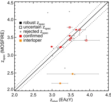
A condensed overview of the outcome of the automatic redshift search is provided in Fig.6. The results are listed in full detail in TableA.4, and illustrated for each galaxy in Figs. 7and8. In summary, we obtain a spectroscopic identification for 50% of our sample, with eight robust redshifts and four uncertain red-shifts, and find azphotcatastrophic failure rate of 8%, where the
contaminants arez∼2.5 dusty galaxies. We quantify the
accu-racy of the photometric redshifts to a median|z−zphot|of 1.2%,
which implies that even the galaxies withoutzspecshould be
re-liable. We describe these results in more detail in the following sub-sections.
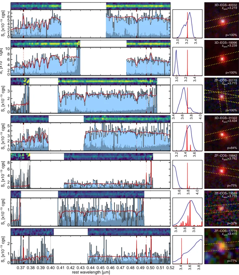
3.3.1. Robust redshifts
In total, we obtain eight robust spectroscopic identifications, withzspec ranging from 2.210 to 3.715. The highest measured
redshift,zspec=3.715, is that of ZF-COS-20115, which was first
reported inG17, and is based on the detection of Hβ, Hγ, and
Hδ absorption. We note that this value is slightly lower than
the redshift obtained in G17(zspec = 3.717); this results from
the accumulation of more data, and a slightly different
measure-ment method. The change, contained within the error bars, has no implication on the nature of the neighboring dusty source (Schreiber et al. 2018b). Balmer absorption lines are found in two other galaxies, 3D-EGS-18996 at zspec = 3.239 and
3D-EGS-40032 atzspec=3.219 (see Fig.7, top). These two galaxies
being at slightly lower redshifts, the rest of the Balmer series appears at the red end of the H band. Although at this stage
the continuum model was not yet fine-tuned to reproduce the strength of the Balmer absorption lines (this is done later in sec-tion4.1), the quality of the fit is already excellent. This illustrates the good agreement between the photometric and spectroscopic age-dating, which was already pointed out inG17and Schreiber et al. (2018b) when studying the case of ZF-COS-20115.
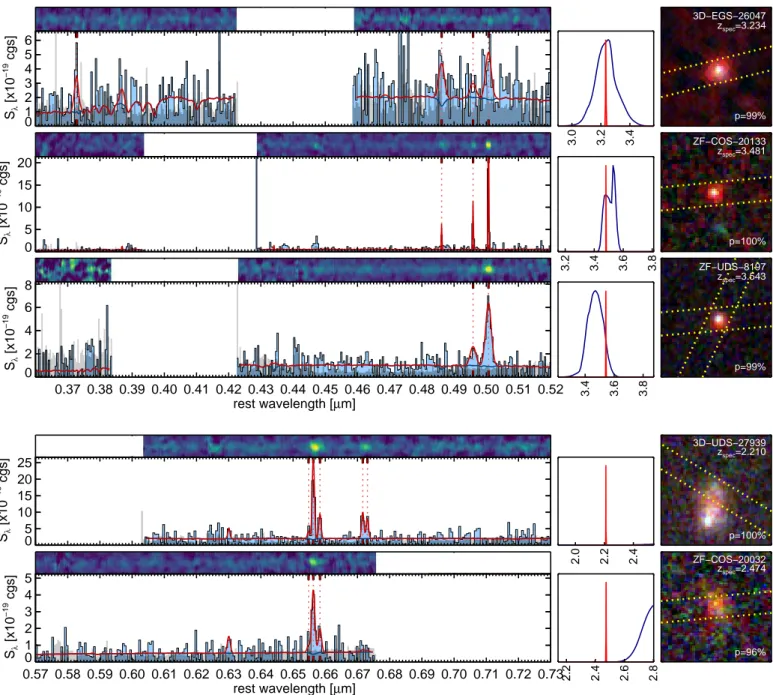
Beside these three galaxies, the rest of the redshifts were de-termined using emission lines. Two galaxies turn out to be red-shift interlopers, ZF-COS-20032 atzspec=2.474 and
3D-UDS-27939 atzspec = 2.210, for which we detected Hαand [Nii].
These two galaxies are shown in Fig.8(bottom). ZF-COS-20032 is significantly extended in the F160W image and is detected by ALMA at 890µm, which indicates it might be an obscured
disk. 3D-UDS-27939 is also extended, and blended with another galaxy. In the 3DHST catalog, this blended system was split in two galaxies, one of which was our target with zphot = 3.22,
while the other was attributed a lowerzphot =2.24±0.02. This
value is in fact consistent with our measuredzspec for the
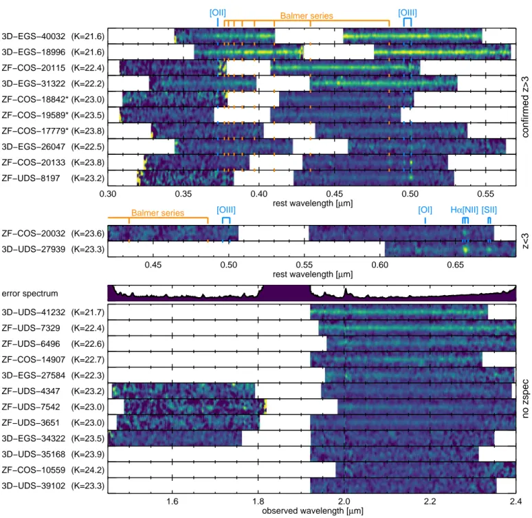
confirmed z>3
3D−EGS−40032 (K=21.6)
Balmer series
[OII] [OIII]
3D−EGS−18996 (K=21.6)
ZF−COS−20115 (K=22.4)
3D−EGS−31322 (K=22.2)
ZF−COS−18842* (K=23.0)
ZF−COS−19589* (K=23.5)
ZF−COS−17779* (K=23.8)
3D−EGS−26047 (K=22.5)
ZF−COS−20133 (K=23.8)
0.30 0.35 0.40 0.45 0.50 0.55
rest wavelength [µm]
ZF−UDS−8197 (K=23.2)
z<3
ZF−COS−20032 (K=23.6)
Balmer series [OIII] [OI] Hα[NII] [SII]
0.45 0.50 0.55 0.60 0.65
rest wavelength [µm] 3D−UDS−27939 (K=23.3)
no zspec
3D−UDS−41232 (K=21.7) error spectrum
ZF−UDS−7329 (K=22.4)
ZF−UDS−6496 (K=22.6)
ZF−COS−14907 (K=22.7)
3D−EGS−27584 (K=22.3)
ZF−UDS−4347 (K=23.2)
ZF−UDS−7542 (K=23.0)
ZF−UDS−3651 (K=23.0)
3D−EGS−34322 (K=23.5)
3D−UDS−35168 (K=23.9)
ZF−COS−10559 (K=24.2)
1.6 1.8 2.0 2.2 2.4
observed wavelength [µm] 3D−UDS−39102 (K=23.3)
Fig. 6: 2D spectra of our sample, flux-calibrated and corrected for telluric absorption. For display purposes only, these spectra were smoothed with a 70 Å boxcar filter in wavelength and 0.7′′ FWHM Gaussian along the slit. The galaxies are sorted by decreasing K-band continuumS/N.Top:Galaxies with a spectroscopic redshiftzspec>3, aligned on the same rest frame wavelength grid. The
most prominent emission and absorption lines are labeled in blue and orange ticks, respectively. Galaxies with an uncertain redshift (see text) are marked with an asterisk.Middle:Same as top but forzspec < 3.Bottom:Galaxies without spectroscopic redshift, aligned on the same observed wavelength grid. The average error spectrum is shown at the the top, to illustrate the regions with the strongest atmospheric features (telluric absorption and OH lines).
of the different mass-size relation for star-forming and quiescent
galaxies (e.g., van der Wel et al.2014a; Straatman et al.2015). The redshifts for the remaining three galaxies (ZF-COS-20133, 3D-EGS-26047, and ZF-UDS-8197) were obtained us-ing a combination of the [Oiii] doublet, Hβ, and [Oii].
ZF-COS-20133 and ZF-UDS-8197 are both found to have
partic-ularly bright [Oiii] emission and little to no Hβand [Oii], as
shown in Fig. 8. Their line widths, however, are very diff
er-ent: the former has unresolved line profiles (σv ≤ 60 km/s) in both [Oiii] and Hβ, while the latter has extremely broad [Oiii]