Contagious capital : a network analysis of interconnected intermediaries

(1)

Contagious Capital: A Network Analysis of Interconnected

Intermediaries

Jesse Blocher

A dissertation submitted to the faculty of the University of North Carolina at Chapel Hill in partial fulfillment of the requirements for the degree of Doctor of Philosophy in Business Administration (Finance) in the Department of Finance of the Kenan-Flagler Business School.

Chapel Hill 2012

Approved by:

Adam V. Reed, Advisor

Greg W. Brown

Jennifer Conrad

Joseph Engelberg

(2)

Abstract

JESSE BLOCHER: Contagious Capital: A Network Analysis of Interconnected Intermediaries.

(Under the direction of Adam V. Reed.)

I measure the effects of capital flow contagion in financial markets by analyzing portfolio

managers linked through interconnected asset holdings. My novel, network-based specification

provides estimates of shocks to common predictor variables 50-75% higher than existing

esti-mates of manager’s capital flows which ignore network relationships. This additional impact

arises because my network specification includes the effect of spillover onto immediate

neigh-bors and beyond, leading to feedback loops. My findings seem to result from crowded trades

(popular, short-term investment strategies) since network connections do not show strong

per-sistence and relatively small changes in asset allocation toward more concentrated positions

(3)

Acknowledgments

Thanks to my advisers for their patient and numerous reading of the poorly written early

drafts of this paper. Thanks to my wonderful wife for supporting me and my kids for being

excited to see me every day when I come home.

I am also grateful to Rick Sias (Discussant at the Financial Research Association

confer-ence), Chris Lundblad, Ed Van Wesep and Matt Ringgenberg for useful comments. Thanks

to Matthew Bothner (ESMT Management/Sociology) and Peter Mucha (UNC Mathematics)

for valuable guidance on network measures and computational algorithms, respectively. Ethan

Cohen-Cole and Tim Conley provided help and references on identification and econometrics.

James Moody and seminar participants at the Duke Network Analysis Center (dnac.ssri.

duke.edu) provided useful feedback, as did seminar participants at the SAMSI (www.samsi.

(4)

List of Tables

1 Fund Summary Statistics . . . 28

2 First Stage GMM Regression . . . 29

3 Effect of Peer Flows on Portfolio Returns . . . 31

4 Effect of Peer Flow on Fund Flows . . . 33

5 Contagion Effect of Peer Flows on Fund Flows - Long Run Steady State . . . . 34

6 Results removing sector funds – fund flows . . . 35

7 Results removing sector funds – portfolio returns . . . 37

8 Results removing the financial crisis – fund flows . . . 39

9 Results removing the financial crisis – portfolio returns . . . 41

(6)

List of Figures

1 Percentiles of portfolio distance measure through time. . . 24

2 The effect of a shock to cash holdings within a subset of portfolio managers. . . 25

3 The effect of a shock to portfolio returns within a subset of portfolio managers. 26

(7)

1. Introduction

Since the beginning of the recent financial crisis, the concept of

too-interconnected-to-fail has grown in importance, leading regulators to identify portfolio overlaps of financial

intermediaries as a potential source of systemic risk.1 Practitioners have also shown concern,

suggesting that “. . . there may be more crowded trades than most investors realize. If investors

exit at the same time, market movements could be chaotic.”2 Among academics, Stein (2009)

identifies “crowding”, or similar portfolios among sophisticated investors, as a risk in financial

markets and Brunnermeier and Sannikov (2011) identify portfolio overlaps as a destabilizing

mechanism in financial markets.

In this paper, I show that crowded trades may induce capital flow contagion among these

interconnected portfolio managers. Capital flow contagion occurs when the withdrawals and

forced sales experienced by one investment manager provoke capital outflows and asset sales

from other funds with similar portfolio holdings through the depressed prices of commonly

held assets (Brunnermeier and Pedersen (2009)).3 However, my approach accounts for broader

network propagation effects and feedback loops, not just pairwise connections. To do this, I

employ a novel instrumental variables specification to estimate contemporaneous capital flow

contagion effects in steady-state across the network.

Compared to the analysis of disconnected, independent portfolio managers common in

the literature, I find that coefficient estimates of common predictors of fund flows increase

1_{See speech by The Bank of England’s Executive Director for Financial Stability Andrew Haldane at}

http: //www.bankofengland.co.uk/publications/speeches/2010/speech433.pdf

2_Bank _of _{America-Merrill} _Lynch _report,

http://ftalphaville.ft.com/blog/2011/06/01/581676/ the-calm-before-the-volatility-storm/as quoted in the Financial Times, 1 June 2011.

3_{Brunnermeier and Pedersen (2009) model withdrawals and forced sales as a “market liquidity/funding}

(8)

by 50-75% when network relationships are taken into account.4 This increase is due to two

contagion processes I am able to incorporate with the full network of interconnections. First,

“own” effects increase by up to 20% due to feedback loops in which a shock to a manager

propagates out and back via a sequence of connected peers. Second, spillover effects (assumed

to be zero in non-network specifications) are substantial and increase estimates by an additional

30-55%. Spillover effects are similar to a network externality in which a shock to a manager

spills over onto his neighbors, such that an unsuspecting manager may find his portfolio under

stress due to funding problems by others holding a similar set of positions. Coval and Stafford

(2007) and Lou (2010) have established that fund flows impact asset prices. My innovation is

to consider the effect that these fund flows may have on the fund flows of neighbors holding

those same assets, since the same flow-performance relationship holds (Chevalier and Ellison

(1997)) even if asset prices change due to a peer’s forced sale.

I measure these effects with a network-based specification which includes connections

be-tween portfolio managers along with their capital flows at time t. This contemporaneous

specification allows me to estimate cross-sectional steady-state peer influence processes so the

effect of each portfolio manager on each other manager is estimated simultaneously. To identify

this influence process, I specify the two-step neighbor’s capital flow as an instrument. This is

a valid instrument if enough two-step neighbors are not themselves connected to the manager

of interest.5

I also show that the flows of connected neighbors are positively and significantly

corre-lated with a manager’s portfolio return; including these networked flow measures significantly

reduces the influence of market returns and fund category average flows as predictors. This

is a remarkable result since a portfolio manager’s own lagged fund flows show no significance

4_{Existing literature predicting fund flows assumes each fund to be independent (e.g. Sirri and Tufano}

(1998)). The common predictors of fund flows I consider are past returns, fund category average flows, and cash holdings.

5

(9)

in predicting returns (Frazzini and Lamont (2008)). It is also consistent with a contagion

process across managers connected by common holdings, since inflows would induce buying,

and outflows selling, of at least a portion of the commonly held portfolio.

To fully identify my network effect, I control for other possible explanations of correlated

flows. Specifically, since Sirri and Tufano (1998) show that the size of a mutual fund may

influence investor flows due to search costs, I control for both a manager’s own total net assets

and neighbor’s total net assets. In addition, since investor sector rotation strategies or other

strategic asset allocation decisions may induce flows to common categories, I include a category

average fund flow, similar to a Fama-French industry factor, as a control variable.

Given the result that capital flows seem to be contagious across similar portfolios, I next

address the nature of these portfolio connections. It may be that such connections are relatively

static, simply the result of natural linkages among varied strategies which are time invariant.

But it may also be that portfolio connections are transient and related to crowded trades, such

that interconnectedness may grow unobserved. To investigate these two hypotheses, I measure

the persistence of network connections through time. Static network connections should show

significant autoregressive properties, while transient crowded trades should show no long-term

temporal predictability among portfolio connections. I show that these connections among

portfolio managers are somewhat persistent short term, with network connections this quarter

correlating 0.4 with last quarter’s portfolio connections. However, the correlation across years

is approximately 0.13, with no correlation after two years. Since fund objectives are likely to

persist across several years, this suggests that shorter term connections are at least partially

driving my result.

To further investigate the nature of these portfolio connections, I demonstrate that the

similarity of two portfolios increases not only in terms of portfolio overlap, but also with

concentration in those commonly held assets. That is, two managers who overlap 20% of their

portfolio will be twice as connected if that overlap is in one holding than if it is equally held in

two holdings. The implication is that a mid-cap fund which holds hundreds of securities may

not connect other portfolios together as much as a fund with a few concentrated positions. It

(10)

connections to the extent that others hold similarly concentrated holdings. Small amounts of

overweighting compared to the manager’s benchmark may induce more interconnection than

a portfolio manager realizes.

First, I establish my hypotheses in the context of existing literature in Section 2. Next,

in Section 3, I describe my empirical approach to measuring capital flow contagion, detailing

network formation, measures, and methodology. In Section 4, I discuss my results, including

the interpretation of network coefficients and their economic significance. I then further analyze

the time-varying properties of my network and its relationship to crowded trades in Section 5,

after which I conclude with Section 6.

2. Hypotheses and Background

Quantifying the effects of capital flow contagion through interconnected asset holdings

implies hypotheses related to the prediction of mutual fund returns and mutual fund flows. I

first develop my hypothesis related to the prediction of portfolio returns which helps establish

portfolio overlaps as the mechanism for contagion. Second, I develop two hypotheses related

to the spillover effects of manager’s fund flows.

I propose that interconnected managers’ capital flows influence each other in the following

manner: inflows to neighboring portfolio managers induce purchases of their existing portfolio

and outflows induce sales, temporarily affecting the prices of those assets bought or sold.

But connected portfolio managers holding those same assets should see their portfolio returns

affected in a corresponding manner, such that the capital flows of connected portfolio managers

positively predict portfolio returns. Subsequently, since negative returns predict outflows and

positive returns predict inflows (Chevalier and Ellison (1997)), these affected managers may

experience their own inflows or outflows, perhaps beginning a market/funding liquidity spiral

(Brunnermeier and Pedersen (2009)). Thus, peer flows predict a portfolio manager’s returns

suggesting that interconnected portfolios are an important channel for capital flow contagion

in financial markets.

The fact that a portfolio manager’s fund flows affect the assets he holds is known. Coval

(11)

subsequent positive and negative returns, respectively. Lou (2010) addresses this question

across all fund flows, not just extreme positive and negative flows, and shows that this effect

is still significant but asymmetric – he estimates that one dollar of inflows correlates with

purchasing 0.6 dollars of the existing portfolio, while one dollar of outflows corresponds to

selling one dollar of the existing portfolio.

The “no arbitrage” condition in financial markets indicates that this mispricing should be

small or very short-term. But given that source of price pressure may be hidden (e.g., Kyle

(1985)), arbitrageurs may not identify a price movement as a deviation from fundamentals, and

thus not act to correct it. Arbitrageurs also face synchronization risk (Abreu and Brunnermeier

(2002, 2003)), since multiple arbitrageurs may be necessary to absorb the price pressure, as well

as other limits to arbitrage (e.g., Shleifer and Vishny (1997)). Indeed, rather than immediately

arbitraging an over- or under-pricing, these sophisticated investors may even exacerbate the

problem in a predatory manner to increase the mispricing and thus the profitability of a

subsequent convergence trade (Brunnermeier and Pedersen (2005)).

To identify common portfolio holdings as a channel of contagion, I hypothesize that the

fund flows of a manager’s connected neighbors predict portfolio returns through the buying

and selling of the commonly held assets. Formally,

Hypothesis 1: The fund flows of neighbors connected by common asset holdings positively

predict a manager’s portfolio return.

To test this hypothesis, I compute a measure of connected-neighbor fund flows weighted

by portfolio similarity, and then estimate its impact on portfolio returns. To determine my

baseline and control variables, I draw from the existing literature known predictor variables

of mutual fund returns. I include the market return which Carhart (1997) shows to be an

important predictor of mutual fund returns, as well as past flows to account for the

flow-performance relationship established in Chevalier and Ellison (1997). Since contemporaneous

fund flows and portfolio returns may suffer from endogeneity, I instrument peer flows in a

(12)

If connected-neighbor’s flows positively predict a manager’s portfolio returns, the next

log-ical step is to consider the effect on that manager’s fund flows, since returns affect future fund

flows. Chevalier and Ellison (1997) identify a performance-to-flow relationship such that

pos-itive past returns predict future inflows and poor past returns predict future outflows. While

Chevalier and Ellison measure these effects through lagged returns, these outflows could be

contemporaneous since a sophisticated manager, seeing his poor returns, may sell in

antici-pation of future outflows. Until now, investigating this relationship has been challenging due

to the endogeneity problem between contemporaneous flows and returns, a problem I solve

with my instrumental variables specification. This connection between the capital flows of

neighboring managers suggests two related hypotheses:

Hypothesis 2: The fund flows of neighbors connected by common asset holdings positively

predict a manager’s own fund flows.

Hypothesis 3: Spillover effects from each manager onto each other manager are nonzero.

While I could test Hypothesis 2 with lagged connected-neighbor fund flows in a simple

panel framework, that same specification would only provide indirect support for Hypothesis

3. To test both hypotheses, I employ a network specification which allows a

contemporane-ous equilibrium estimation of spillover effects across a network of connected agents. In this

network specification, I include other common predictors of capital flows such as past returns

(e.g.,Chevalier and Ellison (1997)), past flows (e.g., Coval and Stafford (2007)), total net

as-sets, and fund category average flows (e.g., Sirri and Tufano (1998)). I include my measure of

connected-neighbor fund flows as a predictor variable, instrumented by the two-step neighbor

fund flows. If the coefficient on this measure of peer’s capital flows is positive and significant,

this confirms Hypothesis 2: capital is contagious through interconnected portfolios.

While a positive and significant relationship establishes the existence of a contagion process,

obtaining evidence for Hypothesis 3 requires interpreting the resulting coefficient estimate.

Indeed, the richness of information available from this network specification constitutes a

(13)

an autoregression, but in the cross-section: fund flows at time t show up both as dependent

and independent variables, and as such the estimated coefficient on connected-neighbor flows

affects all other coefficient estimates in steady-state, similar to an temporal autoregression

framework.6 When the model is rearranged such that flows are only the dependent variable, the

coefficient on each independent variable becomes a matrix specifying the effect each portfolio

manager has on each other manager in equilibrium.7 This compares to the scalar coefficient

estimating the average effect in most other specifications. The average of the off-diagonals of

these matrix coefficients measures the spillover effects, while the average of the diagonal in

excess of the non-networked linear coefficient measures feedback effects. Nonzero off diagonals

in this matrix coefficient provides evidence of Hypothesis 3.

To test these hypotheses, I need to more fully specify the connection between portfolio

man-agers and how I measure the neighbor’s capital flows and estimate my network specification.

This is the topic of the next section.

3. Network Methodology

My network relationship derives from the connections among portfolio managers due to

common asset holdings but there are many concepts of interconnection in financial markets.

Allen, Babus, and Carletti (2010) and Zawadowski (2011) model connections among financial

intermediaries in the interbank market and Babus (2010) does the same for OTC markets.

Their analysis focuses on counterparty relationships in a game-theoretic framework in which

relationships are typically known and intentionally created by each market participant. My

measure of interconnection attempts to identify crowded trades in financial markets as a

sep-arate source of connectedness.

Others have studied the effect of common owners on financial assets. Kyle and Xiong

(2001) model convergence traders spanning disparate markets inducing comovement in the

assets they hold, and more recently Anton and Polk (2010) measure stock comovement as

6

Specifically, this model is a Spatial Auto-Regression (SAR), which is popular in spatial econometrics.

(14)

it relates to the number of common owners. Coval and Stafford (2007) and Jotikasthira,

Lundblad, and Ramadorai (2011) show that funding pressure on owners affects the assets they

hold, inducing price drops in those assets in U.S. and international settings, respectively. My

innovation is to consider what happens to other managers holding the same assets with no

funding pressure of their own, or spillover effects.

To describe my methodology in more detail, I describe my Data in Section 3.1. I then

de-velop my portfolio similarity measure in detail in Section 3.2 before proceeding to descriptions

of my GMM estimation approach, network instrument, and full specification in Section 3.3.

3.1. Data

My primary dataset is from Morningstar and contains the flows, returns, and full portfolio

holdings of U.S. Open Ended funds from 1998 to 2009.8 Flows of funds are a simple dollar value

per fund, per month or quarter. Note that my data includes reported values for both fund

flows and portfolio returns, whereas other studies typically compute fund flows from returns

and changes in total net assets. Because this data includes many bond funds and I want to

be as inclusive as possible, I keep any fund with nonzero equity position. I combine this data

with CRSP by CUSIP when necessary to obtain stock characteristics.

Importantly, this data contains the entire portfolio holdings of each open ended fund. This

means I have quarterly observations of each fund’s cash holdings as well rather than the less

frequent annual measures reported in the CRSP Mutual Fund database. In what follows,Flow

is always fund flow divided by total net assets as in Coval and Stafford (2007) andSize is the

log of total net assets. Cash is defined as currency, treasuries, and other cash-like holdings,

also divided by total net assets. I compute a fund-levelAmihud measure which is the portfolio

weighted sum of each equity holding’s individual Amihud measure over the previous quarter.

Summary statistics of these measures as well as peer measures are available in Table 1.

8

(15)

3.2. Portfolio Similarity Measure – The Network

My data represents a set of portfolio managers with detailed holdings data through time,

but for simplicity, I drop thetindex for this exposition and compute these measures for eacht.

I construct the similarity between two portfolios,sij as the dot product between the security

weight vectors of each portfolio manager i and j, divided by the product of the Euclidean

norm of each vector.9 _{Specifically,}

sij =

si·sj

|si| |sj|

(1)

where for each manager i, the Euclidean norm is defined across M securities as

|si|=

v u u t

M

X

m=1

s2_im (2)

Deriving this same measure in matrix form, let H be the holdings matrix, with portfolio

managers as each column, and each row consisting of the weight between 0 and 1 each manager

places on that security. My portfolio similarity measure is then

S = H

T_H

|H| · |H| (3)

in which each sij already defined above is an element of symmetric similarity matrix S. The

norm of the matrixH is a Euclidean column norm, such that for each columnj, the norm of

Hj is defined as

|Hj|=

v u u t

M

X

m=1

h2_jm (4)

Figure 1 plots percentiles of the distribution of this portfolio distance measure through time.

9

(16)

To construct Peer Flow for each manager i, I compute a weight vector which is each

similarity measuresij divided by the sum over all similarities, setting self-similaritysii to 0. I

then computePeer Flow as the dot product of the weight vector and the corresponding vector

of fund flows for each manager. Formally, peer weights are computed as

P eerW eightij =

sij

P

k

sik

, k6=i (5)

and Peer Flow is thus

P eerF lowi =

X

k

P eerW eightikF lowk (6)

For example, consider a portfolio manager with three neighbors at distances of 0.1, 0.2, and

0.1, such that the weights are.25,.50, and .25, respectively. If those neighbor’s flows (divided

by total net assets) are 0.01, 0.05, and 0.10, respectively, then Peer Flow is (.25∗.01) + (.5∗

.05) + (.25∗.10) = 0.0525.

In matrix form, if W is a row-stochastic transformation ofS, such that each row sums to

1, thenP eerF low =W ·F low in which bothPeerFlow and Flow areN×1 vectors andW is

anN×N matrix at timet. Note that I also compute other peer variables such as peer return,

peer size (total net assets), and peer cash (divided by total net assets) in the same way.10

3.3. Network Structure as Instrument

Since cross-sectional fund flows and returns of each portfolio manager at time t are

en-dogenous, I employ an instrument to identify influence rather than just correlation.11

With-out instrumentation, a correlation between two portfolio manager’s fund flows is not sufficient

evidence of one’s influence on the other.

Following Bramoull´e, Djebbari, and Fortin (2009), I employ a network-structure based

instrument to address this endogeneity based on “intransitive triads” which are often present

10_{This notion of portfolio distance is intuitively and mathematically similar to that of social distance as in}

Conley and Topa (2002).

11_{Since the diagonal of weighting matrix}_W _{is set to zero,}_{F lowi}_{is never on both sides of the same}

(17)

in a network. An intransitive triad is present if A connects to B and B to C, but A is not

connected to C. Thus, A can instrument for B’s influence on C since any influence A has on

C must be through the common relationship with B. In network terminology, A and C are

Two-Step neighbors, so my instrument isTwoStepPeerFlow.

For instance, a U.S. technology fund may be connected to a mid-cap fund through common

mid-cap technology holdings, and that mid-cap fund may also be connected to a Latin

Amer-ican fund through mid-cap Latin AmerAmer-ican holdings. Thus, the flows of the Latin AmerAmer-ican

fund can instrument for the mid-cap fund’s influence on the U.S. technology fund since they

are only connected through their common mid-cap neighbor.

However, not all two-step neighbors form intransitive triads. Additionally, while two

port-folio managers may not be directly connected, they both maintain some set relationship to

market-wide movements. Two-step neighbors can only serve as an instrument if they satisfy

the exclusion restriction – that the instrument is only correlated with the dependent variable

through the endogenous regressor. To address these concerns, Bramoull´e, Djebbari, and Fortin

(2009) specify a rank test which establishes that the instruments are not collinear with the

endogenous variable. To further test the validity of my instruments, I compute various tests

of weak instruments as well as Hansen’s J test of overidentification in all specifications. All

re-ported GMM specifications have results consistent with strong instruments and no correlation

of instruments with the second stage residual, thereby indicating a valid specification.

Mathematically, two-step neighbors are computed as B =S2, which is matrix

multiplica-tion (as opposed to element-by-element) where the diagonal of S has already been set to 0 to

avoid duplicating one-step and two-step neighbors.12 _{In summation notation, the equivalent}

product is

bij = N

X

q=1

siqsqj, q 6=i, j (7)

with the diagonal of B also set to zero such that a manager cannot be his own two-step

12_{A nonzero diagonal indicates a ‘self-loop.’ So, if}_S _{has a nonzero diagonal, a ‘two-step’ neighbor could be}

(18)

neighbor.13 If Wf is the row-stochastic, N ×N, two-step weighting matrix derived from B,

thenT woStepP eerF low=fW ·F low or as a summation

e wji =

bji

P

k

bjk

(8)

T woStepP eerF lowj =

X

k

e

wjkF lowk (9)

To ensure overidentification, I include not justT woStepP eerF low but also

T woStepP eerF low2 as excluded instruments, which is standard in an IV specification.

To test my first hypothesis, I instrument for peer fund flows as described above, but place

portfolio returns as my dependent variable. Specifically, I estimate:

P eerF lowit =T woStepP eerF lowit+T woStepP eerF low2it (10)

Retit =P eerF low\ it+F lowt−p+Rett−p

+Sizeit+Cashit+Amihudit+P eerSizeit

+P eerCashit+CategoryAvgF lowjt+M arketReturnt

(11)

with the primary explanatory variable beingM arketReturnin a CAPM style framework.14 If

P eerF lowis a positive predictor of portfolio returns, then it seems highly likely that commonly

held assets are the channel of influence.

Next, to test my second hypothesis that capital flows are contagious, I incorporate my

network measure in addition to common predictor variables in a specification with fund flows

as the dependent variable. Coval and Stafford (2007) employ both lagged flows and lagged

returns as predictors, and Sirri and Tufano (1998) show that fund category averages and fund

size (measured as log of total net assets) are important determinants of flows given investors’

non-zero search costs. Since temporary asset price movements may be stronger for illiquid

13

The diagonal ofBmust now be set to 0 because for every one-step neighbor, a manager is his own two-step neighbor. For instance,iconnects toj, but thenjalso connects back toi, such that for every connection like thisiis his own two-step neighbor.

14

(19)

securities, I include a portfolio-wideAmihud measure which is simply the weighted average of

the Amihud liquidity measure computed for each individual equity holding (Amihud (2002)).15

Since fund size is an important predictor of flows, I also include PeerSize as a control

variable. This control is important in a network specification because if flows primarily go

to larger funds (Sirri and Tufano (1998)), then funds who are both large and connected may

simply experience correlated flows without any mutual influence.

A portfolio manager’s cash holdings provide a vital cushion against unexpected

redemp-tions, and as such they likely influence the prediction of inflows and outflows. Most studies

exclude cash holdings because the data is unavailable, not because cash holdings are

unimpor-tant. Because I do have this data, I include it for both the manager and connected neightbors

(PeerCash), since a manager connected to cash-poor neighbors may be more susceptible to

flow contagion.

In sum, I estimate the following set of equations in a GMM specification:

P eerF lowit =T woStepP eerF lowit+T woStepP eerF low2it (12)

F lowit =P eerF low\ it+F lowt−p+Rett−p

+Sizeit+Cashit+Amihudit+P eerSizeit

+P eerCashit+CategoryAvgF lowjt

(13)

in which F undi ∈ Categoryj, 4 time lags are included (p = 4) and P eerF low\ it is the fitted

values from equations (12).16

15_{I also computed a full portfolio Amihud measure including cash and non-equity, non-cash holdings at the}

minimum and maximum Amihud measure, respectively, with similar results. Computed portfolio spreads and average daily volumes also gave similar results, available on request

16

Note that the exact specification of equation (12) includes all control variables in equation (13). To use strict GMM terminology,PeerFlow is the endogenous regressor, T woStepP eerF low andT woStepP eerF low2

(20)

3.4. Identification and Estimation of a Network Influence Process

In addition to the more standard identification problems already addressed, there are some

unique identification problems associated with network inference, which I now address following

the typology in Manski (1993). According to Manski (1993), identifying the endogenous social

influence process I have just described requires controlling for two other potential confounding

effects: “correlated effects” and “contextual effects.”17

“Correlated effects” simultaneously affect both connected managers due to common,

time-invariate characteristics. Correlated effects can be conceived as a cointegration relationship

where a relatively fixed relation among two neighbors induces a proportional response to

exogenous events. For example, two mutual funds, one half the size of the other, may find that

on average the smaller fund receives half the capital flows of the large one. Since there may

be a similar relationship due to cash holdings, I includePeerSize and PeerCash to control for

these potentially common fund characteristics which may drive correlated flows.

I control for Manski’s “contextual” effects by including CategoryAvgFlows, which

repre-sents the average flow for the Morningstar category to which each open ended fund belongs.

Contextual effects can be conceived as a network version of industry effects, in which

market-wide trends affect all members of the group equally, but may change across time. For instance,

a sector rotation strategy which suggests buying utilities and health care stocks in a declining

market represents a wider shift in investor behavior, operating above the level of individual

portfolio managers.

A further identification problem may arise due to network density, as noted by Kelejian,

Prucha, and Yuzefovich (2006). If I have a very dense or “complete” network such that everyone

is equally connected, each network member would have exactly the samePeerFlow measure.

For example, assume that each portfolio manager is connected to each other manager with a

weight of exactly 1. This would make PeerFlow equal to the average market-wide flow since

the weight on each flow variable would be _N1 for every manager and therefore no longer display

17_Bramoull´_{e, Djebbari, and Fortin (2009) also note that these controls are a necessary prerequisite for their}

(21)

cross-sectional variation. Given that my weighted density is less than 5%, this is unlikely to

be a problem. As a further robustness check, I have run my results thresholding my network

at the 80th percentile, thus obtaining an unweighted density of 10% with no material change

in results.18

Finally, I estimate this set of equations by Generalized Method of Moments, whereas most

specifications of this type in the spatial econometrics literature estimate this model via

Max-imum Likelihood. Conley (1999) notes that ML specifications in which spatial dependence is

measured with error are misspecified. While this is unlikely to be a problem with geographical

measures of distance typical of the spatial econometrics literature, my measure of distance in

security space may be much less precise. Fortunately, Kelejian and Prucha (2002) show that

with panel data, such as I have here, both OLS and GMM estimators are consistent, and thus

represents the appropriate estimation approach. Elhorst (2010) includes a short discussion on

ML vs IV/GMM estimators, noting that while the use of IV/GMM is promising, it is still new

to the spatial econometrics literature and needs further research.

4. Results

The baseline fund flow specification is from Sirri and Tufano (1998) and Coval and Stafford

(2007). They regress fund flow on lagged flows, lagged returns, fund size, and fund category

average flows at timet, with fund flow defined as dollar flows normalized by total net assets,

the same normalization I apply throughout. When I run this specification in a pooled OLS

and Fama-MacBeth framework, I get results qualitatively similar to Coval and Stafford (2007)

and others who have investigated this relationship such as Lou (2010) and Ferreira, Keswani,

Miguel, and Ramos (2011). However, I find it necessary to include both time and firm fixed

effects and further cluster my standard errors in both time and portfolio manager dimensions.

When I run both the Breusch-Pagan test and an F test on RSS of regressions with and

without time and firm fixed effects, I find that it is necessary to include some type of fixed or

18

Weighted density is the sum of all network connections in the network divided by the sum of all possible network connections set to 1, N2_{. Unweighted density is the same, but sets any weighted network link to 1}

(22)

random effects. A Hausman test verifies that fixed effects are necessary over random effects

(Kennedy (2008)). Clustering standard errors in both time and manager dimensions produces

large changes in standard errors indicating that this is a necessary step (Petersen (2009)).

I maintain this specification design throughout. Results from these tests as well as a table

comparing the varying differences in specification are available upon request.19 _{Including time}

fixed effects also controls for market wide events affecting all funds, and fund fixed effects

control for fund or fund manager time-invariant attributes.

4.1. Regression Results

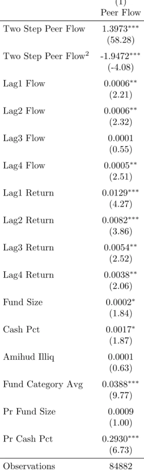
Our econometrics established, I turn to Table 2 which contains the results from the first

stage of the instrumental variables regression. The R2 of the Peer Flow regression is 0.83,

indicating the excellent fit necessary in a first stage regression.

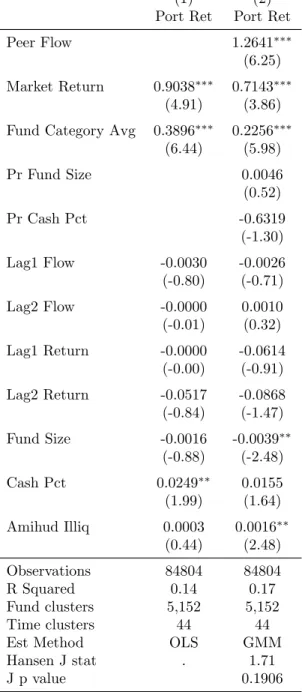
Next, I begin by regressingReturnon my networked and instrumentedP eerF lowvariable

as evidence that portfolio overlaps are driving a contagion effect, rather than a correlated flow

process. As shown in Table 3, there is a positive and significant coefficient onPeerFlow which

simultaneously increases the R2 from 0.14 to 0.17 and reduces the magnitude of both Market

Returnfrom 0.90 to 0.71 andCategory Avg Flowfrom 0.39 to 0.23, with all changes statistically

significant. That the fund flows from neighboring portfolio managers positively predict returns

is solid evidence that portfolio interconnections are the channel for this influence.

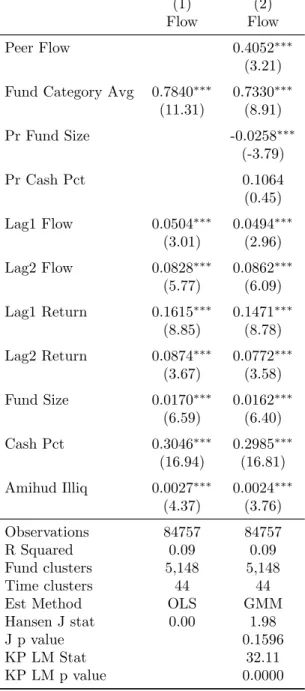
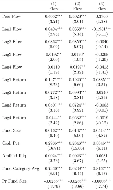
My main specification is in Table 4. Here,F lowis the dependent variable withP eerF low

as independent variable alongside other control variables. Again,P eerF lowenters in positively

and significantly with slight decreases in other predictor variables, indicating a flow contagion

process. However, sinceF lowenters into the specification both as dependent and independent

variable, I must transform the equation similar to an autoregression specification to fully

interpret this coefficient.

19

(23)

4.2. Network Coefficient Interpretation

To interpret the coefficient on Model 2 in Table 4, I begin by rewriting my specification in

Equation 13 in matrix form, without the instrumentation:20

Ft=ρsWtFt+ρtFt−1+Xtβ+ (14)

in which Ft is theN×1 vector of fund flows at timet. Wtis a row-stochastic transformation

ofN×N portfolio similarity matrixSat timet, such thatP eerF lowt=Wt·Ft. Xtrepresents

all other control and explanatory variables for simplicity.

Next, I group together all terms involving Ft, also setting Ft = Ft−1 to incorporate a

steady-state process.21 Since flows are not persistent, this is a trivial simplification. The

result is

((1−ρt)IN −ρsWt)Ft=Xtβ+ (15)

Ft=X1tβ˜1+X2tβ˜2+. . .+XP tβ˜P + (16)

for each p= 1. . . P explanatory variables. Each actual estimated coefficient is

˜

βp,N×N = ((1−ρt)IN−ρsWt)−1βp (17)

which is an N ×N matrix. Without my network specification, the comparable coefficient

would be the scalar coefficient estimate times anN ×N identity matrix.

In equation 17, βReturn is the sum of the return coefficients from Model 2 in Table 4 since

in steady-state,t=t−p∀p. Since P eerCash=W ·Cash,βCash is the sum of the coefficient

onCash times the identity matrix plus the coefficient onPeerCash timesW. Mathematically,

20

For this analysis, I simply use the endogenous PeerFlow rather than the predicted value from the first stage regression, which simplifies the exposition and likely is a good approximation since the R2 _{of the first}

stage regression is 0.83. However, I still use the coefficient estimates from the instrumented specification.

21_{Note that in my specification, I have 4 Flow lags, so}_Ft₌_Ft

(24)

if βC is the regression coefficient on Cash and βP C is the regression coefficient on PeerCash,

then the overall effect of cash, βCash is

βCash=βC ·I+βP C·W (18)

βCategoryAvgF low is simply the corresponding estimated coefficient from Model 2 in Table 4.

To interpret this network coefficient, I divide it into feedback effects, represented by the

diagonal, and spillover effects which reside on the off-diagonal. The results for important

explanatory variables are in Table 5. The first column is the scalar coefficient estimate, β,

without the network transformation. Next are the incremental feedback effects, computed as

the average of the diagonal less the scalar coefficient. Finally, spillover effects are computed

as the average of all off-diagonal entries in the network coefficient.

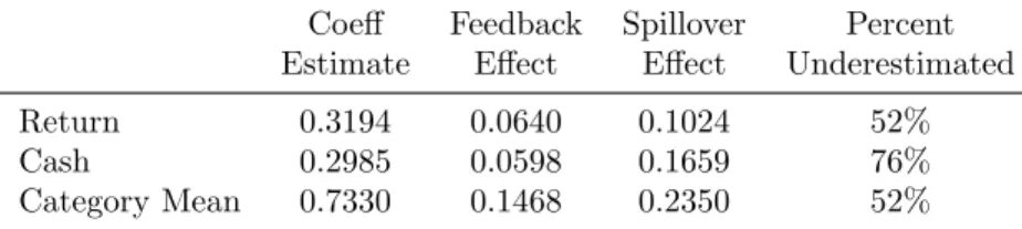
Table 5 shows how my network specification accounts for feedback and spillover effects,

increasing estimate by up to 76%. Specifically, returns and category average flows show effects

that are 52% greater than non-networked effects, and networked cash holdings effects are 76%

greater.

To illustrate spillover, I simulate a shock to approximately 40% of the fund managers in

the sample and measure the impact to the other 60%, which is assumed to be zero in a

non-networked specification. I shock Cash by one standard deviation, simulating an unexpected

redemption, and I shockReturns by one standard deviation, simulating an unexpected market

movement.22 The results are illustrated in Figure 2 and Figure 3. Note that these spillover

effects are as large as 0.01, which is the mean value of flow and approximately 10% of the

standard deviation, available in Table 1.

To more fully identify capital flow contagion as a unique phenomena, I perform several

ro-bustness checks. I re-run my main specification removing all sector funds from the dataset, and

22_{Since managers are connected by assets, for this to be an isolated shock, it could be to non-equity holdings}

(25)

find the result strengthened – the coefficient is larger and estimated with more precision.23,24

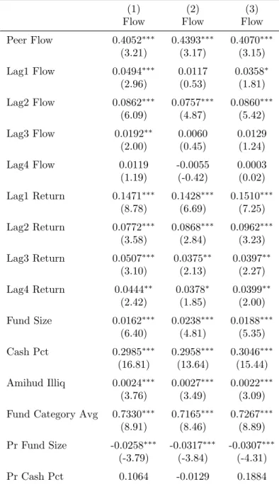
Results with and without sector funds are presented in Tables 6 and 7. In Table 6, the

contagion process in Model 2 without sector funds is almost 25% greater than the baseline

including them (0.50 compared to 0.41) whereas sector funds alone show no significance. Fund

Category Avg is also smaller without sector funds, at 0.62 vs 0.73 in the baseline result. Among

sector funds only, this same control is 0.82, indicating that Fund Category Avg is a primary

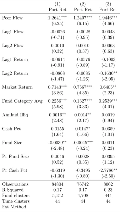
driver of sector fund flows. In Table 7, there is very little difference between the models with

and without sector funds, displayed in Models 1 and 2. Fund Category Avg drops from 0.23 to

0.13, indicating that whileP eerF lowand Fund Category Avgoverlap somewhat among sector

funds, they are much less related in the broader sample.

Since financial crises induce correlations across disparate asset groups, it is possible that my

result is simply arising from the recent financial crisis. Accrodingly, I re-run my specification

omitting the financial crisis, stopping my analysis in the second quarter of 2007 and 2008,

respectively, with results presented in Tables 8 and 9. Interestingly, the flow contagion effect

is stronger when omitting the financial crisis. This can be seen in Model 2 of Table 8, in which

the P eerF low coefficient rises moderately (though without statistical significance) from 0.41

to 0.44. Table 9 presents the results for returns, again showing no marked difference.

5. Crowded Trades and Network Persistence

Having provided evidence that portfolio interconnections may induce capital flow contagion,

I proceed to investigate the nature of these connections. If these portfolio connections are

relatively persistent, then this static set of connections may be more easily identified from

public holdings disclosures by both market participants and regulators alike. On the other

hand more transient portfolio interconnections may make capital flow contagion effects much

23

Sector funds are those labeled Technology, Utilities, Financials, etc. corresponding to equities held in a specific industry.

24_{Note that this is a simple division of my sample which only considers the portfolio managers who are}

(26)

harder to detect ex ante.

Between the two, transient or hard-to-observe portfolio interconnections pose the greater

risk to portfolio managers and regulators alike since a hidden contagion process is more likely

to generate unexpected negative shocks. These transient portfolio interconnections may arise

due to so-called “crowded trades”, which occur when portfolio managers take concentrated or

overweighed positions in a small set of stocks.25 Due to lags in mandatory disclosures, crowded

trades may not be detectable to market participants until many months after the trades are

established. Thus, with no knowledge of network connections, negative flow shocks across

portfolio connections will be unanticipated and likely produce greater negative consequences

than shocks which are at least partially anticipated.

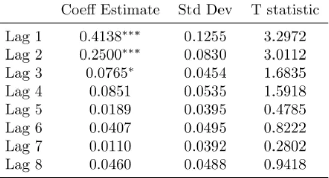
Table 10 presents the results of an autoregression on my network measure, similar to the

main specification in Anton and Polk (2010). This specification takes the N ×N network of

relationships between all of the portfolio managers at time tand puts them in aN×1 vector

as the dependent variable. Then the same network of relationships at t−1, t−2, enter as

independent variables, vectorized. I then run this regression for each time t and summarize

the coefficients across time in a Fama-MacBeth framework.

The marginal effects of the lags diminish to be statistically insignificant after 3 lags, but

still show some autoregressive properties. The network distance correlation lagged one quarter

is 0.41, which indicates some short-term persistence. To estimate the correlation two quarters

previous, I compute 0.412+ 0.25 = 0.42, showing that the persistence extends to the previous

six months. But the correlation between the network distance measure and that 3 quarters past

is 0.413_{+ 0.25}2_{+ 0.765 = 0.21, a significant drop off, and then one year past is 0.41}4_{+ 0.25}3₊

0.082+ 0.0 = 0.05 if I treat the insignificant 4th lag as 0, or 0.13 if I retain it. After two years,

retaining the first four coefficients, the correlation is 0.418+ 0.257+ 0.086 + 0.085 = 0.0009,

which is very close to 0.26 Since portfolio objectives likely persist greater than two years,

25

Crowded trades are also related to the herding literature. Sias (2004) summarizes the broad classifications motivating herding. Rationally, managers herd on correlated private information (Froot, Scharfstein, and Stein (1992)). Other explanations include reputation-based herding (Scharfstein and Stein (1990)), and fads (Barberis and Shleifer (2003)).

26

(27)

this suggests that there is some transience to my measure of interconnectedness and thus that

crowded trades or herding among institutional managers plays a role in capital flow contagion.

Finally, to further investigate the nature of portfolio connectivity, I show that my

nor-malized dot product distance measure increases in two dimensions. First, it is increasing in

portfolio overlap, which is its primary purpose. As the percentage of portfolio overlap

in-creases, the distance between two managers in security space decreases (they are more similar

in security space). But, perhaps less intuitively, my portfolio distance measure is also

in-creasing in the concentration of those holdings. This is illustrated in Figure 4. Holding total

portfolio overlap constant, a single concentrated position gives twice as much similarity as two

overlapping holdings of equal proportion. This property of my portfolio distance measure

indi-cates that concentrated positions give rise to more interconnectedness. Accordingly, crowding

or overweighting in a specific set of securities may induce more connectedness among those

managers than they may realize.

6. Conclusion

In the wake of the recent financial crisis, the interconnection of market participants has

become an important new area of research. Employing a novel, network-based specification,

I show that interconnected intermediaries exhibit contagious capital flows, exposing them

to feedback effects and spillover effects which result in estimates 50-75% greater than

non-networked coefficients. To incorporate these network connections simultaneously, I

contem-poraneously estimate the influence of each portfolio manager’s capital flows on each other

manager by exploiting the network structure as an instrument.

I also have shown some evidence that that these contagious flows are the result of crowded

trades – short-term, popular market positions – since portfolio connection exhibits only a

small amount of short-term persistence. Furthermore, I have illustrated how distances between

portfolios in security space emphasize concentrated positions, such that active managers

over-weighting portions of their portfolio may unintentionally increase their dependence on similar

(28)

While my analysis focuses on the equity holdings of open ended funds, it also has

implica-tions for collateralized financing. Financial intermediaries who rely on collateralized

(whole-sale) financing to fund their investments are growing in market share (Adrian and Shin (2010)).

It may be that my results imply a broader “collateral contagion” effect which could have played

a role in recent runs on repo financing (Gorton and Metrick (2011)). Since even interbank

lending is becoming more collateralized, Allen and Gale (2000)’s canonical model of interbank

financial contagion may be further amplified by connected collateral.27

This work also provides motivation for the collection of more detailed holdings data from

market participants, since the results described herein can be characterized as a negative

network externality which may merit government regulation. Indeed, Brunnermeier, Hansen,

Kashyap, Krishnamurthy, and Lo (2011) recently responded to an AEA/NSF call for proposals

on “grand challenge questions” for research in the next ten years by advocating the collection

of additional data and developing network models in the pursuit of quantifying systemic

finan-cial risk. While immediate public disclosure may have unintended predatory trading effects

(Brunnermeier and Pedersen (2005)), confidential disclosure to regulatory bodies and/or

de-layed public disclosure are likely to be beneficial and could be the purview of the newly formed

Office of Financial Research established by the Dodd-Frank Act.

While network methods are becoming more popular in corporate finance (e.g., Hochberg,

Ljungqvist, and Lu (2007); Cohen, Frazzini, and Malloy (2008); Ahern and Harford (2010)) and

market microstructure (Cohen-Cole, Kirilenko, and Patacchini (2010)), little has been done

applying network methods to equity markets. My network approach allows a steady-state

analysis of this peer influence process in the cross-section, bringing structure to cross-sectional

analysis previously only available in the time series. While I have applied it to portfolio

interconnections, it may also have broad applicability to other areas such as interbank lending

(e.g. Cohen-Cole, Patacchini, and Zenou (2011)) or stock market volatility (Greenwood and

Thesmar (2011)). And in a time when bailouts are motivated not because of too-big-to-fail,

27

(29)

but because of too-interconnected-to-fail, understanding and quantifying the interconnections

(30)

(31)

(32)

(33)

(34)

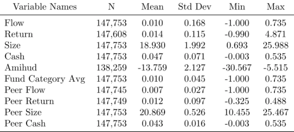
Table 1: Fund Summary Statistics

Summary statistics for fund data as used in regression specifications. Flow is dollar flows divided by total net assets and Cash is cash holdings divided by total net assets. Size is log of total net assets. Amihud is a portfolio weighted measure of the Amihud values of equity holdings, logged. Fund Category Average is the average Flow across Morningstar categories. Peer variables are weighted by network connections. Data is quarterly from 1995 to 2009.

Variable Names N Mean Std Dev Min Max

(35)

Table 2: First Stage GMM Regression

First stage regressions with endogenous regressors as dependent variables. Peer Flow is the weighted average of peer connected flow, and Two Step Peer Flow is the same of their neighbor’s neighbors, used as instruments. Flow is dollar flows divided by total net assets and Cash is cash holdings divided by total net assets. Size is log of total net assets. Amihud is a portfolio weighted measure of the Amihud values of equity holdings, logged. Fund Category Average is the average Flow across Morningstar categories. Data is quarterly from 1995 to 2009. Time and Fund Fixed Effects included. T statistics are in parentheses and significance is denoted at the 1, 5, and 10% level.

(1) Peer Flow

Two Step Peer Flow 1.3973∗∗∗ (58.28)

Two Step Peer Flow2 _-1.9472∗∗∗

(-4.08)

Lag1 Flow 0.0006∗∗ (2.21)

Lag2 Flow 0.0006∗∗ (2.32)

Lag3 Flow 0.0001 (0.55)

Lag4 Flow 0.0005∗∗ (2.51)

Lag1 Return 0.0129∗∗∗ (4.27)

Lag2 Return 0.0082∗∗∗ (3.86)

Lag3 Return 0.0054∗∗ (2.52)

Lag4 Return 0.0038∗∗ (2.06)

Fund Size 0.0002∗ (1.84)

Cash Pct 0.0017∗ (1.87)

Amihud Illiq 0.0001 (0.63)

Fund Category Avg 0.0388∗∗∗ (9.77)

Pr Fund Size 0.0009 (1.00)

Pr Cash Pct 0.2930∗∗∗

(6.73)

Observations 84882

(36)

(1) Peer Flow

(37)

Table 3: Effect of Peer Flows on Portfolio Returns

Portfolio return is the dependent variable, provided by Morningstar. Data is quarterly from 1998 to 2009, each panel variable is any open ended fund holding a nonzero equity position. Network relation is the normalized dot product, and peer effects are the weighted average of peer characteristics. Flow is the fund flow divided by total net assets. Fund size is the log of total net assets. Cash Pct is cash holdings divided by total net assets. Amihud is the portfolio weighted sum of equity holdings’ Amihud measures computed over the previous quarter. Market return is CRSP value weighted market return, and Category Avg Flow is the average of all reported fund flows by Morningstar category. Flow and return lags 3 and 4 included but not shown. Time and Fund Fixed Effects included. Hansen J stat is a test of overidentification for which the null hypothesis is that instruments are uncorrelated with stage 2 regression, KP LM stat tests the null of weak instruments. T statistics are in parentheses and significance is denoted at the 1, 5, and 10% level.

(1) (2) Port Ret Port Ret

Peer Flow 1.2641∗∗∗ (6.25)

Market Return 0.9038∗∗∗ 0.7143∗∗∗ (4.91) (3.86)

Fund Category Avg 0.3896∗∗∗ 0.2256∗∗∗ (6.44) (5.98)

Pr Fund Size 0.0046 (0.52)

Pr Cash Pct -0.6319 (-1.30)

Lag1 Flow -0.0030 -0.0026 (-0.80) (-0.71)

Lag2 Flow -0.0000 0.0010 (-0.01) (0.32)

Lag1 Return -0.0000 -0.0614 (-0.00) (-0.91)

Lag2 Return -0.0517 -0.0868 (-0.84) (-1.47)

Fund Size -0.0016 -0.0039∗∗ (-0.88) (-2.48)

Cash Pct 0.0249∗∗ 0.0155 (1.99) (1.64)

Amihud Illiq 0.0003 0.0016∗∗ (0.44) (2.48)

Observations 84804 84804 R Squared 0.14 0.17 Fund clusters 5,152 5,152 Time clusters 44 44 Est Method OLS GMM Hansen J stat . 1.71 J p value 0.1906

(38)

(1) (2) Port Ret Port Ret

(39)

Table 4: Effect of Peer Flow on Fund Flows

Flow ratio is the dependent variable and is the fund flow divided by total net assets. Data is quarterly from 1998 to 2009, each panel variable is any open ended fund holding a nonzero equity position. Network relation is the normalized dot product, and peer effects are the weighted average of peer characteristics. Fund size is the log of total net assets. Cash Pct is cash holdings divided by total net assets. Amihud is the portfolio weighted sum of equity holdings’ Amihud measures computed over the previous quarter. Category Avg Flow is the average of all reported fund flows by Morningstar category. Flow and return lags 3 and 4 included but not shown. Time and Fund Fixed Effects included. Hansen J stat is a test of overidentification for which the null hypothesis is that instruments are uncorrelated with stage 2 regression, KP LM stat tests the null of weak instruments. T statistics are in parentheses and significance is denoted at the 1, 5, and 10% level.

(1) (2) Flow Flow

Peer Flow 0.4052∗∗∗ (3.21)

Fund Category Avg 0.7840∗∗∗ 0.7330∗∗∗ (11.31) (8.91)

Pr Fund Size -0.0258∗∗∗ (-3.79)

Pr Cash Pct 0.1064 (0.45)

Lag1 Flow 0.0504∗∗∗ 0.0494∗∗∗ (3.01) (2.96)

Lag2 Flow 0.0828∗∗∗ 0.0862∗∗∗ (5.77) (6.09)

Lag1 Return 0.1615∗∗∗ 0.1471∗∗∗ (8.85) (8.78)

Lag2 Return 0.0874∗∗∗ 0.0772∗∗∗ (3.67) (3.58)

Fund Size 0.0170∗∗∗ 0.0162∗∗∗ (6.59) (6.40)

Cash Pct 0.3046∗∗∗ 0.2985∗∗∗ (16.94) (16.81)

Amihud Illiq 0.0027∗∗∗ 0.0024∗∗∗ (4.37) (3.76)

(40)

Table 5: Contagion Effect of Peer Flows on Fund Flows - Long Run Steady State

Contagion effect based on Model 2 in Table 4, assuming long run and cross-sectional equilibrium (through time and across funds). Coeff Estimate is non-networked estimate, Feedback Effect includes the incremental average spillover effects which circulate back to the same fund, Spillover effect is the average off-diagonal effects among portfolio managers. Data is quarterly from 1998 to 2009, each panel variable is any open ended fund holding a nonzero equity position. Network relation is the normalized dot product. Category Avg Flow is the average of all reported fund flows by Morningstar category.

Coeff Feedback Spillover Percent Estimate Effect Effect Underestimated

(41)

Table 6: Results removing sector funds – fund flows

Fund flow divided by total net assets is the dependent variable, provided by Morningstar. Model 1 is the baseline, taken from Model 2 of Table 4. Model 2 is the same, but with sector funds omitted from the analysis. Model 3 includes only sector funds. Sector funds are mutual funds with an industry-specific category, such as Technology or Health Care. Data is quarterly from 1998 to 2009, each panel variable is any open ended fund holding a nonzero equity position. Network relation is the normalized dot product, and peer effects are the weighted average of peer characteristics. Fund size is the log of total net assets. Cash Pct is cash holdings divided by total net assets. Amihud is the portfolio weighted sum of equity holdings’ Amihud measures computed over the previous quarter. Market return is CRSP value weighted market return, and Category Avg Flow is the average of all reported fund flows by Morningstar category. Time and Fund Fixed Effects included. Hansen J stat is a test of overidentification for which the null hypothesis is that instruments are uncorrelated with stage 2 regression, KP LM stat tests the null of weak instruments. T statistics are in parentheses and significance is denoted at the 1, 5, and 10% level.

(1) (2) (3) Flow Flow Flow

Peer Flow 0.4052∗∗∗ 0.5028∗∗∗ 0.3706 (3.21) (3.61) (1.38)

Lag1 Flow 0.0494∗∗∗ _0.0868∗∗∗ _-0.1951∗∗∗

(2.96) (5.14) (-5.11)

Lag2 Flow 0.0862∗∗∗ _0.0859∗∗∗ _-0.0040

(6.09) (5.97) (-0.14)

Lag3 Flow 0.0192∗∗ 0.0193∗ -0.0268 (2.00) (1.95) (-1.20)

Lag4 Flow 0.0119 0.0197∗∗ -0.0413 (1.19) (2.12) (-1.41)

Lag1 Return 0.1471∗∗∗ 0.1920∗∗∗ 0.0885∗∗∗ (8.78) (9.60) (3.51)

Lag2 Return 0.0772∗∗∗ 0.0993∗∗∗ 0.0240 (3.58) (3.81) (1.35)

Lag3 Return 0.0507∗∗∗ 0.0724∗∗∗ -0.0003 (3.10) (3.92) (-0.01)

Lag4 Return 0.0444∗∗ 0.0632∗∗∗ -0.0019 (2.42) (2.86) (-0.12)

Fund Size 0.0162∗∗∗ 0.0137∗∗∗ 0.0514∗∗∗ (6.40) (5.90) (4.82)

Cash Pct 0.2985∗∗∗ 0.2846∗∗∗ 0.3845∗∗∗ (16.81) (15.06) (6.14)

Amihud Illiq 0.0024∗∗∗ 0.0023∗∗∗ 0.0031 (3.76) (3.67) (1.25)

Fund Category Avg 0.7330∗∗∗ 0.6238∗∗∗ 0.8167∗∗∗ (8.91) (6.44) (6.17)

Pr Fund Size -0.0258∗∗∗ -0.0256∗∗∗ -0.0608∗∗∗ (-3.79) (-3.66) (-2.74)

(42)

Pr Cash Pct 0.1064 0.0981 -0.1813 (0.45) (0.40) (-0.38)

Observations 84757 76698 8059 R Squared 0.09 0.09 0.18 Fund clusters 5,148 4,704 444 Time clusters 44 44 44 Est Method

(43)

Table 7: Results removing sector funds – portfolio returns

Portfolio return is the dependent variable, provided by Morningstar. Model 1 is the baseline, taken from Model 2 of Table 3. Model 2 is the same, but with sector funds omitted from the analysis. Model 3 includes only sector funds. Sector funds are mutual funds with an industry-specific category, such as Technology or Health Care. Data is quarterly from 1998 to 2009, each panel variable is any open ended fund holding a nonzero equity position. Network relation is the normalized dot product, and peer effects are the weighted average of peer characteristics. Fund size is the log of total net assets. Cash Pct is cash holdings divided by total net assets. Amihud is the portfolio weighted sum of equity holdings’ Amihud measures computed over the previous quarter. Market return is CRSP value weighted market return, and Category Avg Flow is the average of all reported fund flows by Morningstar category. Time and Fund Fixed Effects included. Hansen J stat is a test of overidentification for which the null hypothesis is that instruments are uncorrelated with stage 2 regression, KP LM stat tests the null of weak instruments. T statistics are in parentheses and significance is denoted at the 1, 5, and 10% level.

(1) (2) (3) Port Ret Port Ret Port Ret

Peer Flow 1.2641∗∗∗ 1.2407∗∗∗ 1.9446∗∗∗ (6.25) (6.15) (4.66)

Lag1 Flow -0.0026 -0.0028 0.0043 (-0.71) (-0.95) (0.39)

Lag2 Flow 0.0010 0.0010 0.0063 (0.32) (0.37) (0.63)

Lag1 Return -0.0614 -0.0576 -0.1003 (-0.91) (-0.89) (-1.17)

Lag2 Return -0.0868 -0.0685 -0.1630∗∗ (-1.47) (-1.26) (-2.05)

Market Return 0.7143∗∗∗ 0.7567∗∗∗ 0.6405∗∗ (3.86) (4.35) (2.23)

Amihud Illiq 0.0016∗∗ 0.0014∗∗ 0.0019 (2.48) (2.17) (0.94)

Cash Pct 0.0155 0.0147∗ 0.0359 (1.64) (1.66) (1.01)

Fund Size -0.0039∗∗ -0.0045∗∗∗ 0.0011 (-2.48) (-3.24) (0.23)

Pr Fund Size 0.0046 0.0028 0.0395 (0.52) (0.35) (1.12)

Pr Cash Pct -0.6319 -0.3495 -2.7786∗∗ (-1.30) (-0.80) (-2.50)

Observations 84804 76742 8062 R Squared 0.17 0.17 0.23 Fund clusters 5,152 4,708 444 Time clusters 44 44 44 Est Method

(44)

(45)

Table 8: Results removing the financial crisis – fund flows

Fund flow divided by total net assets is the dependent variable, provided by Morningstar. Model 1 is the baseline, taken from Model 2 of Table 4, ranging from 1998 to 2009. Model 2 is the same, but only including quarters from 1998 through the second quarter of 2007. Model 3 extends through the second quarter of 2008. Each panel variable is any open ended fund holding a nonzero equity position. Network relation is the normalized dot product, and peer effects are the weighted average of peer characteristics. Fund size is the log of total net assets. Cash Pct is cash holdings divided by total net assets. Amihud is the portfolio weighted sum of equity holdings’ Amihud measures computed over the previous quarter. Market return is CRSP value weighted market return, and Category Avg Flow is the average of all reported fund flows by Morningstar category. Time and Fund Fixed Effects included. Hansen J stat is a test of overidentification for which the null hypothesis is that instruments are uncorrelated with stage 2 regression, KP LM stat tests the null of weak instruments. T statistics are in parentheses and significance is denoted at the 1, 5, and 10% level.

Peer Flow 0.4052∗∗∗ _0.4393∗∗∗ _0.4070∗∗∗

(3.21) (3.17) (3.15)

Lag1 Flow 0.0494∗∗∗ _0.0117 _0.0358∗

(2.96) (0.53) (1.81)

Lag2 Flow 0.0862∗∗∗ 0.0757∗∗∗ 0.0860∗∗∗ (6.09) (4.87) (5.42)

Lag3 Flow 0.0192∗∗ 0.0060 0.0129 (2.00) (0.45) (1.24)

Lag4 Flow 0.0119 -0.0055 0.0003 (1.19) (-0.42) (0.02)

Lag1 Return 0.1471∗∗∗ 0.1428∗∗∗ 0.1510∗∗∗ (8.78) (6.69) (7.25)

Lag2 Return 0.0772∗∗∗ 0.0868∗∗∗ 0.0962∗∗∗ (3.58) (2.84) (3.23)

Lag3 Return 0.0507∗∗∗ 0.0375∗∗ 0.0397∗∗ (3.10) (2.13) (2.27)

Lag4 Return 0.0444∗∗ 0.0378∗ 0.0399∗∗ (2.42) (1.85) (2.00)

Fund Size 0.0162∗∗∗ 0.0238∗∗∗ 0.0188∗∗∗ (6.40) (4.81) (5.35)

Cash Pct 0.2985∗∗∗ 0.2958∗∗∗ 0.3046∗∗∗ (16.81) (13.64) (15.44)

Amihud Illiq 0.0024∗∗∗ 0.0027∗∗∗ 0.0022∗∗∗ (3.76) (3.49) (3.09)

Pr Fund Size -0.0258∗∗∗ -0.0317∗∗∗ -0.0307∗∗∗ (-3.79) (-3.84) (-4.31)

Pr Cash Pct 0.1064 -0.0129 0.1884

(46)

(0.45) (-0.06) (0.77)

Observations 84757 59376 70554 R Squared 0.09 0.09 0.09 Fund clusters 5,148 4,485 4,839 Time clusters 44 35 39 Est Method

(47)

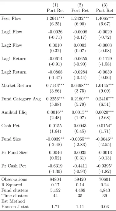
Table 9: Results removing the financial crisis – portfolio returns

Portfolio return is the dependent variable, provided by Morningstar. Model 1 is the baseline, taken from Model 2 of Table 3, ranging from 1998 to 2009. Model 2 is the same, but only including quarters from 1998 through the second quarter of 2007. Model 3 extends through the second quarter of 2008. Each panel variable is any open ended fund holding a nonzero equity position. Network relation is the normalized dot product, and peer effects are the weighted average of peer characteristics. Fund size is the log of total net assets. Cash Pct is cash holdings divided by total net assets. Amihud is the portfolio weighted sum of equity holdings’ Amihud measures computed over the previous quarter. Market return is CRSP value weighted market return, and Category Avg Flow is the average of all reported fund flows by Morningstar category. Time and Fund Fixed Effects included. Hansen J stat is a test of overidentification for which the null hypothesis is that instruments are uncorrelated with stage 2 regression, KP LM stat tests the null of weak instruments. T statistics are in parentheses and significance is denoted at the 1, 5, and 10% level.

Peer Flow 1.2641∗∗∗ _1.2432∗∗∗ _1.4065∗∗∗

(6.25) (6.90) (6.67)

Lag1 Flow -0.0026 -0.0008 -0.0029 (-0.71) (-0.17) (-0.72)

Lag2 Flow 0.0010 0.0003 -0.0003 (0.32) (0.07) (-0.08)

Lag1 Return -0.0614 -0.0655 -0.1129 (-0.91) (-0.90) (-1.58)

Lag2 Return -0.0868 -0.0284 -0.0039 (-1.47) (-0.44) (-0.06)

Market Return 0.7143∗∗∗ 0.6498∗∗∗ 1.0145∗∗∗ (3.86) (3.75) (9.09)

Amihud Illiq 0.0016∗∗ 0.0015∗∗ 0.0020∗∗∗ (2.48) (1.97) (2.68)

Cash Pct 0.0155 0.0043 0.0154∗ (1.64) (0.45) (1.71)

Fund Size -0.0039∗∗ -0.0055∗∗∗ -0.0046∗∗ (-2.48) (-2.83) (-2.55)

Pr Fund Size 0.0046 0.0035 -0.0013 (0.52) (0.31) (-0.13)

Pr Cash Pct -0.6319 -0.4411 -0.9395∗ (-1.30) (-0.93) (-1.82)

Observations 84804 59420 70601 R Squared 0.17 0.14 0.24 Fund clusters 5,152 4,489 4,843 Time clusters 44 35 39 Est Method

Hansen J stat 1.71 1.11 0.03

(48)

(49)

Table 10: Persistence of Network Distance Relation

Network relation is the normalized dot product, and is the dependent variable. Results shown from Fama-MacBeth regression of eight lags of network connectivity. Data is quarterly from 1998 to 2009 Significance is denoted at the 1, 5, and 10% level.

Coeff Estimate Std Dev T statistic