Sharif University of Technology
Scientia IranicaTransactions A: Civil Engineering http://scientiairanica.sharif.edu
A combination of computational uid dynamics,
articial neural network, and support vectors machines
models to predict ow variables in curved channel
A. Gholami, H. Bonakdari
, A.A. Akhtari, and I. Ebtehaj
Department of Civil Engineering, Razi University, Kermanshah, Iran.Received 6 June 2017; received in revised form 11 July 2017; accepted 11 September 2017
KEYWORDS ANN;
SVM; CFD; Velocity; Flow depth; 60bend.
Abstract.This study presents the combination of Computational Fluid Dynamics (CFD) and soft computing techniques to provide a viewpoint for two-phase ow modelling and accuracy evaluation of soft computing methods in the three-dimensional ow variables prediction in curved channels. Articial Neural Network (ANN) and Support Vectors Machines (SVM) models with CFD are designed to estimate velocity and ow depth variables in 60 sharp bend. Experimental results for 6 dierent ow discharges of 5,
7.8, 13.6, 19.1, 25.3, and 30.8 l/s to are used to train and test ANN and SVM models. The results of numerical models are compared with experimental values and the accuracy of models is conrmed. Evaluation of the results shows that all the three models of ANN, SVM, and CFD perform well in ow velocity prediction with correlation coecients (R) of 0.952, 0.806, and 0.680 and ow depths (R) of 0.999, 0.696, and 0.614, respectively. ANN model, with Mean Absolute Relative Errors (MAREs) of 0.055 and 0.004, is the best model in prediction of both velocity and ow depth variables. Then, SVM and CFD models with MAREs of 0.069 and 0.089 in velocity prediction and CFD and SVM models with MAREs of 0.007 and 0.011 in ow depth prediction are the best models, respectively.
© 2019 Sharif University of Technology. All rights reserved.
1. Introduction
Articial channels and rivers, with dierent sizes, geometries, and hydraulic characteristics, are rarely direct routes and have many curves in the path. Flow in curves is under the inuence of longitudinal pressure gradient and the centrifugal force, which make the ow pattern in curved path dierent from that in direct path. The interaction of these two forces creates a
*. Corresponding author. Tel.: +98 831 427 4537; Fax: +98 831 428 3264
E-mail addresses: [email protected] (A. Gholami); [email protected] (H. Bonakdari); [email protected] (A.A. Akhtari); [email protected] (I. Ebtehaj)
doi: 10.24200/sci.2018.20695
secondary ow. These ows cause changes in the ve-locity distribution and water surface depth proles [1]. Therefore, understanding the ow pattern in the bend is necessary to study the river behaviour. In recent years, many researchers have focused on numerical and observational studies of the ow behaviour of the curved paths. Shukry [2] was the rst researcher who carried out several experimental studies on the ow pattern in bends. Then, Rozovskii [3] studied the velocity distribution and shear stress in sharp and mild bends, and recommended keeping the maximum veloc-ity position constant from inside to the end of the bend. DeVriend and Geoldof [4] investigated the distribution of water surface proles in bends and evaluated the superelevation in the cross section and non-linearity of bends. Bergs [5] performed wide experimental studies on the ow pattern in a U-shaped ume. He pointed to
spiral ows and stated that the rotating ows within 3-5 m of entry were strengthened and, during the exit from the bend, disappeared. Ye and McCorquodale [6] carried out extensive studies on mild and sharp bends. They referred to the presence of super-elevation and secondary currents from the beginning of the bend up to the internal cross section. Blanckaert and Graf [7] conducted experimental studies on turbulent ow in a movable bed with a 120 sharp bend. Barbhuiya
and Talukdar [8] conducted an experimental study on scour pattern in a 90 bend. The results showed that
the maximum measured velocity was larger than the mean velocity. Ramamurthy et al. [9] and Gholami et al. [10] performed extensive experimental studies on the 90sharp bend and evaluated the velocity and ow
depth proles in bend. The locations of maximum velocity and nonlinearity of water surface transverse proles were important. In addition to experimental studies, there are numerical studies on the ow pattern in the curved channels. They are carried out by Com-putational Fluid Dynamics (CFD) or new common soft computing methods. In the eld of CFD, Leschziner and Rodi [11] performed extensive studies on the sharp and mild bends. It was observed that the main factor of maximum velocity component transferring forward to the outer wall at the end of sharp bend was the longitudinal pressure gradient, whereas in mild bends (like the numerical model used in [12]), the main displacement cause was the secondary ow. The results indicated that, unlike in the mild bends that maximum velocity in most parts of the channel was in the outer bend, in sharp bends, it was in the internal bend. DeMarchis and Napoli [13] numerically investigated the velocities and ow depth proles distribution in a three-dimensional ow in a 270 bend within channel and
declared that at the nal cross section of the bend, the velocity value in the outer channel wall would be the largest. Bodnar and Prihoda [14], using the nite volume method, investigated the water surface pattern in a 90bend and focused on the non-linearity
slope of water surface. Gholami et al. [15] extensively studied the pattern of ow depth changes in 120
sharp bend using a numerical model. They referred to nonlinearity of transverse water surface proles in dif-ferent cross sections. They presented two relationships of the maximum and minimum ow depths with the normal depth in curved channel. Bonakdari et al. [16], using the CFD model, studied the bend eect on the velocity pattern in a circular section channel. Zeng et al. [17] evaluated ow in a curved open channel with a 193 sharp bend using eddy simulation and showed
satisfactory results for velocity distribution in the main and secondary ows in cross sections. Through channel depth analysis, it was shown that there was erosion around the outer bend. Gholami et al. [18] simulated the complete ow pattern in 60 sharp bend using
Finite Volume Method (FVM) based on the available experimental model. They referred to high accuracy and low error of the numerical model in predicting ow variables in 60 bend.
In recent decades, the use of soft computing methods to reduce cost and computational time in hydrology and hydraulics science has been increased [19-35]. The application of these methods to the study of the ow pattern in bends can be summarized as follows: the ability of ANN model and Genetic Algorithm (GA) in the evaluation of velocity proles in 90 mild bend was investigated by Bonakdari et
al. [36]; their results showed high accuracy of the ANN model in estimating the ow variable values. Sahu et al. [37] pointed out the ability of the ANN model in the study of velocity proles in the meanders. ANN and CFD results were compared with the analytical solution by Gholami et al. [38]; also, Fenjan et al. [39] evaluated the ability of CFD and ANN models in comparison with experimental results in the study of ow pattern in a 90 sharp bend. Moreover, they
emphasized the accuracy of ANN model in ow pattern prediction, especially for the distribution of water surface proles. ANN model, due to the reduced time and computational costs in comparison with the CFD model, is preferred. Gholami et al. [40] showed the ability of Gene Expression Programming (GEP) model in the prediction of ow patterns in a 90sharp bend at
5 dierent discharges in ow velocity eld evaluation. Gholami et al. [41] evaluated the ow pattern in sharp bends using classication methods associated with ANN models. They referred to the increase in accuracy of the classication method in comparison with formal Multi-Layer Perceptron (MLP) and Radial Basis Functions (RBF) models.
The main goal of this paper is assessing the CFD method performance in comparison with Articial In-telligence (AI) techniques in 60sharp bend that, to the
best of the authors' knowledge, has not been considered in previous studies. Therefore, three numerical models including CFD model (based on FLUENT software) and two AI techniques (ANN and SVM) are utilized and evaluated in the prediction of velocity and ow depth in 60 sharp bend. Experimental results for 6
dierent discharge ows of 5, 7.8, 13.6, 19.1, 25.3, and 30.8 (l/s) achieved by Akhtari et al. [42] are used for training and testing AI models. All the three models are veried in comparison with the observed results in velocity and ow depth prediction. Various statistical indices are used to evaluate and compare the models and the superior model will be introduced.
2. Material and methods 2.1. Experimental model
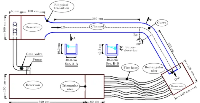
Figure 1. Geometrical shape of the ume used in this paper. Table 1. Dierent experimental hydraulic properties. No. of
test
Normal depth y (cm)
Discharge Q (l/s)
Velocity (m/s)
Froude number
Reynolds number
1 4.5 5 0.273 0.42 12460
2 6 7.8 0.321 0.42 18460
3 9 13.6 0.374 0.40 28940
4 12 19.1 0.394 0.36 36860
5 15 25.3 0.419 0.34 44705
6 17.6 30.8 0.435 0.33 50830
research on 60 sharp bend channels in the hydraulics
laboratory of Ferdowsi University in Mashhad. The channel under examination had three parts: the 360 cm long straight inlet channel, the 60 curved channel
with 60.45 cm central radius of the bend (Rc), and
the 180 cm long straight outlet channel. The cross sections of the intended ume were square shaped with a width (b) of 40.3 and a height (h) of 40.3 cm, and the bed and the walls were made of Plexiglas. The geometrical shape of the ume is shown in Figure 1. Six dierent hydraulic conditions are considered in the experiments in this paper, as shown in Table 1. A one-dimensional propeller velocity-meter and a micro-meter (mechanical bathomicro-meter) are used to read the axial velocities and water surface depth, respectively, in the ume. The precision of the micro-meter is 0.1 mm and the precision of the propeller is 2 cm/s. The velocity-meter is located by Vernier ruler and analog caliper in the transverse direction with precision of 0.5 mm and depth direction with precision of 0.1 mm, respectively [43]. Finally, the propeller measures
the velocity in ow direction (axial velocity or radius velocity). Also, in internal bend cross sections (e.g., 10, 20, 30, 40, 50, and 60cross sections), the ow
velocity is read in channel axis direction by velocity-meter. In internal cross sections, the longitudinal and transversal velocities (Vx and Vy) are found using the
velocity obtained by velocity-meter, which is broken in X and Y directions.
2.2. Numerical models
2.2.1. Computational Fluid Dynamics (CFD) model Dierent control volumes are considered for the whole ow elds in FLUENT software. Then, the Navier-Stokes governing equation (in uid ow) is integrated in each control volume. The integrated algebraic equation in each control volume is calculated and separated via dierent plans. The simulation of the ow in every 60
bend under study is three-dimensional, the Volume of Fluid (VOF) multiphase model is used, and the \ow in open channel" option is activated [44]. In order to complete the preparation process of the numerical
model, the \PRESTO" plan is used for expanding the pressure, the \PISO" plan for velocity-pressure coupling, the \Quick" plan for momentum and volume fraction, and the \Second Order Upwind" for separat-ing the displacement sentences. Also, relaxation coef-cients below one are used for pressure, momentum, turbulence kinetic energy (k), and turbulence kinetic energy dissipation rate (") to prevent the divergence of the solution. The essential time step for solving the equations is considered to be equal to 0.001 with regards to the divergence process of this simulation.
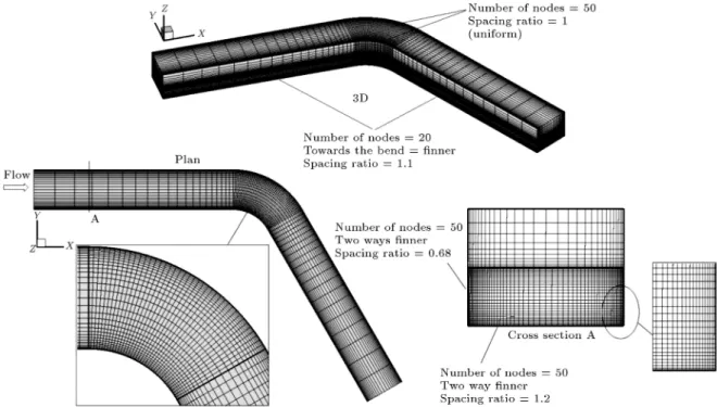
Gambit software is used to create the geometry and meshing of the solution eld. To adjust the meshing in bend, the grid near the oor, walls, interior of the bend, and the interface surface between two phases, ner and coarser grids in the rest of the network is considered. Overall, the considered grid sizing has 225000 nodes (50 50 90 nodes in width, depth, and length, respectively) for a 60 bend. Figure 2
shows a view of the gridding 60 bend model. Also,
the dimensions of the used mesh in CFD are presented in Figure 2 in detail.
In the present paper, the \Velocity Inlet" bound-ary condition is used separately for water and air in the inlet as the air velocity is considered to have a very small value (0.0001 m/s), and ow velocity is applied in accordance with each laboratorial setup (Table 1). Furthermore, the \Pressure Outlet" is considered for the outlet and free surface of channel as boundary condition. Also, in the channel inlet the \Pressure Inlet" is considered as boundary condition for two phase ow of uid and air (with atmospheric pressure
Figure 3. Computational scope and boundary conditions for 60bend.
value). The oor and walls of the channel undergo the \Wall" boundary condition using standard wall function. A scheme of the computational scope and the boundary conditions governing the 60 bend is
presented in Figure 3.
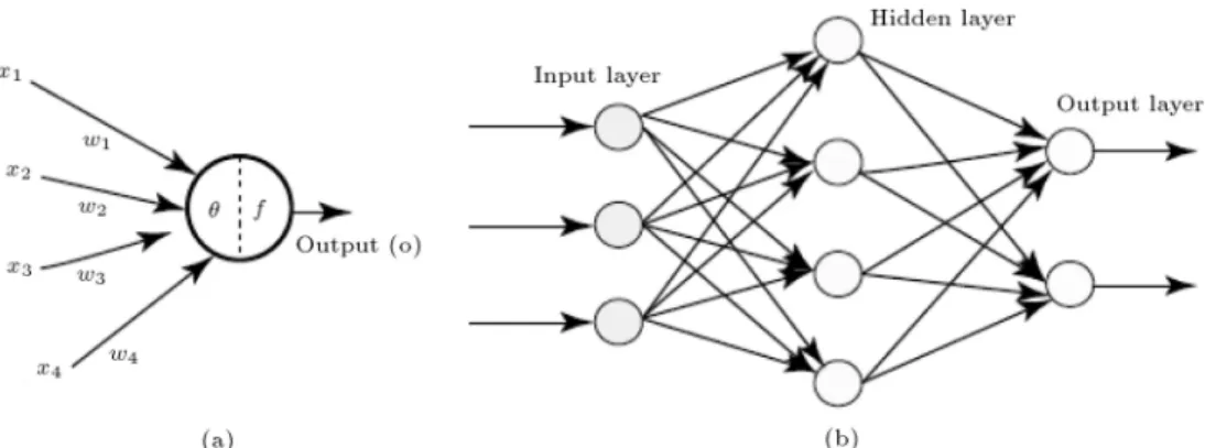
2.2.2. Overview of articial neural network model Articial neural networks were inspired by the perfor-mance system of human brain. The most important component of these networks is named neuron. The ANN models are arranged in three dierent input, hidden, and output layers. Generally, there are only one input layer, one output layer, and one or more hidden layers. In the present paper, the articial intelligence tool in MATLAB software is used to design a Multi-Layer Perceptron Neural Network (MLP NN) model in prediction of ow variables in curved channel. Figure 4 shows a general view of this network. The specic weights are used to connect the neurons to each other in designing the network. The input layer intro-duces the input variables to the model with neurons and transfers them to the hidden layer. The neurons
Figure 4. Architecture of (a) an articial neuron and (b) a multi-layer articial neural network.
of input layer are collected by hidden neurons using weighted summation. Also, the activation function is used to make nonlinear mapping between input and output layers. In the present paper, the MLP model uses sigmoid activation function [29,45, and 46]. The numbers of input and output model variables are considered as the neuron numbers of input and output layers, respectively. Determination of weight coecient in MLP model is named training. In this study, the \back propagation" algorithm is used for training process through Levenberg-Marquardt (LM) method [47]. The \stop" training for the criteria is considered to consist in 100 epochs, which is achieved when the model converges completely [19,48]. The error level between ANN model and the observed data is considered to determine the number of the epochs (iterations). Model convergence should be achieved for each number of iterations. In this study, the number of iterations is considered 100 for MLP model.
Moreover, for water surface depth prediction, the numbers of neurons in input and output layers are considered 3 and 1, respectively. Also, two hidden layers are selected associated with 10 neurons in each layer. In the velocity prediction model, the neurons numbers in input, one hidden, and output layers are considered 3, 40, and 1, respectively.
2.2.3. Overview of Support Vector Machines (SVM) model
Support Vector Machines (SVM) modeling was rstly introduced by Vapnik [49] based on statistical learning theory. The SVM is utilized in classication and regression problems known as SVC and SVR (in cur-rent study), respectively. The SVM maps the sample space to a high-dimensional feature space to discover an optimal segregating hyper plane [50]. It avoids the curse of dimensionality and over-tting that occur in traditional machine learning techniques such as Articial Neural Network (ANN). The calculation of error through SVR modelling is based on structural risk minimization principle, which is dierent from
empirical risk minimization principle employed in con-ventional neural networks [49]. Therefore, SVR models reduce the generalization error rather than the training error.
The main objective in modelling by SVR is the estimation of functional dependency, f (~x), a set of data points, X = (~x1; ~x2;:::; ~xl) 2 Rn, and target
variable Y = (~y1; ~y2;:::; ~yl) (yi2 R). By assuming that
all samples are produced from an unknown function of probability distribution P (~x; y):
F = ffjf (~x) = (~w; ~x) + B : ~w 2 Rn; Rn! Rg ; (1)
where B and ~w are coecients which are dierent for each problem. The function f(~x), which minimizes the risk function, should be determined. It is dened as:
R [f (~x)] = Z
l (y f (~x) ; ~x) dP (~x; y); (2) where l is the loss function utilized to calculate the deviation between estimated f(~x) and target values. Considering the unknown probability distribution func-tion of P (~x; y), R [f (~x)] cannot be minimized directly. Thus, the empirical risk function is calculated as:
Remp[f (~x)] =N1 N
X
i=1
l (yi f (~xi)): (3)
This approach is not recommended without any regu-larization. Thus, a regularized risk function with the smallest sharpness among the whole functions, which minimizes the empirical risk function, is utilized as follows:
Rreg[f (~x)] = Remp[f (~x)] + k~wk2; (4)
where is a positive constant. The additional term in the above-mentioned equation decreases the model space and then, controls the complexity of the problem solution. Therefore, this expression can be considered in the following form:
Rreg[f (~x)] = C
X
xi2X
l"(yi f (~xi)) +12k~wk2; (5)
known as penalty factor (additional capacity control), and should be determined beforehand. The parameter C shows the inuence of the trade-o between weight vector jjwjj and an approximation error. Increase in this parameter penalizes larger errors, leading to reduction of estimation error, which is attained through increasing the regression vector. The loss function, which is known as "-intensive loss function, is consid-ered as follows:
l"(yi f (~xi)) =
(
0 for jyi f (~xi)j<"
jyi f (~xi)j otherwise (6)
This function has the benet that it does not require all the input data for explanting the regression vector ~w. When the function is synthesized with the regu-larization term 0:5 k~wk2, it behaves as a biased estimator. Determination of " is simpler than C and it is mostly given as the favourable percentage of the output values (yi). Therefore, the nonlinear function
is given through a function that minimizes Eq. (5), subject to Eq. (6), in the following form [49]:
f (x) =XN
i=1
(a
i ai) K (x; xi) + B; (7)
where a
i and aiare the Lagrange multipliers, K(x; xi)
is the kernel function, and B is the bias. Assuming that the average of data is zero, which can be attained by pre-processing, the bias is dropped.
The kernel function provides operations which act in the input space rather than in the potential feature space. Thus, a kernel function in the input space is comparable with an inner product in the feature space. Generally, the kernel functions handled by the SVM are linear Radial Basis Functions (RBF) in sigmoid and polynomial models. RBF is the most commonly used kernel function, which leads to accurate prediction as well as simplicity and credibility with the hydraulic problems [51-54]. This kernel function is employed in this study, which is computed as follows:
K (x; xi) = exp
kx xik2
; (8)
where is the kernel parameter and equal to 1=(22).
Choosing , ", and C parameters aects the prediction accuracy, which is made by RBF kernel function. The optimum values of constant parameters in the developed SVM for ow depth and velocity eld are (C = 8; " = 0:005; = 0:01) and (C = 3; " = 0:05; = 0:01), respectively, which are obtained by trial and error.
2.2.4. Datasets
The input variables for predicting water surface and velocity are 3 numbers that are coordinates of points
in the X and Y directions, and ow discharge (Q) and the output variables are the corresponding velocity and water surface depths of these points.
The axial velocity or radial velocity is measured by experiments in all cross sections. Before the bend cross section (40 cm before the bend), in similar experimental measurements, the velocity predicted by CFD is axial velocity (velocity in ow direction), Vx, of which the corresponding experimental data is
considered for SVM modelling. After the bend cross sections (40 cm and 80 cm after the bend) and internal cross sections (e.g., 10, 20, 30, 40, 50, and 60),
the velocities in X and Y directions (Vx and Vy) are
predicted by CFD model; then, the catching up of these two velocities (Vx and Vy) is calculated and VT (total
velocity or obtained axial velocity) is considered for drawing velocity prole distributions. In these sections, the axial velocity measured by the experimental model in each transversal point is considered for ANN and SVM modelling.
In velocity and water depth prediction models, 130 experimental data are selected for each discharge in 13 transverse points located on 10 dierent cross sections, namely 40 cm before the bend; on 0, 10,
20, 30, 40, 50, and 60; and 40 and 80 cm after the
bend. Thus, in 6 discharges ((Q): 5, 7.8, 13.6, 19.1, 25.3, and 30.8 (l/s)), there are a total of 780 (130 6) data for each velocity and ow depth prediction.
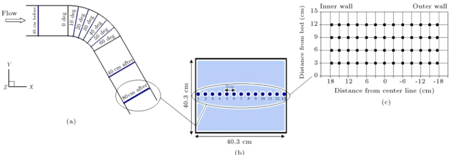
In the present paper, out of 780 data, 546 data (70% of the whole data) and 234 data (30% of the whole data) are chosen for training and testing models, respectively, in each velocity and ow depth prediction. Other methodologies such Genetic Algorithm (GA) and a Self-Organizing Map (SOM) for dividing data are suggested, which reduce the error indices in the conventional data division techniques [55]. The used velocity values are depth averaged velocity in each point. Figure 5 shows the coordinates of transverse points and dierent cross sections used for measure-ment of velocity and water surface in 60 bend.
2.3. Statistical measurement of model performance
In order to evaluate the dierence between the obtained and actual values, there are many methods to calculate the error: absolute error indices such as Root Mean Square Error (RMSE), Mean Absolute Error (MAE), Mean Absolute Relative Error (MARE), and Mean Absolute Percentage Error (MAPE). These indices represent the dierences between observational and modeled parameters in the same units and scales. The closer the values of these indices to zero, the higher the accuracy of the models will be. Correlation coecient (R) is an index of descriptive statistics, which describes the degree to which two variables are correlated and the direction of the correlation. The
Figure 5. (a) 10 dierent cross sections, (b) 13 transverse points, and (c) the point coordinates in 4 distances from the channel bed to measure the velocity and water depth in 60bend.
more homogeneous the changes of the two variables, the higher the values of the correlation coecients will be. The absolute value of the correlation coecient, that is, the correlation coecient without the sign (+ or { ), indicates the strength of the correlation of the two variables. Generally, the closer the value obtained by the model to 1, the closer it will be to the actual value and the better the performance of the model will be. Another index, namely, Bias, is applied to determine the performance of the model in estimating the values in comparison with observational data (overestimation or underestimation). The negative and positive values of Bias index represent the underestimation and over-estimation of model performance, respectively. The mentioned indices are calculated in accordance with the following equations:
RMSE = N1
N
X
i=1
(Xobsi Xesti)2
!1 2
; (9)
MAE = N1
N
X
i=1
jXobsi Xestij; (10)
MAP E (%) = 100 N
N
X
i=1
jXobsi Xestij
Xobsi
; (11) MARE =N1 XN
i=1
jXobsi Xestij
Xobsi
; (12)
R =
N
P
i=1 Xobsi Xobsi
: Xesti Xesti
s
N
P
i=1 Xexpi Xexpi
2:PN
i=1 Xesti Xesti
2
; (13)
Bias = N1 XN
i=1
(Xesti Xobsi); (14)
Xobsi is the observed parameter in the
above-mentioned equations, Xestiis the parameter estimated
by the models, Xobsiis the mean observed parameter,
Xesti is the mean parameter estimated by the model,
and N is the number of the parameters. 3. Results and discussions
3.1. Performance evaluation of velocity prediction models
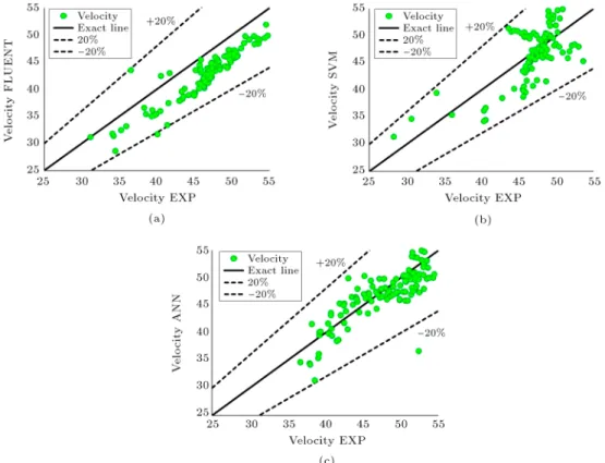
Figure 6 shows the scatter plot graphs for the velocity values predicted by FLUENT, SVM, and ANN models in comparison with the experimental values. It can be seen that the results of all the three models have an acceptable level of consistency with the observational values. All the data are within 20% range of the error line for all the three models. However, studying this gure carefully will make it clear that most of the data are around the exact line in the ANN model and they are not widely scattered. The data are more scattered in FLUENT and SVM models. Almost all of them are between the exact line and 20% error line in the FLUENT model and between the +20% and 20% error lines in the SVM model. Most of them are concentrated around the exact line in the FLUENT model and the SVM results are located farther from the exact line. Therefore, the SVM model is less precise than the other models.
All the dierent statistical indices for predicting the velocity parameters and comparing the FLUENT, ANN, and SVM models are shown in Table 2. Note that all these indices are related to the whole datasets (train + test dataset) for SVM and ANN models. Regarding the velocity-predicting models, it is clear that the MARE relative error index of the ANN model, which is equal to 0.055, is smaller than those of the rest of the models. It is followed by SVM with a relative error of 0.069 and then comes the FLUENT model with a relative error of 0.089. The MARE index,
Figure 6. The scatter plot graphs for the velocity values predicted by (a) FLUENT, (b) SVM, and (c) ANN models in comparison with the experimental values.
Table 2. Assessing the performance of FLUENT, SVM, and ANN models in predicting the velocity in comparison with the experimental values through using dierent statistical indices.
Variable Models RMSE (cm) MAE (cm) MARE (cm) R Bias (cm)
FLUENT 4.500 4.251 0.089 0.95 -4.124
Velocity prediction SVM 4.411 3.354 0.069 0.68 -0.575
ANN 3.497 2.642 0.055 0.81 0.098
which is chosen as the appropriate evaluation scale for the comparison of models, represents the relative dierences between the predicted and observed values. According to MARE values, the ANN model has the highest accuracy among other models and is the best model in the present paper. For making more clear comparison between presented models, other indices are considered. The MAE index represents the abso-lute dierence values between predicted and observed values. The absolute error values for this index also follow the same trend in all three models. The MAE error values are equal to 2.642, 3.354, and 4.251 in ANN, SVM, and FLUENT models, respectively. Based on the values, the MAE has the same scale and unit; therefore, the dierence between predicted and observed values in ANN model has the smallest value among the models (2.642cm). Thus, it can be said that, similar to MARE value, the MAE value in ANN model has the smallest amount among the models, which indicates the slight dierence between predicted
and observed values (almost 2 cm) and high eciency of ANN model. In addition to the dierence between predicted and observed values, the performance of the models in estimating either higher and lower values than observed values is signicant in evaluation. In this respect, the Bias index shows the overestimation and underestimation of the models with negative values indicating underestimation and the positive ones indi-cating overestimation. According to the Bias values, both the FLUENT and SVM models predict lower and the ANN model forecasts higher values than that of the experimental model. Therefore, it can be concluded that the ANN model is overestimating and FLUENT and SVM models are underestimating. Another error index is RMSE, which is suitable for the performance of models with higher data values. The dierence between predicted and observed values in this scale is squared and higher RMSE values represent higher error and consequently, higher dierence in the data. In velocity prediction models, the ANN model with the
smallest RMSE value (almost 3.5 cm) performs more eciently than other models. The FLUENT model with the highest RMSE value (4.5 cm) represents the weakest performance among all models, especially with high data values. The R value presents the correlation between the data of the model and the experimental values, and the correlation of two variables as well as the direction of the correlation. This value is greatest in the FLUENT model among all of them (R = 0:952). However, it can be seen from Figure 6(a) that the predicted data by FLUENT model are scattered between the exact line and the 20% error line. In this model, the trend line is parallel to the exact line, and despite the fact that the R value in this model is close to one, it cannot be said that this model is the most accurate model in prediction of the ow velocity. Considering the large error values in Table 2, this model performs the worst in comparison with ANN and SVM models in the prediction of ow velocity. This model predicts all velocity values less than experimental ones with error values of 10-20%. Almost the whole data are predicted by the FLUENT model in this error range. In addition, the high amounts of Bias value (also negative signs) approve the underestimating performance of the FLUENT model. This can be considered as a disadvantage for the FLUENT model that it estimates lower than a certain error value in prediction of the ow pattern. Despite smaller values of R in ANN and SVM models than in FLUENT model, the lower values of error indices and more logical data distribution in
scatter graphs between error lines and exact line in these models than in the FLUENT model represent the high eciency of these models. However, as it was mentioned previously, the ANN model with the lowest error values is the best model in the velocity prediction in this study.
3.2. Performance evaluation of water surface depth prediction models
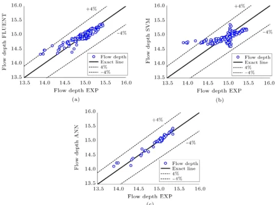
The scatter plot graphs of the water depths predicted by these models are shown in Figure 7. The water surface depth values predicted by all the three models have an acceptable agreement with the observed data. The data are concentrated around the exact line in all the three models. However, careful examination of the images will clarify that all the data are within the 5% error line range in the ANN model. After that, in the FLUENT model, a few data fall outside the +5% error line and then, in the SVM model, more data exceed this error line.
The error indices are gathered in Table 3 for mak-ing better comparison between all models for the whole datasets. It could be seen in the ow depth predicting models that the dierence between the predicted values and the experimental values is smaller for the ANN model than for the other models (MAE = 0:052 cm). The SVM and FLUENT models have smaller abso-lute error values, respectively, after the ANN model (0.105 cm and 0.169 cm for FLUENT and SVM models, respectively). Also, as in the velocity prediction, the
Figure 7. The scatter plot graphs for the water depth values predicted by (a) FLUENT, (b) SVM, and (c) ANN models in comparison with the experimental values.
Table 3. Assessing the performance of FLUENT, SVM, and ANN models in predicting the ow depth in comparison with the experimental values.
Variable Models RMSE (cm) MAE (cm) MARE (cm) R Bias (cm)
FLUENT 0.135 0.105 0.007 0.914 -0.012
Flow depth prediction SVM 0.228 0.169 0.011 0.696 -0.028
ANN 0.074 0.052 0.004 0.999 0.006
relative error is smaller in the ANN model than in the other models when predicting the water depth (MARE = 0:004). The relative error index in ANN model is improved almost 43% and 64% in comparison with the FLUENT and SVM models, respectively. In comparison with the velocity prediction models, the ANN model has the smallest absolute RMSE value (RMSE = 0:074). Therefore, this model also has an acceptable eciency in prediction of high ow depth values. On the other hand, the correlation coecient (which is described as the relationship between the predicted and observed values) in ANN model has high values (almost close to 1) that conrm the high accu-racy of ANN model. Thus, it can be concluded that the ANN model with the lowest error index is the best model in ow depth prediction among all the models. The FLUENT and SVM models predict the water sur-face with underestimation and the ANN model predicts the water surface with overestimation. The Bias value in ANN model is close to 1, which approves the high accuracy of this model in ow depth prediction. The R values of FLUENT and SVM models are smaller (0.914 and 0.696) than that of the ANN model (0.999). In SVM model, the R index value is described as the weakness of the model in water depth prediction. 3.3. Transverse depth-averaged velocity
proles
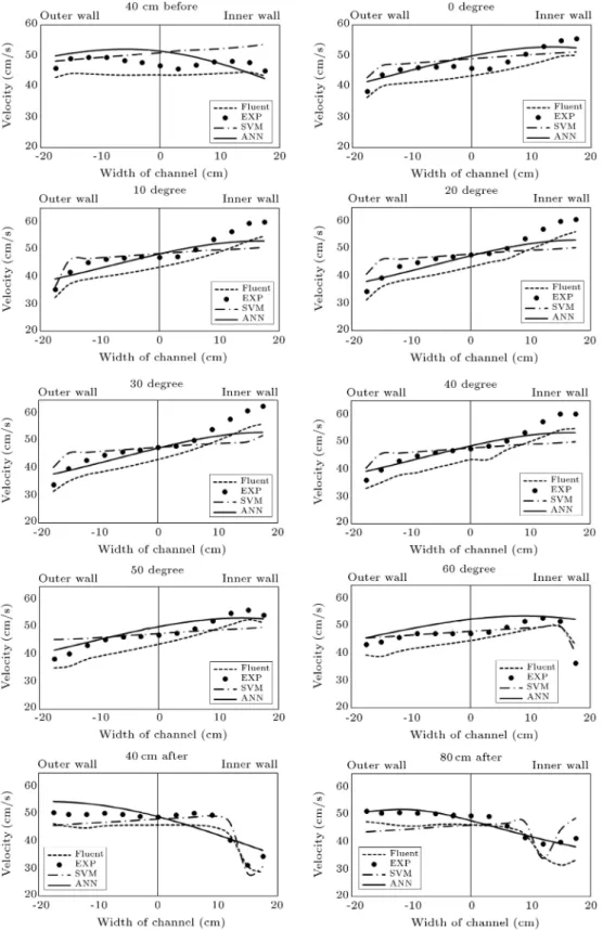
Figure 8 shows the transverse proles of the depth averaged velocity in 25.3 l/s discharge in dierent
transverse cross sections by all the three models. It could be seen in these graphs that all the three models, i.e. ANN, SVM, and FLUENT, perform well in predicting the velocity. All the three models are very well able to simulate the longitudinal velocity values in various cross sections in such a manner that the maximum velocity is placed, and maintained, in the inner wall of the channel up to the nal cross sections of the bend. At the 60 cross section, the maximum
velocity gradually separates from the inner wall of the channel and transfers to the channel axis; then, it is totally placed outside the channel in the cross sections located after the bend. It could be seen in these gures that all the three models perform well in predicting the velocity pattern, but they are somehow dierent when it comes to predicting the velocity values. Table 4 shows the RMSE and MAPE error values for these cross sections in all three models. It could be seen in the table that with smaller error values, the ANN model performs averagely better than the other two models (RMSE = 3:31 and MAP E = 5:57%). In the following are the SVM model and the FLUENT model in predicting the velocity with MAPE values of 7.14% and 8.69%, respectively. The relative error index in ANN model, almost 5%, represents the high accuracy of the model in velocity prediction, especially 80 cm after the bend cross section (MAPE value of almost 5% and RMSE of almost 3 cm) unlike SVM and FLUENT models with high error values in this cross section. The high value of relative error in SVM model in
Table 4. Calculating the RMSE and MAPE errors for depth averaged velocity by FLUENT, ANN, and SVM models in comparison with the experimental values in 25.3 l/s discharge in dierent cross sections.
FLUENT ANN SVM
Cross section RMSE (cm) MAPE (%) RMSE (cm) MAPE (%) RMSE (cm) MAPE (%)
40 cm before 3.96 7.88 3.23 5.95 4.14 6.59
0 3.97 7.82 2.68 4.57 2.90 5.45
10 5.04 9.95 3.48 5.96 4.50 6.51
20 4.81 9.74 3.64 5.74 5.44 8.48
30 5.12 10.14 4.20 6.30 5.80 8.89
40 4.97 10.06 3.24 4.71 5.34 8.24
50 4.03 8.29 2.28 4.19 3.89 6.20
60 4.13 8.52 5.40 7.61 1.88 3.13
40 cm after 4.04 8.07 3.92 7.09 3.23 6.62
80 cm after 4.69 9.12 1.62 2.94 5.33 11.29
Figure 8. The transverse depth averaged velocity distribution in dierent cross sections with 25.3 l/s discharge by three ANN, SVM, and FLUENT models.
80 cm after the bend cross section (MAP E = 11:29%) demonstrates the low accuracy of this model in velocity prediction. The ANN model has smaller relative error in 40 and 50cross sections than other models (almost
4%), which represents the high performance of the
model in these cross sections. However, the RMSE error is generally lower in ANN model for all cross sections, which shows the high prociency of it in predicting high values of velocity. Finally, it can be concluded that the ANN model has smaller error values
and performs better than the other two models in all the cross sections and it is the best model in velocity prediction at transverse cross sections. However, The SVM model is more precise for the 60 cross section
and for the cross section located 40 cm after the bend, especially in prediction of high velocity values, which leads to a lower RMSE value (1.88 cm).
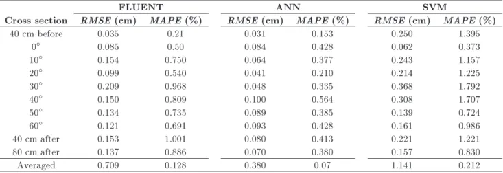
3.4. Transverse water surface proles
Table 5 shows RMSE and MAPE error values for the transverse proles of the water surface in dierent cross sections by all the three FLUENT, ANN, and SVM models with 25.3 l/s discharge in comparison with the experimental values. All the three models have moderate RMSE and MAPE values and thus, perform better than the velocity prediction models. According to Table 5, with smaller error values (RMSE = 0:380 and MAP E = 0:07%), the ANN model performs better than the other two models as well as the velocity models. FLUENT and SVM models perform at an acceptable level after ANN (MAP E = 0:128% and 0.212%, respectively). The lower RMSE value in ANN model (almost under 0.1 cm) illustrates the high accuracy of this model in predicting of all amounts of ow depth, especially before the cross sections and in the internal cross sections of the bend (20 and 30
cross sections). The SVM and FLUENT models have high relative errors, almost 67% and 45% higher than that of the ANN model, respectively, which show their lower accuracy. The FLUENT model with more RMSE values (almost higher than 0.1 cm) has lower eciency in predicting of high values of ow depth than the other model. In general, the ANN model with a very small relative error index (0.07%) and lower RMSE value (high performance in estimating ow depths with high amounts) is the best model in this section.
Figure 9 shows the error contours in the bend plan as e = (hexp hmodel=hexp) in percentage for
predicting the water depth by the all three models in comparison with the experimental results. The error range is smaller in the ANN model than in the other two models in the entire bend (-1.2 to 1.6). The error value is lower in the inner wall in the ANN model than in the SVM and FLUENT models in such a manner that the ANN model is the best model in the cross sections within the bend, enjoying an error value of approximately zero. The FLUENT model comes after with an error value of almost 1% and then comes the SVM model with an approximate error value of 3-4%. The error value is smaller in the outer wall (contraction zone) than in the inner wall (separation zone) in all the three models (it is almost half that in the inner wall in the FLUENT model, almost one third in the SVM model, and 0.4 in the ANN model). Therefore, it could be stated that the error values in the zones with maximum velocities are higher than those in the zones with minimum velocities. Also, in three ANN, SVM and FLUENT models, the lower error values in the sections after the bend can be negligible. The error value is insignicant in the cross sections after the bend in all the three models in such a manner that it is between 0:4 and 0.4 in the ANN model and it is almost zero in the cross sections near the exit. In all models, the error values in initial bend cross sections are almost equal to zero. The error contours are more concentrated in the inner wall than in the outer wall of the channel in all three models, which is due to the density of the streamlines in this wall.
4. Conclusion
In this study, two numerical techniques, namely com-putational uid dynamics and soft computing, were investigated in the prediction of the three-dimensional ow pattern on curves. Also, due to the complexity of the ow pattern in sharp curves, a 60 sharp bend
Table 5. Calculating the RMSE and MAPE errors for water surface depth prediction by the models in comparison with the experimental values in 25.3 l/s discharge in dierent cross sections.
FLUENT ANN SVM
Cross section RMSE (cm) MAPE (%) RMSE (cm) MAPE (%) RMSE (cm) MAPE (%)
40 cm before 0.035 0.21 0.031 0.153 0.250 1.395
0 0.085 0.50 0.084 0.428 0.062 0.373
10 0.154 0.750 0.064 0.377 0.243 1.157
20 0.099 0.540 0.041 0.210 0.214 1.225
30 0.209 0.968 0.048 0.335 0.368 1.792
40 0.150 0.809 0.100 0.564 0.308 1.707
50 0.134 0.735 0.089 0.385 0.139 0.724
60 0.121 0.691 0.093 0.428 0.161 0.986
40 cm after 0.153 1.001 0.080 0.413 0.221 1.221
80 cm after 0.137 0.886 0.070 0.380 0.157 0.830
Figure 9. Water surface prediction error contours in the bend plan with e = (hexp hmodel=hexp) in percentage by all the
three models: (a) FLUENT, (b) SVM, and (c) ANN.
was chosen and extensive experimental research by the authors was performed on it. The advantage of this study is that experimental studies were done in 6 dierent hydraulic conditions and the experimental results were used for training and testing the articial intelligence models. The results showed that, compared to experimental values, all the three ANN, SVM, and CFD models performed well with acceptable errors in prediction of two velocity and water depth variables. ANN model predicted both the velocity and water surface variables with lower error value and was the superior model. FLUENT model estimated velocity values with errors about 10-20% and showed the lowest accuracy. In despite of this, it gave us the certainty that this model in velocity prediction in the curved channels had a certain achievement. However, FLUENT model, following the ANN model, was the best, because using turbulence model nonlinear, k " (RNG), led to more accurate prediction of the water free surface. In general, ANN and SVM methods, with lower time and cost than the expensive experimental methods and CFD model, are more appropriate. However, the CFD model, because of complex Navier-Stokes equations governing the ow curves, and experimental
methods, due to the governing physics in the ow, are important as well. Other data division methods have been proposed to decrease and increase the error values and model accuracy, respectively.
References
1. Baghlani, A. \Simulation of ow and mass dispersion
in meandering channels", Scientia Iranica, Transac-tions A: Civil Engineering, 19, pp. 1463-1472 (2012).
2. Shukry, A. \Flow around bends in an open ume",
Transactions, ASCE, 115, pp. 751-788 (1950).
3. Rozovskii, I.L. \Flow of water in bends of open
channels", Israel Program for Science Translation, Jerusalem, pp. 1-233 (1961).
4. DeVriend, H.J. and Geoldof, H.J. \Main ow velocity
in short river bends", Journal of Hydraulics Engineer-ing, 109(7), pp. 991-1011 (1983).
5. Bergs, M.A. \Flow processes in a curved alluvial
channel", Ph.D. Thesis, The University of Iowa (1990).
6. Ye, J. and McCorquodale, J.A. \Simulation of curved open channel ows by 3D hydrodynamic model", Journal of Hydraulic Engineering- ASCE, 124(7), pp. 687-698 (1998).
7. Blanckaert, K. and Graf, W.H. \Mean ow and tur-bulence in open channel bend", Journal of Hydraulic Engineering, 127(10), pp. 835-847 (2001).
8. Barbhuiya, A.K. and Talukdar, S. \Scour and three
dimensional turbulent ow elds measured by ADV at a 90horizontal forced bend in a rectangular channel", Flow Measurement and Instrumentation, 21, pp. 312-321 (2010).
9. Ramamurthy, A., Han, S., and Biron, P.
\Three-dimensional simulation parameters for 90open chan-nel bend ows", Journal of Computing in Civil Engi-neering. ASCA, 27(3), pp. 282-291 (2013).
10. Gholami, A., Akhtari, A.A., Minatour, Y., Bonakdari, H., and Javadi, A.A. \Experimental and numerical study on velocity elds and water surface prole in a strongly-curved 90 open channel bend", Engineering Applications of Computational Fluid Mechanics, 8(3), pp. 447-461 (2014).
11. Leschziner, M.A. and Rodi, W. \Calculation of
strongly curved open channel ow", Journal of the Hydraulics Division, 105(10), pp. 1297-1314 (1979).
12. Naji, M.A., Ghodsian, M., Vaghe, M., and Panahpur,
N. \Experimental and numerical simulation of ow in a 90bend", Flow Measurement and Instrumentation, 21(3), pp. 292-298 (2010).
13. DeMarchis, M. and Napoli, E. \3D numerical
sim-ulation of curved open channel ows", Proceedings of 6th International Conference on Water Resources, Hydraulics & Hydrology, pp. 86-91, Chalkida, Evia Island, Greece, May 11-13 (2006).
14. Bodnar, T., Prihoda, J. \Numerical simulation of
turbulent free-surface ow in curved channel", Flow, Turbulence and Combustion, 76, pp. 429-442 (2006).
15. Gholami, A., Bonakdari, H., and Akhtari, A.A.
\As-sessment of water depth change patterns in 120 sharp bend using numerical model", Water Science and Engineering, 4(9), pp. 336-344 (2016).
16. Bonakdari, H., Larrarte, F., and Joannis, C. \Eect
of a bend on the velocity eld in a circular sewer with free surface ow", Proceeding of 6th International Conference on Sustainable Techniques and Strategies in Urban Water Management, pp. 1401-1408, Lyon, France, June 24-28 (2007).
17. Zeng, J., Constantinescu, G., Blanckaert, K., and
Weber, L. \Flow and bathymetry in sharp open-channel bends: Experiments and predictions", Water Resources Research, 44(9), w09401, pp. 1-22 (2008).
18. Gholami, A., Bonakdari, H., and Akhtari, A.A.
\De-veloping nite volume method (FVM) in numerical simulation of ow pattern in 60open channel bend", Journal of Applied Research in Water and Wastewater, 3(1), pp. 193-200 (2016).
19. Kisi, O. and Cigizoglu, H.K. \Comparison of dierent ANN techniques in river ow prediction", Civil Engi-neering Environment System, 14, pp. 211-231 (2007).
20. Najafzadeh, M. and Azamathulla, H.M. \Neuro-fuzzy
GMDH to predict the scour pile groups due to waves", Journal of Computing in Civil Engineering, 29(5), 04014068 (2013).
21. Najafzadeh, M., Barani, G.A., and Hessami Kermani,
M.R. \Estimation of pipeline scour due to waves by GMDH", Journal of Pipeline Systems Engineering and Practice, 5(3), 06014002 (2014).
22. Najafzadeh, M. and Zahiri, A. \Neuro-fuzzy
GMDH-based evolutionary algorithms to predict ow discharge in straight compound channels", Journal of Hydrologic Engineering, 20(12), 04015035 (2015).
23. Najafzadeh, M., Barani, G.A., and Hessami-Kermani,
M.R. \Evaluation of GMDH networks for prediction of local scour depth at bridge abutments in coarse sedi-ments with thinly armored beds", Ocean Engineering, 104, pp. 387-396 (2015).
24. Najafzadeh, M., Etemad-Shahidi, A., and Lim, S.Y.
\Scour prediction in long contractions using ANFIS and SVM", Ocean Engineering, 111, pp. 128-135 (2016).
25. Najafzadeh, M., Balf, M.R., and Rashedi, E.
\Pre-diction of maximum scour depth around piers with debris accumulation using EPR, MT, and GEP mod-els", Journal of Hydroinformatics, 18(5), pp. 867-884 (2016).
26. Najafzadeh, M. and Sattar, A.M. \Neuro-fuzzy GMDH
approach to predict longitudinal dispersion in water networks", Water Resources Management, 29(7), pp. 2205-2219 (2015).
27. Gholami, A., Bonakdari, H., Ebtehaj, I., and Akhtari, A.A. \Design of an adaptive neuro-fuzzy computing technique for predicting ow variables in a 90 sharp bend", Journal of Hydroinformatics, 19(4), jh2017200 (2017).
28. Gholami, A., Bonakdari, H., Zaji, A.H., Fenjan,
S.A., and Akhtari, A.A. \New radial basis function network method based on decision trees to predict ow variables in a curved channel", Neural Computing and Applications, 30(9), pp. 2771-2785 (2018).
29. Gholami, A., Bonakdari, H., Zaji, A.H., Ajeel Fenjan, S., and Akhtari, A.A. \Design of modied structure multi-layer perceptron networks based on decision trees for the prediction of ow parameters in 90 open-channel bends", Engineering Applications of Compu-tational Fluid Mechanics, 10(1), pp. 193-208 (2016).
30. Gholami, A., Bonakdari, H., Ebtehaj, I., Shaghaghi, S., and Khoshbin, F. \Developing an expert group method of data handling system for predicting the geometry of a stable channel with a gravel bed", Earth Surface Processes and Landforms, 42(10), pp. 1460-1471 (2017). DOI: 10.1002/esp.4104
31. Shaghaghi, S., Bonakdari, H., Gholami, A., Ebtehaj, I., and Zeinolabedini, M. \Comparative analysis of GMDH neural network based on genetic algorithm and particle swarm optimization in stable channel design", Applied Mathematics and Computation, 313, pp. 271-286 (2017).
32. Kaveh, A. and Nasrollahi, A. \Charged system search and particle swarm optimization hybridized for opti-mal design of engineering structures", Scientia Iranica, Transactions A: Civil Engineering, 21, pp. 295-305 (2014).
33. Ebtehaj, I., Bonakdari, H., Zaji, A.H., Azimi H., and Shari, A. \Gene expression programming to predict the discharge coecient in rectangular side weirs", Applied Soft Computing, 35, pp. 618-628 (2015).
34. Karimi, S., Bonakdari, H., and Gholami, A. \Determi-nation discharge capacity of triangular labyrinth side weir using multi-layer neural network (ANN-MLP)", Current World Environment, 10(Special issue 1), pp. 111-119 (2015).
35. Zarif Sanayei, H.R., Talebbeydokhti, N., and Morad-khani, H. \3D estimation of metal elements in sedi-ments of the Caspian Sea with moving least square and radial basis function interpolation methods", Scientia Iranica, Transactions A: Civil Engineering, 22, pp. 1661-1673 (2015).
36. Bonakdari, H., Baghalian, S., Nazari, F., and Fazli, M. \Numerical analysis and prediction of the velocity eld in curved open channel using articial neural network and genetic algorithm", Engineering Applications of Computational Fluid Mechanics, 5(3), pp. 384-396 (2011).
37. Sahu, M., Jana, S., Agarwal, S., and Khatua, K.K.
\Point form velocity prediction in meandering open channel using articial neural network", 2nd Inter-national Conference on Environmental Science and Technology, 6, pp. 209-212, Singapore: IACSIT Press (2011).
38. Gholami, A., Bonakdari, H., Zaji, A.H., and Akhtari, A.A. \Simulation of open channel bend characteristics using computational uid dynamics and articial neu-ral networks", Engineering Applications of Computa-tional Fluid Mechanics, 9(1), pp. 355-361 (2015).
39. Fenjan, S.A., Bonakdari, H., Gholami, A., and
Akhtari, A.A. \Flow variables prediction using ex-perimental, computational uid dynamic and articial neural network models in a sharp bend", International Journal of Engineering-Transactions A: Basics, 29(1), pp. 14-21 (2016).
40. Gholami, A., Bonakdari, H., Zaji, A.H., Akhtari, A.A., and Khodashenas, S.R. \Predicting the velocity eld
in a 90 open channel bend using a gene expression
programming model", Flow Measurement and Instru-mentation, 46, pp. 189-192 (2015).
41. Gholami, A., Bonakdari, H., Zaji, A.H., Michelson,
D.G., and Akhtari, A.A. \Improving the performance of multi-layer perceptron and radial basis function models with a decision tree model to predict ow vari-ables in a sharp 90 bend", Applied Soft Computing, 48, pp. 563-583 (2016).
42. Akhtari, A.A., Abrishami, J., and Shari, M.B.
\Ex-perimental investigations water surface characteristics in strongly-curved open channels", Journal of Applied Sciences, 9(20), pp. 3699-3706 (2009).
43. Armeld Limited, Co., Instruction Manual of
Minia-ture Propeller Velocity Meter Type H33 (1995).
44. Fluent Manual, Manual and User Guide of Fluent
Software, Fluent Inc (2005).
45. Rezaeian Zadeh, M., Amin, S., Khalili, D., and
Singh, V.P. \Daily outow prediction by multilayer perception with logistic sigmoid and tangent sigmoid activation functions", Journal of Water Resources Management, 24(11), pp. 2673-2688 (2010).
46. Ebtehaj, I. and Bonakdari, H. \Evaluation of sediment transport in sewer using articial neural network", Engineering Applications of Computational Fluid Me-chanics, 7(3), pp. 382-392 (2013).
47. Levenberg, K. \A method for the solution of certain non-linear problems in least-squares", The Quarterly of Applied Mathematics, 2, pp. 164-168 (1944).
48. Zaji, A.H. and Bonakdari, H. \Application of articial neural network and genetic programming models for estimating the longitudinal velocity eld in open chan-nel junctions", Flow Measurement and Instrumenta-tion, 41, pp. 81-89 (2015).
49. Vapnik, V., The Nature of Statistical Learning Theory, Springer Verlag, New York, USA (1995)
50. Vapnik, V.N. and Vapnik, V., Statistical Learning
Theory, 1, Wiley, New York (1998).
51. Adarsh, S. \Prediction of longitudinal dispersion co-ecient in natural channels using soft computing techniques", Scientia Iranica. Transaction A, Civil Engineering, 17(5), pp. 363-371 (2010).
52. Wang, R., Zhan, Y., and Zhou, H. \Application
of transform in fault diagnosis of power electronics circuits", Scientia Iranica, 19(3), pp. 721-726 (2012).
53. Ebtehaj, I., Bonakdari, H., Shamshirband, S., and
Mohammadi, K. \A combined support vector machine-wavelet transform model for prediction of sediment transport in sewer", Flow Measurement and Instru-mentation, 47, pp. 19-27 (2016).
54. Ebtehaj, I. and Bonakdari, H. \A support vector
regression-rey algorithm-based model for limiting velocity prediction in sewer pipes", Water Science & Technology, 73(9), pp. 2244-2250 (2016).
55. Bowden, G.J., Maier, H.R., and Dandy, G.C. \Optimal division of data for neural network models in water resources applications", Water Resources Research, 38(2), pp. 1-11 (2002).
Biographies
Azadeh Gholami is now PhD candidate in Hydraulic Structures in the Department of Civil Engineering at Razi University, Kermanshah, Iran. She works in the eld of hydraulic of bends. She has more than 20 contributions to journals as well as national and international conferences.
Hossein Bonakdari is Professor in the Department of Civil Engineering at Razi University. He received his PhD in Civil Engineering from the University of Caen, France. After receiving PhD, has joined Razi University as a faculty member in 2006 and presently, he is a Full Professor in the Department of Civil Engineering. He has supervised 5 PhD and 30 MS theses with teaching experience of more than 16 years in the eld of civil engineering. Furthermore, from 2013 to 2015, he was Director General of Training, Research and Technology Development at Ministry of Energy, Iran and Deputy of Planning & Development in Na-tional Water and Wastewater Engineering Company, Iran, from 2011-2013. His elds of specialization and interest include practical application of soft computing in engineering, modeling of wastewater urban drainage
systems, sediment transport, computational uid dy-namics and hydraulics, design of hydraulic structures, and uid mechanics. From 2010 to 2011, he was researcher at Laboratory of Civil and Environmental Engineering, INSA of Lyon, France. Results obtained from his researches have been published in more than 130 papers in international journals (h-index = 15). He also has more than 150 presentations in national and international conferences and has published two books. He has been rated as distinguished researcher at Razi University in 2014, 2015, and 2016.
Ali Akbar Akhatri is Assistant Professor in the Department of Civil Engineering at Razi University. He received his PhD degree from Ferdowsi Univer-sity of Mashhad, Iran. Currently, he is president of Kermanshah University of Technology. He has supervised 3 PhD and 30 MS theses with teaching experience of more than 20 years in the eld of Civil Engineering. He is working in hydraulics, hydraulic structures, and uid mechanics. He has published more than 70 contributions in journals as well as national and international conferences.
Isa Ebtehaj is now PhD candidate in Hydraulic Structures (Civil Engineering) in the Department of Civil Engineering, Razi University, Kermanshah, Iran. He has 30 published papers in ISI journals. He works in the eld of soft computing methods in engineering applications.