Preprint typeset using LATEX style emulateapj v. 5/2/11
KINEMATIC ANOMALIES IN THE RESOLVE SURVEY
Kirsten R. Hall1
November 14, 2013
ABSTRACT
We are determining rotation curves for the galaxies in the RESOLVE (REsolved Spectroscopy Of a Local VolumE) survey to identify kinematic anomalies in the ionized and neutral hydrogen gas. We have developed software for extracting galaxy rotation curves and other useful kinematic information such as asymmetries and extent from optical spectra of galaxies. We analyze the results from 60 galaxies, comparing 53 of them to galaxies with corresponding HI profiles. Specifically, we compare the optically extracted rotation velocities to the HI profile linewidths and find that they agree, with some scatter. We investigate reasons for the observed discrepancies between the two types of velocity measurements and conclude that galaxy interactions are a likely mechanism for some of the disagreement. Furthermore, we conclude that for galaxies with close neighbors the optically determined rotation velocity yields a more robust result than the velocity determined from the HI profile linewidth. We also analyze kinematic and mass asymmetries, but find no statistically significant results.
Subject headings: galaxies: evolution
1. INTRODUCTION
The primary goal of this research has been to develop software for extracting galaxy rotation curves (RCs) and other useful kinematic information from optical spectra of galaxies in the RESOLVE survey (Kannappan & Wei 2008). RESOLVE is a volume-limited galaxy survey that aims to perform a census of stellar, gas and dynami-cal mass as well as star formation and merger activity within a large volume of the nearby universe. The survey encompasses approximately 50,000 M pc3 in an
equato-rial region that overlaps with Sloan Digital Sky Survey (SDSS) (York et al. 2000). It includes Stripe 82 and more than 1500 galaxies in two footprints on the sky. The sample is comprised of predominantly dwarf galax-ies, but it also includes higher mass objects making it a unique study of galaxy dynamics over a large mass range. The data are comprised of 3D optical spectroscopy ac-quired with the SOAR and SALT telescopes as well as radio data from ALFALFA (Giovanelli et al. 2005) and supplementary GBT and Arecibo observations.
Accurate extraction of rotation curves is vital to ac-complishing the goals of RESOLVE. Optical rotation curves are useful for identifying kinematic anomalies such as non-circular motions and disturbances in the ionized gas, as well as determining galaxy redshifts based on the center of rotation (Keel 1996; Jog 2002; Kannappan & Barton 2004). The redshifts and maximum rotation ve-locities measured from the 1D rotation curves can be used for confusing radio sources. We are also de-termining 2D velocity fields that will contribute to the dynamical mass census of RESOLVE through the de-termination of kinematic inclinations and de-projected rotation velocities. The rotation velocity in the frame of the galaxy allows us to calculate the total dynamical mass in the galaxy, as long as we have extracted the ve-locity information out to the turnover radius, i.e.) the
1
Department of Physics and Astronomy, University of North Carolina at Chapel Hill; [email protected]
point where the rotation curve goes flat (Courteau 1997). Also, this information in combination with knowledge of the baryonic mass enables a dark matter calculation.
We demonstrate the power of the software in further analysis of example results. We present the analysis of 60 RESOLVE galaxy RCs extracted from SOAR data, and we focus on the validity of the extracted velocity infor-mation through a comparison with HI profile linewidths at 50%. Comparing the optical rotation curves with the HI line profiles can reveal interesting dynamics of the gas. For example, the maximum rotation velocity deter-mined by the optical RC may disagree with the velocity determined from the linewidth of the HI spectrum. We strive to illuminate any possible reasons for these dis-crepancies to follow up in a continuation of this project in the future. Specifically, we look for large asymmetries, truncation, and other irregularities in the optical rotation curves, as well as HI source confusion and asymmetries in the HI line profiles that may cause inconsistencies be-tween the optical and radio data. Furthermore, we use the kinematic information to probe star formation and merger activity in the volume through an analysis of the relationship between kinematic anomalies and these phe-nomena for a subset of the RESOLVE sample.
2. METHODS
2.1. Observations
Optical spectra are acquired with the SOAR telescope using the Goodman Spectrograph (Clemens et al. 2004). To analyze the gas kinematics, we use a 1200 lines/mm grating. The grating angle is set to approximately 4.25 degrees and the camera angle is set to approximately 11.63 degrees. These are often slightly altered depending on the calibrations for each night in order to achieve a wavelength of 6815 ±2 ˚A as the value at the last pixel on the CCD so that we can include the Hα and [NII] emission lines.
for the RESOLVE survey. As opposed to a conventional long slit, this image slicer is a plate with three long slits in parallel with each other and separated by approximately 5.5′′ from center to center. Each slit is 1′′wide. For this setup, the CCD on Goodman has a FWHM resolution of 1.9 ˚A, so the 1′′ wide slit yields a FWHM resolution of about 87 km s−1for the Hαemission line. The center slit
is 100′′long and the outriggers are each 77′′long. These lengths were designed to specifically fit the typical size of the RESOLVE galaxies. The outriggers are offset slightly in the vertical direction. On the back of the image slicer, there are two light guides that cause the light entering the outrigger slits to be redirected above and below the light from the center slit so that the light collects on the CCD as three horizontal spectral regions. Thus, for each observation of one galaxy, we obtain three 2D spectra. It is our goal to obtain significant spatial information in order to create velocity fields, and this image slicer allows us to obtain that information in a more efficient fashion than if we were using one long slit. The design is also such that if we need more spatial information, we can apply a small horizontal offset to obtain three additional spectral images of the same galaxy.
When observing we strive to reach a signal-to-noise of 25 at a radius of 1.3 times the half light radius for the emission line galaxies. This radius is significant be-cause it is the likely turnover radius of the galaxy rota-tion curve (Freeman 1970), and extracting the rotarota-tion curve out to this radius helps ensure a better determi-nation of the galaxy rotation velocity and hence other useful information such as dynamical mass. Given that our 1′′slits yield a resolution of approximately 87 km s−1
at FWHM, reaching the goal of peak signal-to-noise of 25 results in a velocity centroiding accuracy of approxi-mately 3.5 km s−1. We also consider the wavelength
cal-ibration accuracy rms that is about 2.5 km s−1, and if
these are uncorrelated, then we can add them in quadra-ture for a centroiding accuracy of ≤ 5 km s−1. This is
a sufficient centroiding accuracy because the amplitude of turbulence in the velocity fields is found to be 10-15 km s−1, so an accuracy of 5 km s−1allows us to see the
effects of the turbulence (Beauvais & Bothun 2000). As a method of planning for as well as testing our ob-servation strategy, we have simulated full velocity fields with turbulence and masked them with a mock RE-SOLVE image slicer. These simulated velocity fields are designed using real RESOLVE galaxy parameters, such as the inclination and likely turnover radius, as estimated from photometric analysis. We also make use of the pre-dicted maximum rotation velocity as estimated from the Tully-Fisher relation, i.e.) the known relationship be-tween galaxy luminosity and rotation velocity (Tully & Fisher 1977). We can then mask the velocity fields with one, two, or three image slicer footprints and test how well we recover the input parameters by fitting the ro-tation curves. Three different functions are used in this analysis: the multi-parameter function from Courteau (1997), the arctangent function, and the Universal Rota-tion Curve (Persic et al. 1996).
2.2. Data Reduction
The Goodman data described above for gas kinemat-ics are analyzed using relatively standard data reduction procedures. The IRAF task colbias is used for the
over-scan correction on all data, and then the bias subtraction is performed. During some of the observing runs, there has been stray light that leaks into the box holding the spectrograph, contaminating the images. To correct for this, we take a pseudo-dark image of the closed dome and use this to correct the distortions of the images. The flat fields are combined and a normalized flat image is cre-ated using the IRAF task apnormalize. This normalized flat image is then used for the flat field correction on all arc lamp and spectral images. Cosmic rays are rejected with the L.A. Cosmic routine (van Dokkum 2001). We use IRAF to identify neon arc lamp emission lines and combine these with sky lines for the wavelength trans-formation. We apply a barycentric velocity correction using the IRAF task bcvcorr. At this point we use the IRAF task aptrace or an IDL program that measures the slope of the spectra because the images do not collect in a straight line on the CCD. This slope is fed to an IDL routine that rectifies all of the spectral images by shift-ing columns of pixels so that each row corresponds to the same spatial point on the galaxy. After aligning the spec-tra, we can sum the repeat exposures. The sky subtrac-tion is performed with an IDL code rather than standard IRAF sky subtraction. We have written an adaptive IDL routine that first fits a linear function to a small region above and below the emission lines of interest to obtain a starting guess for the slope of the sky lines. The code then expands to a larger region in the spatial direction to achieve the best possible fit to all the sky lines. Fi-nally, we determine the world coordinate system using a custom IDL routine that uses multiple methods of fitting and cross correlation to match our images of the sky to corresponding SDSS images using up to three stars that are the same in each image.
2.3. Velocity Extraction
We extract rotation curves using an IDL script that fits a triple Gaussian function to the Hα and the two [NII] emission lines at 6563 ˚A, 6548 ˚A, and 6583 ˚A for each row of pixels on each spectral image. As a start-ing point for locatstart-ing the emission, the code is given an approximate redshift using an average of values as re-ported by the SDSS, HyperLEDA Paturel et al. (2003), and ALFALFA databases, or alternatively, a redshift de-termined by the RESOLVE observers with SOAR. If the SDSS, HyperLEDA, and/or ALFALFA values disagree by≥75 km s−1, and there is no SOAR measurement of
the redshift, then the code has a ranking scheme for pick-ing the best redshift. The ratio of the amplitude of the nitrogen line at 6583 ˚A to the amplitude of the nitrogen line at 6548 ˚A is fixed at 1:2.92 (Acker 1989) based on the relative strengths of these lines.
Rotation curve plotted over itself after minimization
-20 -10 0 10 20 Radius
-100 -50 0 50 100
Velocity (km/s)
Rotation curve plotted over itself before minimization
-20 -10 0 10 20 Radius
-100 -50 0 50 100
Velocity (km/s)
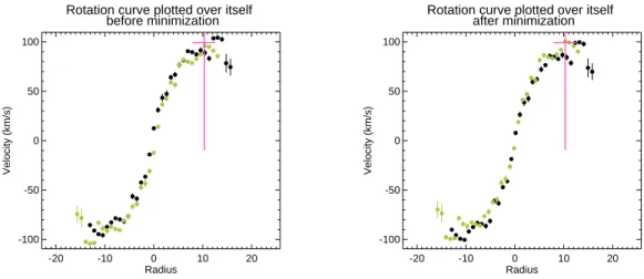
Figure 1. Minimization of the rotation curve of RESOLVE galaxy rf0007. The vertical line is placed at the half-light radius, within which the rotation curve is minimized to find the galaxy’s redshift. The horizontal line shows the galaxy’s Vpmm.
if there are no other good data points within two rows above or below them.
The rotation curve of the major axis slit is next used to measure the asymmetry in the rotation curve, the red-shift which minimizes the asymmetry, and the projected velocity amplitude of the curve (Vpmm). Following the
methods of Raychaudhury et al. (1997), each velocity data point is considered to have a Gaussian distribution with aσ equal to the error on that data point, and the probable maximum velocity is the value which has a 10% likelihood of exceeding all other velocities in the RC. The probable minimum is defined in an analogous way, and Vpmm is defined as half of the difference between the
probable maximum and probable minimum rotation ve-locities.
The code is given an initial guess for the redshift based on the velocity extracted from the spatial center of the continuum, and we use this redshift to determine the rest-frame RC. The asymmetry measurement comes from minimizing the average absolute deviations in velocity between the two halves of the rotation curve as defined by Kannappan et al. (2002) who were extrapolating from a method by Abraham et al. (1996). The asymmetry is recorded as a percentage of the total velocity width 2Vpmm, and is strongly dependent on the spatial and
ve-locity origin of the RC. To recover the best possible value of asymmetry and redshift, we iterate and allow the ori-gin to vary. We constrain the movement of the spatial center by setting a maximum amount,δmax, by which the
spatial origin is allowed to move. This maximum devia-tion,δmax, is first determined by a 3σstandard deviation
from the guess for the spatial center of the continuum. If the 3σ standard deviation is less than 3 pixels, then
δmax is set to 3 pixels because this corresponds to 0.9′′,
the typical seeing of SOAR. If the 3σstandard deviation is greater thanδV pmm/2(defined as the number of pixels
it takes for the curve to rise to Vpmm/2), then δmax is
set to δV pmm/2. The velocity origin is allowed to vary
freely. The minimization and determination of the ori-gin are found using only the inner part of the rotation curve within a radius of Re because of the varying ex-tent of the RCs of the RESOLVE galaxies. Previous work (Courteau 1997; Kannappan et al. 2002) has defined the inner rotation curve to be within 1.3Re because this
rep-resents the peak velocity position for a pure exponential disk (Freeman 1970). We have found, though, that for our current sample of RESOLVE galaxies, the majority of their RCs turn over by Re. The likely reason for this difference is that the Re values found for the RESOLVE galaxies are typically larger than past results due to the fact that we are recovering more light from the galaxy. An example rotation curve before and after minimization is shown in Figure 1.
The spatial point associated with the redshift value de-termined by minimizing the asymmetry is defined to be at the center of the un-collapsed, binned by three im-age of the center slit, and the code now chooses to keep every third point going radially outward from this cen-ter. The extra rows at the ends are discarded, and this becomes the new spectral image. At this point, another round of point rejection occurs to eliminate extracted ve-locities that have no neighboring data points within±2 pixels or that deviate by more than ±400 km s−1 from
the redshift value. We then re-run the asymmetry cal-culation on the final binned, major axis rotation curve for a more robust measurement of the redshift, asym-metry, and Vpmm. The outrigger slits are binned in the
same manner, but the starting point for the binning is the spatial center of the continuum in the spectral im-age. We plan to implement an adaptive binning routine that continues to bin the low signal-to-noise rows until the emission reaches a signal to noise limit of five.
2.4. Kinematically Determined Inclination
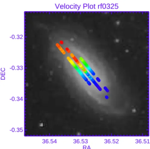
We make use of the rotation curves from all three slits to create velocity fields of the RESOLVE galaxies once the data have been mapped to sky coordinates. We aim to use the velocity fields to fit for kinematic inclinations using the software DiskFit from Spekkens & Sellwood (2007). We have done some preliminary work with this code and have recovered inclinations comparable to our photometric inclinations. This code is dependent on the coordinate information, however, and we are still work-ing on our world coordinate system solution for mappwork-ing velocity points to the correct sky coordinates. An ex-ample velocity field plotted over the SDSS image of the galaxy is shown in Figure 2.
Velocity Plot rf0325
36.54 36.53 36.52 36.51 RA
-0.35 -0.34 -0.33 -0.32
DEC
Figure 2. Velocity field plotted over top of the SDSS image of RESOLVE galaxy rf0325. The rainbow color scale represents the rotation of the galaxy towards (blue points) and away (red points). We do not yet trust the mapping of the velocity points to the sky coordinates.
Another parameter extracted from the spectra using our software is the equivalent width of the Hαemission line, EW(Hα), which is useful as a direct tracer of star formation. The Hαflux calculation is performed in two different ways. The first method is to determine the area under the Gaussian curve that has been fit to the Hα
emission line using the formula for the area under a Gaus-sian. Another approach is to calculate the integrated flux directly from the spectrum by summing all of the data within 3σof the center of the line after subtracting the continuum. The integrated flux is determined in these two ways for each row of the spectral image from which a velocity is measured, along with the continuum flux, and the continuum flux error.
The equivalent width is the integrated flux of the Hα
line divided by the flux of the continuum, and this calcu-lation is performed for all the measurements where the continuum flux is greater than five times the error on the continuum measurement. This precaution is taken be-cause we often measure the Hαflux at large radii in the galaxy where the continuum is very weak. We chose to calculate three different EW(Hα) measurements for each galaxy: the total EW(Hα), the EW(Hα) within 1.3Re, and the EW(Hα) within Re. In the analysis discussed in this thesis, we chose to use the EW(Hα) measurements that were calculated using the flux of Hαas determined by the Gaussian fit because they are more uniformly cal-culated. That is, summing the spectral data within 3σ
of the center of the Hαline sometimes includes data be-yond or inside of the wavelength range of the emission. This may be due to an error in the fit, or perhaps it is due to non-Gaussian emission lines.
3. RESULTS
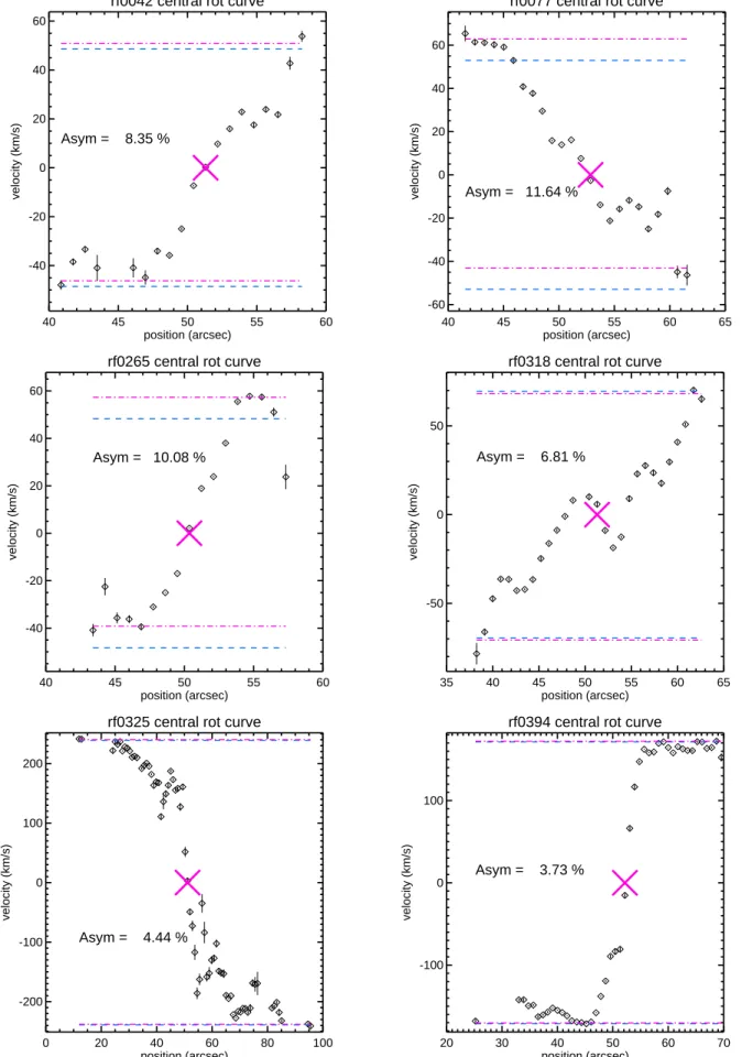
We have extracted rotation curves for 69 galaxies in the RESOLVE survey, but seven galaxies we examined have little to no emission, making it difficult to obtain a reliable measure of their rotation. Of the 62 galaxies with sufficient emission, one of them has outliers in the RC from cosmic rays or high noise peaks that are
skew-ing the Vpmm measurement and making it difficult to
determine a precise redshift, while the initial guess for the redshift of a second galaxy is bad and therefore, we are not obtaining a good Vpmm or redshift. We
there-fore evaluate rotation curves and physical properties ex-tracted from the rotation curves for the other 60 galaxies; six of these are displayed in Figure 3.
We assess the validity of the kinematic information ex-tracted from our rotation curves through comparisons with HI data and results from previous studies. Specif-ically, we compare our redshifts to catalog values, and the distribution of the asymmetries in our sample of 60 RESOLVE galaxies to the distribution of asymmetries in previous work. We compare the Vpmm measurements to
the HI profile linewidths, W50, and verify that our
sam-ple follows the baryonic Tully-Fisher relation (McGaugh et al. 2000). We analyze possible reasons for observed discrepancies between the two measures of rotation veloc-ities by testing dependence of the measurements on other physical parameters extracted from both the optical and HI data. We also present results on the relationship be-tween RC asymmetry and other physical parameters.
3.1. Kinematically Determined Redshift vs. Catalog
Redshift
We compare the redshift as determined by the mini-mization of the asymmetries in the inner portion of the rotation curve to the initial guesses given to the code as described in Section 2.3. Figure 4 shows the difference between the catalog redshift and our redshift vs. our red-shift. The three galaxies whose kinematically determined redshifts are different than the catalog values by ≥100 km s−1 are rf0478, rf0128 and rf0428. For the case of
rf0478, we find that our redshift agrees within the error bars of the SDSS determined redshift, but that both of these are much different from the HyperLEDA redshift. The HyperLEDA redshift is the one that the code de-scribed in Section 2.3 is choosing as the trustworthy red-shift even though it has much larger error bars. Thus, we conclude that this is a mistake and our redshift is not unreasonable for this galaxy. For the cases of rf0128 and rf0428, we find that there is a large difference and we will further investigate our kinematically determined redshift. We further note that it appears that the cata-log redshift is systematically higher at low redshifts, and we are investigating possible causes for this trend. We expect this trend in our data will become more or less ap-parent once we increase our sample size. Excluding the three galaxies that are largely different from the catalog, we find an rms scatter of 35 km s−1. This value is not too
different from the previous findings of 20 km s−1scatter
when comparing various methods for determining central velocity (Keel 1996; Persic & Salucci 1995).
3.2. Distribution of Kinematic Asymmetries
rf0042 central rot curve
40 45 50 55 60
position (arcsec) -40
-20 0 20 40 60
velocity (km/s)
Asym = 8.35 %
rf0077 central rot curve
40 45 50 55 60 65
position (arcsec) -60
-40 -20 0 20 40 60
velocity (km/s) Asym = 11.64 %
rf0265 central rot curve
40 45 50 55 60
position (arcsec) -40
-20 0 20 40 60
velocity (km/s)
Asym = 10.08 %
rf0318 central rot curve
35 40 45 50 55 60 65
position (arcsec) -50
0 50
velocity (km/s)
Asym = 6.81 %
rf0325 central rot curve
0 20 40 60 80 100
position (arcsec) -200
-100 0 100 200
velocity (km/s)
Asym = 4.44 %
rf0394 central rot curve
20 30 40 50 60 70
position (arcsec) -100
0 100
velocity (km/s)
Asym = 3.73 %
4000 4500 5000 5500 6000 6500 7000 Our Redshift (km/s)
-200 -100 0 100 200
Catalog Redshift - Our Redshift (km/s)
Figure 4. Difference between the catalog redshifts and our red-shifts plotted against our redred-shifts.
0 5 10 15
Kinematic Asymmetry (%) 0
2 4 6 8 10
Number of Galaxies
0 5 10 15
Kinematic Asymmetry (%) 0
2 4 6 8 10
Number of Galaxies
Figure 5. Distribution of rotation curve asymmetries for a sample of 60 RESOLVE galaxies.
in which a few dwarf galaxies have kinematic asymme-tries ≥10%. Moreover, Kannappan & Fabricant (2001) look specifically at a sample of 113 NFGS galaxies and find that 26% have asymmetries ≥5%, while our sam-ple shows that 56% have asymmetries ≥5%, and van Eymeren et al. (2011) find 36% of a sample of 70 galax-ies are globally asymmetric. This difference in the overall distribution could be due to the fact that our sample of 60 galaxies are primarily low-mass galaxies that are of-ten more turbulent. It could also be due to differences in spatial resolutions of the data.
3.3. Optical vs. Radio velocity measurements
Kannappan et al. (2002) find that W50and Vpmmagree
very well for the emission-line galaxies in the Nearby Field Galaxy Survey with the following relation found by an iterative least-squares fit with 3.5σ outlier
rejec-tion:
W50[km s−1] = 33(±5)[km s−1]+0.92(±0.02)(2Vpmm)[km s−1]
(1) For our sample of 60 RESOLVE galaxies, the Vpmm and
W50 follow a similar trend, but the relationship is not
as close to a one to one relationship. Figure 6 shows this relationship for both the observed and inclination corrected measurements. The ordinary least-squares for-ward fit lines are plotted in blue for each plot and the fit from Kannappan et al. (2002) is shown in red for com-parison. The fit to our sample of 60 RESOLVE galaxies is as follows:
W50[km s−1] = 50(±17)[km s−1]+0.73(±0.09)(2Vpmm)[km s−1]
(2) The rms scatter in the data relative to this best fit line is 56 km s−1, which is much higher than the 20
km s−1scatter found by Kannappan et al. (2002). The
difference in scatter may be due to the fact that Kannap-pan et al. (2002) exclude certain data points from their fit, such as 3.5σ outliers, galaxies with potentially large P.A. misalignment, and confused HI sources. It is also important to note that they fit the trend to a sample of 96 galaxies compared to our 53.
We also performed an ordinary least-squares fit to inclination-corrected Vpmm and W50that yields:
W50i[km s−
1] = 69(±22)[km s−1]+0.69(±0.1)(2V
pmmi)[km s− 1]
(3) The inclination correction is applied to both the optical and HI velocity measurements by dividing by sin(i). The inclination is defined:
i= cos−1q((b/a)2−q2
0)/(1−q02) (4)
where b/a is the axis ratio and we useq0 = 0.18 as
de-termined by Courteau (1997).
It is sensible that most of the sample of 60 galaxies falls below a rotation velocity of 300km/sbecause RESOLVE is composed of predominantly dwarf galaxies. Figure 7 demonstrates this with a plot of baryonic mass vs. ro-tation velocity. The black Xs are two times the opti-cally determined Vpmm and the red diamonds are the
HI W50 measurements. A Spearman rank test on Vpmm
and baryonic mass yields 100% probability of correlation, while the test on W50and baryonic mass yields a 99.89%
probability. This is an important result as it is consistent with the existence of the baryonic Tully-Fisher relation (McGaugh et al. 2000).
3.4. Kinematic Asymmetry vs. Mass Asymmetry
0 100 200 300 400 500 2Vpmm (km/s)
0 100 200 300 400 500
W
50
(km/s)
0 100 200 300 400 500 600 2Vpmm
i
(km/s) 0
100 200 300 400 500 600
W
50
i (km/s)
Figure 6. Vpmmas determined by the optical rotation curves vs. HI linewidth W50for both the observed (left) and inclination corrected
(right) cases.
1.0 1.5 2.0 2.5 3.0
log[ Vi
(km/s) ] 8
9 10 11 12
log[ Baryonic Mass (Msun) ]
Figure 7. Baryonic mass (MSun) vs. inclination corrected
rota-tion velocity (km/s). The X’s are two times Vpmm and the red
diamonds are HI W50measurements.
We compare mass asymmetries to optical RC kine-matic asymmetries for 49 of our 60 RESOLVE galax-ies. There are 49 to compare because only 53 of the 60 galaxies have HI detections, and four of these galax-ies have unreliable HI asymmetry measurements due to extremely low signal-to-noise, a bad HI baseline, or the HI redshift being drastically different from the optical redshift and all other catalog redshifts. As shown in Fig-ure 8, there is no clear correlation between the kinematic and mass asymmetries. For example, there are several galaxies which show a very high asymmetry in the HI profile, while the asymmetry in the rotation curve is rel-atively small. This implies an asymmetric distribution of HI gas where the motions of the ionized gas are relatively more symmetric.
There have been differing results from previous com-parisons of this type. Swaters (1999) reports on a
spe-0 5 10 15 20
Kinematic Asymmetry (%) 0
20 40 60 80 100
Mass asymmetry (%)
Figure 8. HI profile asymmetry vs. optical rotation curve asym-metry.
cific dwarf galaxy, NGC 4395, that shows kinematic asymmetries but no asymmetry in HI. On the contrary, Jog (2002) argues that the two measurements should be correlated, specifically for spiral galaxies, because they should be coupled via the continuity equation for par-ticles on perturbed orbits in a lopsided disk potential defined in Jog (1997).
3.5. Asymmetry as a reason for velocity discrepancies
We examine the relationship between asymmetries and rotation velocities for all combinations of the HI pro-file (mass) asymmetry, HαRC (kinematic) asymmetry, Vpmm, and W50. The strongest correlation exists
be-tween the kinematic asymmetry and Vpmm; a Spearman
rank test on this relation produces a correlation proba-bility of 99.5%. There is a 2σcorrelation between mass asymmetry and W50 with a correlation probability of
kine-matic asymmetry and W50, or between mass asymmetry
and Vpmm.
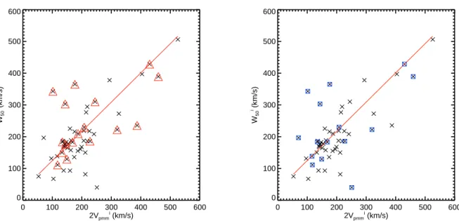
To test whether asymmetries are causing a discrep-ancy between Vpmmand W50, we examine the placement
of galaxies with the highest asymmetries in Figure 9. We identify galaxies with kinematic asymmetries greater than or equal to 10% (left) and the placement of galaxies with HI mass asymmetries greater than or equal to 60% (right) because we consider these percentages and above to be anomalous. It appears that the kinematic asymme-tries are not responsible for the major discrepancies, as those with high asymmetry fall relatively close to the fit line. In the case of mass asymmetry, however, it appears that for some galaxies this may be a significant source of discrepancy in the velocity measurements.
3.6. HI source confusion as a reason for velocity
discrepancies
We examine the velocity placement of galaxies that have been flagged as confused HI sources, and galaxies with neighbors within 0.1 Mpc because these galaxies could be potentially undergoing an interaction that is causing a velocity discrepancy. These plots are shown in Figure 11 with the confused galaxies overlaid on the left and those with a close neighbor overlaid on the right.
The HI confused flag comes from the fact that the radio telescope beam is very large and there is often more than one HI source in the beam when attempting to observe a particular galaxy. The confusion flag is automated and does not mean that the HI profile is definitely blended with that of another HI source. For example, Figure 10 shows the HI spectrum from ALFALFA for RESOLVE galaxy rf0011; this galaxy is not obviously confused with another source, but it was flagged as such. Nonetheless, it is interesting that the three galaxies that lie farthest above the best fit line are all flagged as confused. That is, the fact that these are flagged as confused sources is consistent with the fact that these galaxies have HI linewidths that are much wider than the velocity pro-file as measured from the optical rotation curves. This could imply that the Vpmm is a better measure of these
galaxies’ rotation velocities.
3.7. Close neighbors as a reason for velocity
discrepancies
Similarly, the discrepancy between W50and Vpmm for
galaxies with neighbors within 0.1 Mpc provides some interesting insight. Figure 11 shows that the galaxies that fall farthest from the best fit line often also have close companions. We examine the relationship between velocity discrepancy and distance to nearest neighbor in Figure 12. Although there is no linear correlation in the plot of the difference between W50 and Vpmm vs.
distance to the nearest neighbor, it is clear that galaxies with large discrepancies in velocity have a close neighbor. Distance to nearest neighbor could be related to sev-eral reasons for discrepancies between the two velocity measurements. One possibility is that the close neighbor is causing HI source confusion as discussed in 3.6. Fur-thermore, an interaction with this neighbor could lead to inconsistencies between the motions of the ionized and neutral gas because it could be disrupting the bulk
flow of one or both types of gas. The interaction could tidally disrupt ionized gas and/or neutral gas to one side of the galaxy causing kinematic and/or mass asymme-tries. Asymmetries may also result from violent encoun-ters that decouple the gas from the stellar continuum peak (Barton et al. 2001; Mihos 2001). We further dis-cuss the correlation between kinematic asymmetry and nearest neighbor distance in Section 3.10.5. Another pos-sibility is that the interaction is causing gas inflow, thus truncating the rotation curve or narrowing the HI pro-file linewidth (Hernquist & Mihos 1995; Barton Gillespie et al. 2003). However, a plot of rotation curve extent vs. nearest neighbor distance reveals that there is no corre-lation whatsoever between these parameters.
We note that there are galaxies that have a very close neighbor, but a small difference between W50and Vpmm.
This result does not necessarily contradict the idea that interactions are a cause for discrepancy, however, because the disturbance of the gas is heavily dependent upon the location of the two galaxies relative to one another and the state of their interaction (Woods et al. 2006). Fur-thermore, the effects of interactions may manifest them-selves in the galaxy morphology, or gas or stellar dy-namics, depending on the strength of the interaction and the environment in which the galaxy resides (Marquez & Moles 1996; Dale et al. 2001). Thus, assessing only the gas dynamics is not a conclusive method for determining if an interaction is taking place.
3.8. RC truncation as a reason for velocity
discrepancies
Figure 13 shows that there may also be significant dis-crepancies for galaxies with truncated rotation curves. This parameter should be considered with caution be-cause we have not yet implemented binning that allows us to reach particularly low signal-to-noise Hαemission. Thus, it may be that the ionized gas extends farther than our velocity extraction indicates. Figure 13 is also dif-ferent from the results of Kannappan et al. (2002), who found that truncated RCs show no strong deviation from the W50 vs. Vpmm correlation.
3.9. Low HI peak signal-to-noise as a reason for velocity
discrepancies
There does not appear to be a relationship between the discrepancies between Vpmm and W50 and the peak
signal-to-noise ratio of the HI data. This fact is demon-strated in Figure 13 where we have indicated the galaxies with a peak signal-to-noise of less 5.
3.10. Further exploration of RC Asymmetry
Here, we explore other physical parameters for causes of kinematic asymmetries. We find some hints of corre-lations but no statistically significant results.
3.10.1. Asymmetry and Inclination
0 100 200 300 400 500 600 2Vpmm
i
(km/s) 0
100 200 300 400 500 600
W
50
i (km/s)
0 100 200 300 400 500 600 2Vpmm
i
(km/s) 0
100 200 300 400 500 600
W
50
i (km/s)
Figure 9. Galaxies with kinematic asymmetries≥10% (left) and mass asymmetries ≥60% (right) as they fall on the W50 vs. Vpmm
relationship
Figure 10. HI spectrum from the ALFALFA survey for RESOLVE galaxy rf0011. This galaxy was automatically flagged as a confused HI source, though it is not obvious from looking at its spectrum that it is confused.
have inclinations smaller than 40◦. Figure 14 shows that there is not a significant trend between optical RC asym-metry and inclination, particularly above the threshold of 40◦. A Kolmogorov-Smirnov test finds that there is a 94% chance that the trend in asymmetry with inclina-tion below 40◦ is different from that above 40◦. Thus, the determined asymmetries of galaxies with inclinations above 40◦ are likely mainly due to kinematic anomalies within the galaxy, but below this threshold the asymme-tries may be due to higher turbulence in relation to the velocity that we measure.
3.10.2. Asymmetry and Extent
Consistent with the results of Kannappan & Barton (2004), we find no significant correlation between kine-matic asymmetries and extent of the rotation curve. That is, there are very few galaxies with both a trun-cated rotation curve and large kinematic asymmetry as shown in Figure 15.
3.10.3. Star formation and Asymmetry
0 100 200 300 400 500 600 2Vpmm
i
(km/s) 0
100 200 300 400 500 600
W
50
i (km/s)
0 100 200 300 400 500 600
2Vpmm i
(km/s) 0
100 200 300 400 500 600
W
50
i (km/s)
Figure 11. Galaxies flagged as confused HI sources (red triangles on the left) and with neighbors within 0.1 Mpc (blue squares on the right) as they fall on the W50vs. Vpmm relationship.
0.0 0.5 1.0 1.5 2.0 2.5
Distance to Nearest Neighbor (Mpc) 0
50 100 150 200 250
abs[ W
50
i - V
pmm
i (km/s) ]
Figure 12. W50- Vpmm(km/s) vs. distance to nearest neighbor
(Mpc).
Spearman rank test shows a very weak (2σ) correlation between kinematic asymmetries and the long-term frac-tional stellar mass growth rate, FSMGR, measuring star formation rate over the past Gyr as defined by Kannap-pan et al. (2013). We investigate the possibility that this 2σ correlation is a result of both kinematic asymmetry and FSMGR correlating with a third parameter such as baryonic mass or absolute magnitude. There is a 3σ cor-relation between FSMGR and both baryonic mass and absolute magnitude, but kinematic asymmetry shows no correlation with either of these. We do find that there is a strong correlation between kinematic asymmetry and Vpmm and between FSMGR and Vpmm yielding percent
correlations of 99.5% and 99.9%, respectively. This result is a purely empirical because Vpmm in this relationship
has not been corrected for inclination, which explains the lack of correlation between kinematic asymmetry and baryonic mass despite the correlation between Vi
pmmand
baryonic mass.
3.10.4. Asymmetry and color
There is no clear trend between kinematic asymmetries and u-r color, though the majority of galaxies with kine-matic asymmetries ≥ 7% are very blue as one can see in Figure 16. There are two exceptions to this, galaxies rf0233 and rs0733, which are very red in color, but have kinematic asymmetries greater than 10%. Upon observ-ing the rotation curves of these two galaxies, as well as inspecting the data points that were extracted from the spectra, it is evident that this value of total asymmetry is trustworthy for galaxy rf0233, but should be re-assessed for galaxy rs0733. In the case of rf0233, the galaxy ap-pears to be very rapidly rotating with a lot of turbulence.
3.10.5. Asymmetry and Nearest Neighbor Distance
There is no linear correlation between kinematic asym-metries and distance to the nearest neighbor, but all of the galaxies with asymmetries greater than 10% have neighboring galaxies within 0.6 Mpc. It is also observed that there is no linear correlation between mass asymme-try and distance to the nearest neighbor, but the major-ity of galaxies with a mass asymmetry greater than 40% have a neighbor within 0.6 Mpc. These relationships are shown in Figure 17.
4. DISCUSSION
We have successfully developed software for extracting galaxy rotation curves from 2D RESOLVE spectra. This software has been added to the end of our data reduction pipeline to be used on all RESOLVE galaxies that have been observed in the setup described in Section 2. The kinematic information obtained from this software will be useful to the scientific goals of the RESOLVE survey in many ways. In particular, Vpmmmeasurements will be
0 100 200 300 400 500 600 2Vpmm
i
(km/s) 0
100 200 300 400 500 600
W
50
i (km/s)
0 100 200 300 400 500 600
2Vpmm i
(km/s) 0
100 200 300 400 500 600
W
50
i (km/s)
Figure 13. Galaxies with truncated rotation curves (blue asterisks on the left) and HI peak signal-to-noise of less than 5 (pink diamonds on the right) as they fall on the W50vs. Vpmmrelationship.
0 5 10 15 20
Kinematic Asymmetry (%) 0
20 40 60 80 100
inclination (degrees)
Figure 14. Inclination vs. Optical rotation curve asymmetry.
of velocities for galaxies in all environments (Kannappan & RESOLVE Team 2013). Furthermore, Hα equivalent widths, kinematic asymmetries, the extent of the rota-tion curves, and measures of turbulence in the rotarota-tion curves can all be used for probing star formation and merger activity within the RESOLVE galaxies.
This thesis work has focused specifically on check-ing the quality of the RESOLVE velocity measurements through comparison of the optically determined Vpmm
and the HI profile linewidth at 50%, W50, as determined
from the radio data. Identifying reasons for any discrep-ancies between these measurements is important for de-ciding which is a better quality measurement to be used for further calculations, such as the dynamical mass.
We have tested several reasons for these discrepan-cies and found that a galaxy-galaxy interaction is a likely mechanism for large differences as indicated in Fig-ures??. Figures 9 and 13 indicate that large mass asym-metries and truncated rotation curves are also drivers of
0.5 1.0 1.5 2.0 2.5 3.0
RC Extent (Re) 0
5 10 15 20
Kinematic Asymmetry (%)
Figure 15. Kinematic asymmetry vs. extent of rotation curve as a function of Re for a sample of 60 RESOLVE galaxies.
these differences, but it is possible that the mass asym-metries and truncations are both induced by the interac-tions. That is, an interaction may pull the gas to one side of the galaxy causing a large mass asymmetry (Marquez & Moles 1996; Dale et al. 2001), or the interaction could cause a gas inflow resulting in RC truncation (Hernquist & Mihos 1995; Barton Gillespie et al. 2003).
0 5 10 15 20 Kinematic Asymmetry (%)
0.0 0.5 1.0 1.5 2.0 2.5
u-r
Figure 16. Kinematic asymmetry vs. u-r color. The vertical line is positioned at an asymmetry of 7% to help see that the majority of galaxies with asymmetries greater than this threshold are blue.
In an attempt to identify which gas component - neu-tral or ionized - is more affected by the close neighboring galaxy, we have revisited the baryonic Tully-Fisher rela-tion for galaxies with a neighbor within 0.3 Mpc for both Vi
pmm and Wi50. Figure 18 shows these relationships. A
Spearman rank test on both plots reveals that there is still a strong, 3σcorrelation between Vpmmand baryonic
mass, while the correlation between W50 and baryonic
mass has dropped to a probability of 96.1%. This result implies that the neutral gas W50 is more affected by a
neighboring galaxy than the optical Vpmm.
5. CONCLUSIONS AND FUTURE WORK
We conclude that our rotation curve extraction soft-ware is effective and produces reliable results. We are confident in both the Vpmm and kinematic asymmetry
measurements produced from this software. We are con-fident in approximately half of the redshifts determined from minimizing the asymmetries in the inner radii of the rotation curve, and we are further investigating dis-crepancies between our redshift and the catalog redshifts. We believe that analyzing a larger sample of RESOLVE galaxies will illuminate any necessity for modifying our code for determining redshifts.
We plan to improve our software through the imple-mentation of an adaptive binning code that will con-tinue to sum rows of the spectral image until a signal to noise of 5 is reached, allowing us to probe low signal to noise Hαemission. Extracting velocity measurements from low signal to noise emission will improve our Vpmm,
kinematic asymmetry, and redshift calculations. We also hope that we will better quantify the spatial extent of the ionized gas within the galaxy.
Furthermore, once we have resolved the problems with our world coordinate system solution and are properly mapping our velocities to sky coordinates, we will pro-duce velocity fields that enable us to fit for the kinematic inclination of the galaxy. With this information, we can determine the rest-frame velocities of the RESOLVE galaxies and perform dynamical mass calculations. We can then calculate dark matter masses by subtracting the
baryonic mass from the dynamical mass.
We have investigated reasons for discrepancies between Vpmm and W50 and identified galaxy interactions as a
likely mechanism for the observed differences. It may be that an interaction is causing either the ionized or neutral gas to reflect a rotation velocity that is either larger or smaller than the actual bulk rotation of the matter within the galaxy. It may be that an interaction is tidally disrupting either one or both types of gas, re-sulting in mass and/or kinematic asymmetries (Barton et al. 2001; Mihos 2001), or it may be that the interac-tion is forcing an inflow of gas toward the galaxy center. The latter could cause a narrow HI profile linewidth or truncation of the optical RC (Hernquist & Mihos 1995; Barton Gillespie et al. 2003).
Finally, we have shown using the baryonic Tully-Fisher relation that Vpmm is a more robust measurement than
HI W50 for galaxies with a galaxy neighbor within 0.3
Mpc. This result could have major implications for the global distribution of internal velocities of galaxies and galaxy clusters or the “velocity function”. Measuring this distribution is one of the major goals of the RE-SOLVE survey as it is an observable proxy for the halo mass function (Kannappan & RESOLVE Team 2013). Previously, this measurement has been probed using HI data (Papastergis et al. 2013). RESOLVE will improve this study of the velocity function given that these pre-liminary results imply that Vpmm yields a more robust
measurement than HI W50.
Mex-0 5 10 15 20 Kinematic Asymmetry (%)
0.0 0.5 1.0 1.5 2.0 2.5
Distance to Nearest Neighbor (Mpc)
0 20 40 60 80 100
Mass Asymmetry(%) 0.0
0.5 1.0 1.5 2.0 2.5
Distance to Nearest Neighbor (Mpc)
Figure 17. Kinematic asymmetry (left) and mass asymmetry (right) vs. Nearest Neighbor Distance.
1.6 1.8 2.0 2.2 2.4 2.6 2.8 log[ 2Vpmm
i
(km/s) ] 7
8 9 10 11 12 13
log [ Baryonic Mass (Msun) ]
1.4 1.6 1.8 2.0 2.2 2.4 2.6 2.8 log[ W50
i
(km/s) ] 7
8 9 10 11 12 13
log [ Baronic Mass (Msun) ]
Figure 18. Baryonic Tully-Fisher relation using Vpmm (left) and W50 (right) for galaxies with nearest neighbors within 0.3 Mpc. This
plot shows that for this sample of galaxies, baryonic mass retains a strong correlation with Vpmm but it only has a 96.1% probability of
correlating with W50.
ico State University, New York University, Ohio State University, Pennsylvania State University, University of Portsmouth, Princeton University, the Spanish Partici-pation Group, University of Tokyo, University of Utah, Vanderbilt University, University of Virginia, University of Washington, and Yale University. We acknowledge the use of the HyperLEDA and ALFALFA databases. We acknowledge the use of Arecibo data. The Arecibo Observatory is the principal facility of the National As-tronomy and Ionosphere Center, which is operated by the Cornell University under a cooperative agreement with the National Science Foundation.
REFERENCES
Abraham, R. G., Tanvir, N. R., Santiago, B. X., et al. 1996, MNRAS, 279, L47
Acker, A. 1989, in IAU Symposium, Vol. 131, Planetary Nebulae, ed. S. Torres-Peimbert, 39–48
Barton, E. J., Geller, M. J., Bromley, B. C., van Zee, L., & Kenyon, S. J. 2001, AJ, 121, 625
Barton Gillespie, E., Geller, M. J., & Kenyon, S. J. 2003, ApJ, 582, 668
Beauvais, C., & Bothun, G. 2000, ApJS, 128, 405
Clemens, J. C., Crain, J. A., & Anderson, R. 2004, in Society of Photo-Optical Instrumentation Engineers (SPIE) Conference Series, Vol. 5492, Ground-based Instrumentation for Astronomy, ed. A. F. M. Moorwood & M. Iye, 331–340 Courteau, S. 1997, AJ, 114, 2402
Dale, D. A., Giovanelli, R., Haynes, M. P., Hardy, E., & Campusano, L. E. 2001, AJ, 121, 1886
Freeman, K. C. 1970, ApJ, 160, 811
Giovanelli, R., Haynes, M. P., Kent, B. R., et al. 2005, AJ, 130, 2598
Haynes, M. P., van Zee, L., Hogg, D. E., Roberts, M. S., & Maddalena, R. J. 1998, AJ, 115, 62
Jog, C. J. 1997, ApJ, 488, 642 —. 2002, A&A, 391, 471
Kannappan, S., & RESOLVE Team. 2013, in Probes of Dark Matter on Galaxy Scales, 10203
Kannappan, S. J., & Barton, E. J. 2004, AJ, 127, 2694 Kannappan, S. J., & Fabricant, D. G. 2001, in Astronomical
Society of the Pacific Conference Series, Vol. 230, Galaxy Disks and Disk Galaxies, ed. J. G. Funes & E. M. Corsini, 449–450 Kannappan, S. J., Fabricant, D. G., & Franx, M. 2002, AJ, 123,
2358
Kannappan, S. J., & Wei, L. H. 2008, in American Institute of Physics Conference Series, Vol. 1035, The Evolution of Galaxies Through the Neutral Hydrogen Window, ed. R. Minchin & E. Momjian, 163–168
Kannappan, S. J., Stark, D. V., Eckert, K. D., et al. 2013, ApJ, 777, 42
Keel, W. C. 1996, ApJS, 106, 27
Marquez, I., & Moles, M. 1996, A&AS, 120, 1
McGaugh, S. S., Schombert, J. M., Bothun, G. D., & de Blok, W. J. G. 2000, ApJ, 533, L99
Mihos, J. C. 2001, ApJ, 550, 94
Papastergis, E., Giovanelli, R., Haynes, M. P., Rodr´ıguez-Puebla, A., & Jones, M. G. 2013, ApJ, 776, 43
Paturel, G., Petit, C., Prugniel, P., et al. 2003, A&A, 412, 45 Persic, M., & Salucci, P. 1995, ApJS, 99, 501
Persic, M., Salucci, P., & Stel, F. 1996, MNRAS, 281, 27 Raychaudhury, S., von Braun, K., Bernstein, G. M., &
Guhathakurta, P. 1997, AJ, 113, 2046
Richter, O.-G., & Sancisi, R. 1994, A&A, 290, L9 Spekkens, K., & Sellwood, J. A. 2007, ApJ, 664, 204
Swaters, R. A. 1999, PhD thesis, , Rijksuniversiteit Groningen, (1999)
Tully, R. B., & Fisher, J. R. 1977, A&A, 54, 661 van Dokkum, P. G. 2001, PASP, 113, 1420
van Eymeren, J., J¨utte, E., Jog, C. J., Stein, Y., & Dettmar, R.-J. 2011, A&A, 530, A29
Woods, D. F., Geller, M. J., & Barton, E. J. 2006, AJ, 132, 197 York, D. G., Adelman, J., Anderson, Jr., J. E., et al. 2000, AJ,