C
OMPACT
: A Rational Expectations, Intertemporal
Model of the United Kingdom Economy
Julia Darby
a, Jonathan Ireland
b, Campbell Leith
c, Simon Wren-Lewis
ca Department of Economics, University of Glasgow, Glasgow G12 8RT
b Department of Economics, University of Strathclyde, Glasgow G4 0LN
c Department of Economics, University of Exeter, Exeter EX4 4RJ
Abstract
COMPACT is a quarterly macro econometric model of the UK primarily designed for
policy analysis. The model includes a consumption function derived explicitly from intertemporal optimisation, a vintage production technology, nominal rigidities in wage and price setting, and trade equations which are influenced by the variety and quality of production relative to the rest of the world. We discuss the overall properties of the model, as well as features of major equations. We stress the importance of relating these properties to simpler theoretical paradigms. Several
simulations illustrating key properties of COMPACT are presented. A complete
equation listing is provided in an Appendix.
JEL Classification E1 E60 C51 C52
Keywords United Kingdom; Econometric model; Consumption; NAIRU; Vintage production.
Acknowledgements
Development of COMPACT would not have been possible without financial support
from the UK Economic and Social Research Council’s Macro-Economic Modelling Consortium under grants W116251011 and L116251026, and initial development support from the University of Strathclyde. The model presented here owes a great deal to the work of other colleagues, including Ottavio Ricchi, Rebecca Driver, Paul Warren, Carole Owen and Paul Ashworth. We are grateful to Andrew Stevenson for his helpful comments on an earlier version of this paper.
1. Introduction
This paper provides a detailed account of the quarterly UK econometric
model COMPACT. The first version of the model was completed in 1993 at the
University of Strathclyde, about a year and a half after work began. We describe here version 3.0 of the model which was completed in late 1996, although the overall structure of the model has not altered significantly since the first version was
finished.1 COMPACT is not attached to any particular institution, but instead represents
the efforts of a number of individuals working in the UK academic sector.
A central aim of COMPACT is to apply modern macroeconomic theory to
UK data in a form which can contribute to the macroeconomic policy debate. Our focus is on policy analysis rather than short term forecasting and we do not use COMPACT as a forecasting tool. (See Wren-Lewis, 1993A, for a discussion of the
potential conflicts between model development and forecasting.) We stress the importance of being able to relate model properties to simpler theoretical paradigms
(see Wren-Lewis et al, 1996), without sacrificing the generality and versatility of a
complete model with firm links to historical data. These considerations were crucial in
determining the size of COMPACT, which derives its name from the fact that it is rather
smaller than many other UK econometric models.
The structure of the paper is as follows. Section 2 discusses the theoretical properties of the model as a whole, as well as features of its key equations. Section 3 presents some full model simulations, most of which have not been presented
elsewhere. Section 4 briefly outlines future development plans for COMPACT, and
draws on the experience of building and using this model to make some general observations on the role of econometric macroeconomic models. An Appendix
provides a complete equation listing of COMPACT 3.0.
COMPACT is solved using its own software, which was written using Borland’s
DELPHI program for use in Windows 3.1 or Windows 95/NT. The model and software
are available on request for anyone wishing to use COMPACT for academic purposes.2
2. Theoretical Structure
1 In common with the other ESRC supported macroeconomic models, COMPACT is deposited at the
ESRC Macroeconomic Modelling Bureau at Warwick University. In Church et al, 1997, the Bureau compares the properties of COMPACT 3. 0 with other UK models.
2 Contact Simon Wren-Lewis on [email protected] or alternatively visit our web page at
The two main sets of agents in the model are consumers and firms. Consumers maximise utility subject to an intertemporal budget constraint, although their ability to borrow on future income may additionally be constrained by the behaviour of lending institutions. Firms maximise discounted profits subject to a vintage production technology and various convex adjustment costs. Where agents form expectations, these are typically assumed to be “rational” or, more formally, model consistent.
Goods and labour markets are imperfectly competitive. In particular wages are set as a result of bargaining between unions and firms although, in common with most of the empirical literature in this area, there is no formal link between union and consumer/worker preferences. The demand curve for goods is reflected in the model's trade equations. Here an important innovation is to endogenise non-price competition (through increased quality or variety) by linking it to past levels of investment.
In analysing the properties of the model, it is useful to divide the time frame
into the short (1-4 years), medium (5-30 years) and long run.3
2.1 The Short Run
In the short run nominal inertia in price and wage setting gives rise to Keynesian type effects on output. Indeed the combination of nominal inertia and rational expectations in wage and price setting allow the model to be described as New
Keynesian. Nominal inertia arises from only two sources in COMPACT: staggered
annual contracts in wage setting (see Moghadam and Wren-Lewis, 1994, and the description of the wage W equation in Appendix II), and ‘quadratic’ adjustment costs in aggregate prices (see the description of the equation for the price of non-oil output PYNO in Appendix II). The price and wage equations can be combined to form an equation similar to an expectations augmented Phillips curve which includes forward looking terms in the pressure of demand in the labour and good markets (Ireland and Wren-Lewis, 1998, provides further details).
The existence of nominal inertia implies that output in the short run will depend on effective demand. The short run behaviour of demand reflects the behaviour of its components. Many features, such as stock adjustment, import leakages and the investment accelerator are familiar in macroeconometric models.
Important effects in COMPACT 3.0 which influence effective demand and which may
3 COMPACT’s vintage production technology results in a slower adjustment to the long run than in
be less familiar are jumps in the exchange rate and consumption generated by forward looking behaviour.
The nominal exchange rate is determined by a forward looking uncovered interest parity condition. Any change in interest rates will therefore be reflected in a change in the path of the exchange rate with, for example, a rise in UK interest rates producing a compensating depreciation over the period of the interest differential. In the case where interest rates are constant throughout a simulation, the profile of the nominal exchange rate over time will be flat with the entire profile adjusting in a direction which achieves long run stability in the net overseas assets to GDP ratio, i.e. an asset stock equilibrium. Thus in any simulation which would otherwise have led to a long run change in the current account, the exchange rate will jump in a compensating direction. This means that with constant interest rates any changes in the real exchange rate beyond that caused by the initial jump in the nominal rate must be generated through changes in prices alone. The combination of nominal inertia in
price and wage setting and this behaviour of the exchange rate means that COMPACT
shares a number of characteristics of the Dornbusch, 1976, ‘overshooting’ model with initial jumps in the exchange rate which overshoot the long run value.
Jumps in the level of consumption typically occur for two reasons, either because consumers’ discounted lifetime labour income is expected to change, or because changes in real interest rates lead to a new optimal distribution of
consumption over time. The basic consumption function in COMPACT is consistent
with a forward looking Blanchard-Yaari model where utility is logarithmic and future labour income is discounted at a constant mark up on the real interest rate. This gives an aggregate function for those consumers who do not face a binding credit constraint
Cf Hf Af
where H is human wealth or discounted lifetime labour income, A is real net financial
and physical wealth and is a constant parameter. In addition, COMPACT’s
consumption function also allows for a variable proportion of income going to consumers who are not able to borrow as much as they would like against their future
income and who consequently spend all their available income.4 The principal
determinant of the proportion of labour income received by credit constrained consumers is an exogenous measure of the degree of financial liberalisation through
the 1980s constructed by Muellbauer and Murphy, 1991. Details of the estimated equation for consumption, CP, are given in Appendix II.
A rise in real interest rates in COMPACT will lead, ceteris paribus, to a jump
down in consumption followed by a more rapid growth rate. This is best explained by reference to a Keynes-Ramsey optimality rule which links the growth rate of the forward looking element of consumption to the real interest rate (see Blanchard and Fischer, 1989, chapters 2 & 3). In particular, a rise in the real interest rate leads to a corresponding increase in the growth rate of consumption which, given the steady
state relationship between consumption and personal sector net wealth A5, can only be
accommodated by a downwards jump in current consumption.
Traditional mechanisms behind the Keynesian multiplier are relatively weak in COMPACT for temporary changes in income. Forward looking consumers will smooth
any short term change in income resulting in only modest changes in consumption. On the other hand, those consumers who face binding credit constraints will respond fully and immediately to any income change, but this effect is weak since the credit constrained group are estimated to have contributed only a relatively small proportion
of total consumption in recent years 6.
Multiplier type effects can, however, arise through the powerful influence of real interest rates upon aggregate demand. An increase in demand will result in inflationary pressure which, given any inertia in the response of nominal interest rates to inflation, will reduce real rates. As we have seen above, lower real interest rates will then result in a positive jump in current consumption. In addition lower real rates will induce an upward jump in investment. These changes in demand are reinforced by accelerator effects, which occur in both investment and stockbuilding.
In practice, the response of nominal interest rates to inflation depends critically
upon the chosen monetary policy rule, which in COMPACT is expressed through the
equation for short term interest rates RS. Many simulations in COMPACT can in fact be
run under the assumption of constant nominal interest rates. The Sargent and Wallace, 1975, result that fixed nominal interest rates are destabilising only applies to simple
models that exclude wealth effects and nominal debt. COMPACT will normally solve
without any problem under fixed nominal rates, as will simple forward looking theoretical models that include nominal government debt (see Leith, Warren and Wren-Lewis, 1997).
5 The steady state properties of COMPACT are discussed in more detail in Wren-Lewis et al (1996). 6 Specifically, 20% of labour income is currently estimated to go to credit constrained consumers and
However, for simulations involving permanent changes, a constant nominal interest rate rule can generate large movements in the long run price level, and corresponding large initial jumps in the nominal and (given price inertia) real exchange rates. The model’s interest rate reaction function allows the level of real interest rates to respond to differences between actual and target inflation, and
deviations from base in the price level.7 In COMPACT 3.0 this rule is routinely used for
simulations involving permanent changes. However for temporary shocks we have found that using this rule tends to increase rather than reduce short run inflation, for reasons described in Leith and Wren-Lewis, 1997. The model’s interest rate, RS, reaction function is set up in a flexible fashion so that the user can change the form of the policy rule, although care needs to be exercised as it is quite easy to choose rules that generate model instability.
Excess demand influences inflation through two main routes. First, changes in unemployment influence wages through wage bargaining between firms and unions. Lower unemployment will raise the target wage WSTAR to which actual wages W adjust towards through staggered annual contracts. Second, costs do depend upon
capacity utilisation through COMPACT’s vintage production function. In the short run,
an increase in output will be met by firms using older, less efficient machines, before any new investment comes on stream. As these older less efficient machines are producing marginal output, marginal costs will rise and put upward pressure on
prices.8 The mark up of prices over costs is independent of demand.
2.2 The Medium Run
In the medium run, the level of unemployment tends to the NAIRU or natural rate of unemployment. This convergence occurs in part through trade effects: with the nominal exchange rate on its open arbitrage path, changes in domestic inflation lead to changes in competitiveness which alter the demand for domestic production. Changes in inflation also generate changes in the real value of government debt, which influences consumption. The NAIRU is reached when the real wage set by firms in the goods market (as a mark-up over costs) is equal to the real wage set by bargaining in
the labour market (see Layard et al, 1991, for example).
7 The operation of rules of this type is analysed in Leith and Wren-Lewis, 1996, and more generally
in Taylor, 1993.
8 Prices PYNO adjust towards a target price PSTAR which is given by a constant mark up on a
weighted average of marginal and average costs. See the description of the vintage model in Appendix I and the equation listings for PSTAR and PYNO in Appendix II.
In COMPACT, the NAIRU is independent of tax wedges and benefits, but it
does depend on the extent of trade union coverage. The most important endogenous determinant of the NAIRU in the model is the relationship between average levels of labour productivity (which influences the bargained real wage), and productivity on the marginal machine used in production (because marginal costs help determine
prices). In a standard Layard et al, 1991, model with a Cobb-Douglas putty-putty
production function the ratio of marginal to average productivity is constant.
However, in COMPACT the ratio varies in the short and medium term due to the
vintage structure of production even though the ex ante production function is Cobb-Douglas; see Appendix I for further details.
A period of rapid investment will tend to reduce the age of the oldest machine in use, and since technical progress is embodied in machines this will raise marginal productivity by more than average productivity. Marginal costs will fall and the real wage (sometimes known as the price determined real wage) consistent with price setting behaviour increases. Rising average productivity means that the bargained real wage increases too, but given that marginal productivity increases by more than average productivity, the movement in the price determined real wage dominates and the NAIRU will tend to fall over the medium run.
As investment tends to rise after any demand shock, this medium run fall in the NAIRU gives the model a hysteresis property which is similar to endogenous growth effects. Unlike endogenous growth, however, this investment effect is not permanent. This is because subsequent investment responds to the productivity differential between the oldest, marginal machine and new machines (see the equation for non-oil investment INO in Appendix II for more details). As the marginal machine becomes more productive, the investment to output ratio will fall slightly, which raises the age
of the marginal machine and reduces its productivity.9
The supply side effects of investment are crucial in determining the medium
term properties of the model in a second way. In COMPACT both exports and imports
are influenced by the variety and quality of UK production relative to the rest of the
world10, which we proxy by cumulated past investment levels. A period of strong
investment growth gradually increases the demand for UK production. If the NAIRU falls, the increase in demand will raise UK output, but to the extent that the increase in
9 The influence of a vintage production technology upon the NAIRU is discussed in detail in Darby,
Ireland and Wren-Lewis, 1995.
10 This follows international trade models based upon imperfect competition such as those in
supply exceeds or falls short of the extra demand for UK output then some other variable (such as the real exchange rate) has to adjust.
Both these medium term properties of COMPACT are ‘non-standard’, in the
sense that they are not part of the core of mainstream theoretical macroeconomics. As
most of the rest of COMPACT is standard in this sense, it is important to be able to
distinguish between features of model simulations that are due to these non-standard elements and those that are not. Wren-Lewis et al, 1996, describes how to use the technique of ‘theoretical deconstruction’ to do this, using the two effects outlined above as illustrations. (See Section 3 below for a brief explanation of this technique.)
A more standard influence upon medium term properties arises from the
behaviour of fiscal policy. COMPACT 3.0 includes a feedback rule for income tax
which changes personal income taxes if the government debt to GDP ratio diverges from its base value. In practice this makes the steady state debt to GDP ratio a
function of the ratio of government spending to GDP.11 More precisely, if the
government spending to GDP ratio does not change in a simulation the rule ensures that the ratio of government debt to GDP stabilises at its base level in the long run. This feedback rule is preferable to an alternative assumption of constant tax rates, because under constant rates any positive shock to government debt would result in a steady but explosive build up of government debt interest payments or possibly in inflation stimulated by an initial expansion in demand which would erode the real value of debt. It is important to note that this simple fiscal feedback rule is arbitrary and is not meant to be optimal in any sense of the word. It is designed to ensure that fiscal policy is sustainable in the long run while not constraining the freedom or ability to change fiscal policy in the short run.
2.3 The Long Run
Although COMPACT’s vintage structure is important in the medium term, it has
a minimal influence in the long run when the model behaves as if the ex post Cobb-Douglas production technology were putty-putty. As a result, the long run behaviour
11 Total income tax payments TYP are determined by an equation which captures the influence of
both tax allowances and the income tax rate TRINC. By default the feedback rule operates on income tax allowances, but parameters in the model can be easily changed so that the tax rate TRINC adjusts instead (see the simulation in Section 3.1). COMPACT (1996) explains why the model does not attempt to fix the debt to GDP ratio independently of changes in the level of government spending.
of COMPACT is close to an open economy version of the standard neo-classical growth
model with Blanchard-Yaari intertemporal consumers.12
The model is neutral but not super-neutral. Lack of super-neutrality comes from the fact that nominal interest payments are taxed. The real interest rate terms in both the investment system and the consumption equation are post-tax. Uncovered interest parity operates on pre-tax real interest rates, so UK and overseas pre-tax real interest rates are equal in the long run. As a result, any change in inflation will be accompanied by an equal change in nominal interest rates, but the post-tax real interest rate will change. This will lead to factor substitution, and the long run level of output (but not employment) will change.
The easiest way to understand how the real exchange rate is determined in the long run is to see it as equating the demand and supply of domestic output. There is nothing in the model that ensures that the real exchange rate will always return to some fixed level, so the model does not assume PPP holds in the long run. However, one interesting property which is evident in some circumstances is that the cumulated investment terms (proxying variety and quality) in the model’s trade equations can move the real exchange rate towards PPP (see Section 3).
3. Simulation Properties
Space precludes us from providing a comprehensive account of the simulation properties of the model. In addition a large number of simulations which have a direct policy interest are already published in various sources, some of which are noted in Appendix I. In particular every two years the ESRC Macroeconomic Modelling Bureau at Warwick University publishes a range of monetary and fiscal policy
simulations using a number of UK macroeconometric models including COMPACT
(see Church et al, 1993, 1995 and 1997). In this paper we present some ‘non-policy’
simulations which have not been published before, but which illustrate some of the key properties of the model. In addition we present one policy simulation, a cut in
income taxes, which illustrates the extent of Ricardian equivalence in COMPACT and
which we use to discuss the ‘theoretical deconstruction’ technique mentioned above.
In using COMPACT we have tried to emphasise the theoretical origin of its
properties, both in terms of individual equations and in terms of the system as a whole. This second aspect is often missing in the description of macroeconometric
12 Frenkel and Razin, 1992, survey some of the key features of this type of model, while Giovannini,
model properties, and makes it difficult for macroeconomists who are not familiar
with the model in question to appraise its overall structure. Wren-Lewis et al, 1996,
use COMPACT and the technique of ‘theoretical deconstruction’ to relate the model to
simpler theoretical paradigms. In the simulations presented here we do not detail how this technique might be applied in every case, although our discussion of the income tax simulation illustrates the main ideas involved.
All the simulations presented begin in 1997Q1 and end in 2067Q2. The long simulation period (around 70 years) has two advantages. First, when solving non-linear rational expectations models it is important to ensure that the terminal date for the simulation is sufficiently far in the future that the simulation is unaffected by the choice of terminal date. Second, simulating the model over a long period makes it easier to observe the long run solution of the model. The simulation results are reported relative to a base constructed over the future, which as far as possible is residual or add-factor free. As such the base does not represent a forecast in the normal sense of the word.
3.1 A Temporary Cut in Income Taxes
Our first simulation, reported in Table 1, shows the results of a 1 point cut in the income tax rate which lasts for five years. After five years tax rates are raised (relative to base) according to our fiscal feedback rule, leading to a gradual reduction
in government debt.13 The simulation therefore represents a form of counter cyclical
fiscal policy based on personal income tax.
Theoretical deconstruction is a technique designed to relate the properties of the model to relevant basic theoretical paradigms. In this case the obvious paradigm, given the intertemporal nature of the model’s consumption function, is Ricardian Equivalence. Chart 1, which plots consumption and real disposable income in the simulation, shows that consumption only increases by a small fraction of the increase in income, but that Ricardian Equivalence is not complete.
There are two reasons for departures from complete Ricardian equivalence in COMPACT. The first departure arises because some proportion of consumers face
binding credit constraints, and this group are assumed to spend all of their current
13 Here model parameters are changed so the rule operates on the tax rate TRINC rather than tax
allowances. By exogenising TRINC for the first five years this enables the fiscal feedback rule to only operate after the income tax cut comes to an end. The fiscal feedback rule normally operates through income tax allowances using the equation for total tax payments TYP, but it would clearly be inappropriate to exogenise the value of tax payments.
disposable income after meeting their debt service obligations. The proportion of income allocated to credit constrained consumers is estimated as a function of a measure of financial liberalisation in the economy (see Section 2.1 above). The second is that forward looking consumers discount future labour income at a rate in
excess of the market rate of interest. In COMPACT 3 this mark-up is also an estimated
function of the degree of financial liberalisation.
It should be the case, therefore, that if financial liberalisation became ‘complete’ (i.e. there were no credit constrained consumers), then the model would satisfy Ricardian Equivalence. To check this we can ‘deconstruct’ the model, by re-running the simulation using a base where the financial liberalisation variable, FLIB, has been increased. The model had difficulty solving if FLIB was too large, but Chart
1 shows the consumption profile in a ‘deconstructed’ version of COMPACT where the
proportion of income going to credit constrained consumers was less than 5% (compared to the estimated value of 20%). Chart 1 confirms that the model is now very close to complete Ricardian Equivalence.
{Chart 1 near here}
This example of theoretical deconstruction is fairly simple, but it does illustrate the essential idea of relating model properties to theoretical paradigms. A more complex example is shown in Wren-Lewis et al, 1996, where the long run impact of fiscal policy on the exchange rate is examined, in Ireland and Wren-Lewis, 1994, where the technique is used to assess the relative importance of price and wage inertia on the model’s New Keynesian properties, and in Ireland and Wren-Lewis, 1998, which examines departures from super-neutrality. Of course the idea of performing diagnostic simulations on ‘adjusted’ models is hardly new (see Helliwell and Higgins, 1976, and the work of the Macroeconomic Modelling Bureau, including Turner, 1991): what theoretical deconstruction emphasises is the need to perform a sequence of diagnostics until the deconstructed model closely mirrors the properties of a theoretical paradigm.
Although the above deconstruction exercise focuses on deviations from
Ricardian Equivalence, in practical policy terms the notable feature of COMPACT is
how ineffective temporary income tax changes are in influencing consumption and output in the standard version of the model. It would be wrong, however, to infer that
all types countercyclical fiscal policy were weak in COMPACT. As Wren-Lewis, 1993,
shows, temporary changes in indirect taxes have powerful effects in COMPACT if
nominal interest rates are fixed, because they generate changes in expected real interest rates. In addition, the absence of a significant impact of temporary income
changes on consumption obviously implies that the Keynesian multiplier in COMPACT
tends to one, and is certainly not zero. Together with the New Keynesian character of the model this implies that temporary changes in government spending will still have
a notable short run impact on total output (see Church et al, 1997, for an illustrative
simulation).
The quarterly profile of consumption changes shown in Chart 1 is also of some interest. Although the timing of tax changes is the main determinant, a secondary factor is the behaviour of real interest rates, which in turn reflect changes in inflation. The New Keynesian character of the model implies that inflation is close to a ‘jump variable’ (see Ireland and Wren-Lewis, 1998), so it rises rapidly in anticipation of future increases in demand. Inflation then falls, as the extent of future excess demand declines. It is this fall in inflation, and the associated increase in real interest rates, which accounts for the small increase in consumption growth relative to base over the first five years of the simulation.
3.2 An Increase in Labour Supply
This simulation involves exogenising the variable POP, which is the UK population of working age, and increasing it by 1% throughout the simulation period (equivalent to about an addition 450,000 potential workers in 1997). The only direct effect this has is to raise claimant unemployment (see Chart 2a), although not all of the new entrants will register as unemployed. The increase in unemployment immediately exerts downward pressure on wages, which increases output and in turn employment. As this simulation involves a permanent shock it is carried out using the interest rate reaction function described in Section 2.1 above.
{Chart 2a near here}
After ten years, most of the additional labour supply has been absorbed as output expands. In fact the initial increase in output is around 0.5%, as investment and consumption anticipate higher future output. Output has increased by about 1% after ten years. Subsequently inflation rises simply because the interest rate reaction
function attempts to return the price level to its original value.14 The other main
adjustment process after ten years is an increase in consumption reflecting a gradual fall in taxes.
Why does adjustment take as long as ten years? Two critical factors here are the vintage production system, and the sluggish adjustment of investment. The vintage production technology limits the ability of firms to substitute labour for capital, as the factor mix can only be altered in new machines. Adjustment costs in changing investment mean that it takes time to install the new capital required to increase employment. Additional output can be achieved by using older machines, but this raises marginal costs and lowers the price determined real wage, which in turn raises the medium term NAIRU (see Section 2.2 above). The gradual adjustment of unemployment is therefore a medium term, supply side phenomenon.
Although output increases by 1% in the long run as we would expect, there is a change in the composition of demand. By assumption there is no increase in government spending, and as world output and trade are held fixed exports will not increase. As a result, the medium term increase in supply exceeds the increase in demand, and so the real exchange rate must depreciate (see Chart 2b) to raise demand. Initially this depreciation takes the form of a jump depreciation in the nominal
exchange rate, but soon falling prices take over. COMPACT’s uncovered interest parity
condition implies that the nominal exchange rate is actually appreciating at this point as UK interest rates fall reflecting the interest rate reaction function’s response to lower prices.
{Chart 2b near here}
As the simulation progresses, the real depreciation gets smaller for two reasons. First, the fiscal feedback rule ensures that taxes are cut to prevent higher output leading to an indefinite decumulation of government debt. (In fact the steady state debt to GDP ratio will fall, because the ratio of government spending to GDP has declined: see Section 2.) Although forward looking consumers anticipate much of this tax cut, credit constrained consumers still need to wait for the taxes to actually fall before increasing consumption. This decline in taxes explains why private consumption increases by more than 1% in the long run (see Table 2).
14 The same simulation using constant nominal interest rates, rather than the reaction function, leads
The second factor behind the medium term movement in the real exchange rate is the behaviour of cumulated investment and net trade. The model assumes that part of the additional investment generated by additional labour supply increases the variety and quality of goods produced in the UK, and that this raises the demand for UK goods. As a result, net trade steadily improves, and there is less need for a real depreciation. Indeed, by the end of the simulation period, the real exchange rate shows a small appreciation. The importance of ‘variety and quality’ can be easily observed by ‘deconstructing’ this effect, achieved by running the same simulation with an
exogenous measure of cumulated investment INOC (see Wren-Lewis et al, 1996).
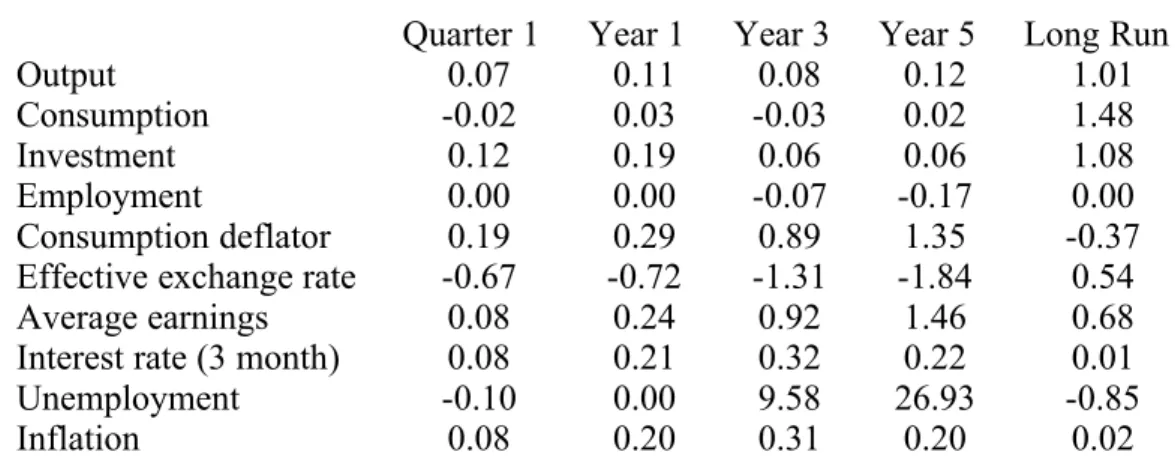
3.3 An increase in technical progress
Besides labour supply, the other main supply side shock which can be applied to the model is a change in technical progress. In the simulation reported in Table 3 the exogenous variable LETP (labour embodied technical progress) is raised by 1% throughout, implying a step increase in the level of the index of technical progress but no long run change in its growth rate.
The long run effects of this simulation should be very similar to the same increase in labour supply. However, there is a crucial difference in the short and
medium run effects which stem from COMPACT’s vintage production technology. As
technical improvements have to be embodied in new investment, this shock only influences the economy as new investment takes place. Since the maximum age of machines used in the simulation base is around 20 years, then it takes roughly this long before all machines benefit from the shift in technical progress.
Technical progress implies that less labour is required on new machines. This encourages investment, because new machines are now more efficient than the oldest machines being used. This in turn reduces marginal costs encouraging higher output and raising the price determined real wage (see Section 2.2 above). However, as new machines embodying the new technology come on stream, the average level of labour productivity rises (see Chart 3), which increases the real wage determined in the
labour market. In COMPACT the increase in the bargained real wage is greater than
that in the price determined real wage and so the NAIRU increases. The theoretical conditions under which an improvement in technical progress can raise the natural
effect has largely disappeared, and output completes its adjustment to a new level 1% above base.
{Chart 3 near here}
Another contrast between this simulation and the increase in labour supply concerns inflation in the short term. Whereas inflation falls when labour supply increases, because of the large rise in unemployment, in this simulation inflation increases slightly. This is in part because consumption anticipates future increases in output. This increase in inflation generates a rise in interest rates through the reaction function.
3.4 A temporary increase in world output
The simulation reported in Table 4 illustrates the response of COMPACT to a
temporary demand shock. World trade WTA and world output WINDP are both increased by 1% for 5 years. As this is a temporary shock, we keep nominal interest rates fixed. The increase in world output also raises world investment, which has important consequences for trade which we note below.
Chart 4a plots movements in non-oil exports and output. Although exports initially increase by 1%, there is a gradual decline over the next five years. This is in part due to an appreciation in the real exchange rate as UK prices rise, but also to a rise in the quality and variety of goods produced overseas as world investment increases. The increase in UK output is much less than 1%. In the first year the multiplier is about one, but towards the end of the five years it has declined to around one third. Initially import leakages combined with lower consumption are offset by higher investment and a stockbuilding accelerator, but these offsetting influences largely disappear after the first year.
{Chart 4a near here}
Chart 4b plots the path of consumption and inflation. Inflation initially jumps up, anticipating future levels of excess demand. It subsequently declines, as the future cumulated level of excess demand also falls. In the long run the price level comes close to returning to base, as the stock of nominal government debt (the model’s
nominal anchor in this simulation) is largely unchanged by this temporary shock. As a result, after two years inflation actually falls relative to base.
{Chart 4b near here}
As nominal interest rates are fixed, the pattern of consumption closely mirrors the behaviour of inflation. The steady decline in inflation over the first five years raises real interest rates, which through a Keynes-Ramsey type rule leads to higher growth in consumption. The initial jump in consumption is simply governed by the fact that discounted labour income is not greatly effected by this temporary shock.
4. Lessons and Future Developments
The motivation for building COMPACT came partly from a belief that a gap
had emerged between econometric macromodels and macroeconomic theory. For
example, when COMPACT was first built no other UK model included a consumption
function based on intertemporal optimisation. We believe that COMPACT has helped
to show not only that it is possible to construct an econometric model that is close to current theory, but also that the model can be used to inform the national policy
debate. Over the last four years COMPACT has been used not only to analyse the
effects of changes in UK monetary and fiscal policy (Church et al, 1997), but also to
examine the implications of changes in credit conditions (Darby et al, 1994), of
policies towards increasing investment (Driver and Wren-Lewis, 1995a), and exchange rate targeting (Driver and Wren-Lewis, 1995b, and Wren-Lewis, 1997).
The process of building and refining COMPACT also suggests some
observations which may have more general validity for model building. First, the construction of new models takes time, but it need not take that much time. The 18
months between start of work and completion for COMPACT, using a four person
team, may be a little misleading because it excludes some initial specification work, and most of the team had considerable experience in model building. On the other
hand the structure of COMPACT is fairly complex: not every macroeconometric model
needs to include a vintage production system, although we believe it is very important that at least some do given the additional layers of model properties and potential explanations of real world phenomena which can arise.
We found that the technique of theoretical deconstruction (see Wren-Lewis et
stressed above the use of this technique as a way of relating a model’s properties to simple theoretical paradigms, but it is also very useful as a development tool. Using this technique may occasionally reveal interesting macroeconomic insights, but in most cases it indicates problems with the model’s theoretical specification which need correcting.
Our current work on developing COMPACT involves a number of different
areas. One strand is investigating the consequences of imperfections in equity markets along lines suggested in a series of recent papers including Greenwald and Stiglitz, 1993. These authors argue that not only will bankruptcy risk be an important determinate of company sector decisions, but that at the general equilibrium level they could generate business cycles. Our initial line of attack will be to use data on bankruptcy rates as a proxy for perceived bankruptcy risk. Another area of work is attempting to identify asymmetries in price setting. Work on consumption is investigating potential effects from changes in the predictability of income. The model is also being extended to allow for endogenous growth effects. Finally a two-bloc version of the model is being constructed, where the calibrated second two-bloc will represent Europe. The two-bloc model can then be used to examine various issues related to UK entry into a European Monetary Union.
Table 1: Temporary Cut in Income Taxes
Quarter 1 Year 1 Year 3 Year 5 Long Run
Output 0.10 0.01 0.03 0.06 0.00
Consumption 0.12 0.12 0.13 0.20 0.00
Investment 0.19 0.17 0.02 0.02 0.00
Employment 0.01 0.02 0.03 0.02 0.00
Consumption deflator 0.03 0.07 0.20 0.15 0.01
Effective exchange rate -0.02 -0.02 -0.02 -0.02 -0.02
Average earnings 0.04 0.12 0.25 0.20 0.01
Interest rate (3 month) 0.00 0.00 0.00 0.00 0.00
Unemployment -0.46 -1.84 -5.18 -6.19 -0.09
Inflation 0.04 0.09 0.05 -0.07 0.00
Notes (i) Income tax rates reduced by 1 point for first five years of simulation. Fiscal feedback rule operates on income tax rates for remainder of simulation. Nominal interest rate fixed. (ii) All variables reported as % differences from base, except unemployment (000s difference from base) interest rates (% point difference from base), and inflation (% point difference from base).
Table 2: Permanent Increase in Population
Quarter 1 Year 1 Year 3 Year 5 Long Run
Output 0.28 0.46 0.63 0.78 1.00
Consumption 0.26 0.50 0.77 0.98 1.49
Investment 0.49 0.78 0.84 0.97 1.04
Employment 0.06 0.15 0.50 0.72 1.00
Consumption deflator 0.16 0.08 -0.50 -1.21 -0.26
Effective exchange rate -1.03 -0.99 -0.49 0.25 0.40
Average earnings -0.01 -0.09 -0.80 -1.56 -0.22
Interest rate (3 month) -0.06 -0.15 -0.36 -0.38 0.00
Unemployment 67.11 122.01 128.01 140.01 16.49
Inflation -0.06 -0.15 -0.34 -0.35 0.00
Notes (i) Population increased by 1% throughout simulation. Nominal interest rates endogenously determined by interest rate reaction function. (ii) For variable units see Table 1.
Table 3: Permanent Increase in Technical Progress
Quarter 1 Year 1 Year 3 Year 5 Long Run
Output 0.07 0.11 0.08 0.12 1.01
Consumption -0.02 0.03 -0.03 0.02 1.48
Investment 0.12 0.19 0.06 0.06 1.08
Employment 0.00 0.00 -0.07 -0.17 0.00
Consumption deflator 0.19 0.29 0.89 1.35 -0.37
Effective exchange rate -0.67 -0.72 -1.31 -1.84 0.54
Average earnings 0.08 0.24 0.92 1.46 0.68
Interest rate (3 month) 0.08 0.21 0.32 0.22 0.01
Unemployment -0.10 0.00 9.58 26.93 -0.85
Inflation 0.08 0.20 0.31 0.20 0.02
Notes (i) Labour embodied technical progress LETP increased by 1% throughout simulation. Nominal interest rates endogenously determined by interest rate reaction function. (ii) For variable units see Table 1.
Table 4: Temporary Increase in World Output
Quarter 1 Year 1 Year 3 Year 5 Long Run
Output 0.37 0.32 0.08 0.12 0.00
Consumption -0.05 -0.05 -0.08 0.04 0.00
Investment 0.67 0.54 -0.03 -0.01 0.00
Employment 0.03 0.05 0.08 0.03 0.00
Consumption deflator 0.05 0.14 0.26 -0.04 0.00
Effective exchange rate 0.00 0.00 0.00 0.00 0.00
Average earnings 0.12 0.28 0.35 0.00 0.00
Interest rate (3 month) 0.00 0.00 0.00 0.00 0.00
Unemployment -1.43 -5.53 -13.12 -13.33 0.16
Inflation 0.07 0.18 -0.01 -0.26 0.00
Notes (i) World trade and world output increased by 1% for 5 years. Nominal interest rates fixed. (ii) For variable units see Table 1.
References
Blanchard, O and S Fischer (1989) Lectures on Macroeconomics, MIT Press:
Cambridge, Massachusetts.
Carlin, W, A Glyn and J Van Reenan (1996) “Quantifying a Dangerous Obsession? Competitiveness and trade performance in an OECD panel of industries”, mimeo, University College, London.
Church, K, P Mitchell, P Smith and K Wallis (1993) “Comparative Properties of
Models of the UK Economy”, National Institute Economic Review No. 145 87-107.
Church, K, P Mitchell, P Smith and K Wallis (1995) “Comparative Properties of
Models of the UK Economy”, National Institute Economic Review No. 153 59-72.
Church, K, P Mitchell, J Sault and K Wallis (1997) “Comparative Properties of
Models of the UK Economy”, National Institute Economic Review No. 161 91-100.
COMPACT (1997) “COMPACT: a Quarterly Model of the UK Economy, version 3.0”,
mimeo, University of Exeter.
Darby, J, R Driver, J Ireland and S Wren-Lewis (1994) “Controlling Credit: The
Macroeconomic Consequences of Reversing Financial Liberalisation” New Economy,
Vol. 1 95-100.
Darby, J and J Ireland (1994) “Consumption, Forward Looking Behaviour and Financial Deregulation”, University of Strathclyde, ICMM Discussion Paper No.20 Darby, J, J Ireland and S Wren-Lewis (1995) “Interest Rates, Vintages and the Natural Rate”, ICMM Discussion Paper No.29
Darby, J, J Ireland and S Wren-Lewis (1997) “Technical Progress and the Natural Rate in a Vintage Model”, mimeo, University of Exeter.
Dornbusch, R (1976) “Expectations and Exchange Rate Dynamics”, Journal of
Political Economy Vol.84 1161-1176.
Driver, R and S Wren-Lewis (1995a) “The Investment Game”, New Economy, Vol. 2
104-109.
Driver, R and S Wren-Lewis (1995b) “Obstacles to EMU”, New Economy, Vol. 2
241-246.
Frenkel, J and A Razin (1992) Fiscal Policies and the World Economy, MIT Press:
Cambridge, Massachusetts.
Giovannini, A (1988) “The Real Exchange Rate, the Capital Stock, and Fiscal
Policy”, European Economic Review Vol.32 1747-67.
Greenwald B and J Stiglitz (1993) “Financial Market Imperfections and Business
Grossman, G and E Helpman (1991) Innovation and Growth in the Global Economy, MIT Press: Cambridge, Massachusetts.
Helliwell, J and C Higgins (1976) “Macroeconomic Adjustment Processes”,
European Economic Review, Vol.17 221-38.
Ireland, J and S Wren-Lewis (1992) “Buffer Stock Money and the Company Sector”,
Oxford Economic Papers Vol.44 209-231
Ireland, J and S Wren-Lewis (1994) “Inflation Dynamics in a New Keynesian Model”, University of Strathclyde, ICMM Discussion Paper No.24
Ireland, J and S Wren-Lewis (1998) “Exchange Rates, Nominal Inertia and Inflation”,
Scottish Journal of Political Economy, forthcoming.
Layard, R, S Nickell and R Jackman (1991) Unemployment: Macroeconomic
Performance and the Labour Market, Oxford University Press: Oxford
Leith, C and Wren-Lewis, S (1996) “Interest Rate feedback rules in an open economy with forward looking inflation” , University of Exeter Discussion Paper No.96/04 Leith, C, P Warren and S Wren-Lewis (1997) “Interest Rates and the Price Level”, University of Exeter Discussion Paper No.97/09
Leith, C and S Wren-Lewis (1997) “Optimal Disinflation in New Keynesian Models”, mimeo, University of Exeter
Moghadam, R and S Wren-Lewis (1994) “Are Wages Forward Looking?” , Oxford
Economic Papers Vol.46 403-424
Muellbauer, J and A Murphy (1991) “Measuring Financial Liberalisation and Modelling Mortgage Stocks and Equity Withdrawal”, mimeo, Nuffield College, Oxford.
Sargent, T and N Wallace (1975) “Rational Expectations, the Optimal Monetary
Instrument, and the Optimal Money Supply Rule”, Journal of Political Economy,
Vol. 83, 241-254.
Taylor, J (1993) Macroeconomic Policy in a World Economy, Norton: New York.
Turner, D. (1991) "The determinants of the NAIRU response in simulations of the Treasury model" , Oxford Bulletin of Economics and Statistics Vol.53 225-242 Wren-Lewis, S (1993A) “Macroeconomic Theory and UK Macromodels: Another Failed Partnership?”, University of Strathclyde, ICMM Discussion Paper No.9
Wren-Lewis, S (1993B) “What's so Bad about Borrowing?”, New Economy Vol.0
Wren-Lewis, S, J Darby, J Ireland and O Ricchi (1996) “The Macroeconomic Effects
of Fiscal Policy: Linking an econometric model with theory”, Economic Journal,
Vol.106 543-559
Wren-Lewis, S (1997) "The Choice of Exchange Rate Regime" , Economic Journal Vol.107 1157-1168
Appendix I: The Vintage Model15
COMPACT’s vintage production technology is vital in determining the model’s
medium run properties, including an important influence upon the NAIRU operating through the relationship between marginal and average productivity (see Section 2.2 above).
The vintage algorithm calculates the factor mix and productivity of each vintage of investment available to the firm. When the investment is undertaken, the factor mix is optimally chosen given an ex ante Cobb-Douglas production function and current and expected factor prices. As the factor mix is fixed ex post, expected discounted future labour costs XWC are important in this decision. Thus a future expected rise in wages will lead to a rise in XWC and so to a lower labour to capital
ratio in current investment. The temporary working variables vinyk and vinlk measure
the output to capital and labour to capital ratio on new machines. Labour embodied technical progress is assumed to grow at a constant rate.
The vintage algorithm calculates the maximum age of machine, MA, needed to produce a given level of output. It is assumed that given the dominant effect of embodied technical progress older machines are always less efficient, so all machines younger than the maximum age MA are used and none that are older. The algorithm also calculates the labour associated with each machine used, and the sum of these requirements is the labour requirement NSTAR. As existing labour can be used more intensively (e.g. overtime), and as there are convex adjustment costs in varying employment, actual employment N only adjusts gradually to NSTAR.
Next, the algorithm calculates the operating costs on the oldest used vintage. When smoothed with average costs to reflect firm heterogeneity this becomes a measure of marginal costs that determines the target level of prices PSTAR. As the price variable is a value added deflator, only labour costs are included in PSTAR.
Each period the firm is faced with the decision at the margin whether to produce output using the oldest machine, or instead invest in new machinery. Although new machines clearly have lower operating costs, their use involves bringing forward capital expenditure. The steady state level of the investment to output ratio (IYSTAR) involves two estimated terms in addition to a constant. The first compares the output to labour ratio on new and old machines. The second is the relative price of labour to capital. The dynamic investment equation assumes that there are quadratic costs in adjusting investment and in deviations from IYSTAR, so the investment to output ratio responds gradually to the discounted expected value of IYSTAR. Finally, the investment equation also includes a term in the current change in output i.e. an accelerator effect.
A permanent increase in real interest rates influences the long run investment to output ratio in two ways. Factor substitution implies a lower capital output ratio on new machines, thereby reducing the investment output ratio. In addition, higher interest rates will also reduce the optimum maximum age of machines used (see Darby et al, 1995), this has the effect of reducing the level of output associated with a constant level of investment and therefore raises the investment output ratio. The estimated parameter on relative prices in the IYSTAR equation captures both these effects, and its value is close to that implied by theory given the other parameters in the vintage model.
The equilibrium level of MA, and the ratio of marginal to average productivity, depend on the real cost of capital. Given the assumption of perfect capital mobility, this is mainly determined by the overseas real interest rate, but
15 The Borland Pascal subroutines which are used to solve the vintage model are available on the
because some capital goods are imported it is also a function of the real exchange rate. Through this route, changes in the real exchange rate can therefore influence the long run level of output via factor substitution, and also potentially via any induced changes in the equilibrium age structure of machinery.
Appendix II: The Model’s Equations16
This Appendix contains an alphabetical listing of COMPACT 3.0’s equations. A
complete listing of model variables and their mnemonics is provided in Appendix III. Where no estimation details are given, the equation was not estimated. This clearly applies to identities, but in addition a large number of minor model variables are simply assumed to grow in line with GDP or some other aggregate.
Most parameter values are ‘hard coded’ into the model, and can therefore not be changed without recompiling. An exception are the parameters shown as Par[x].
AFC Adjustment to factor cost, constant prices
Weights on main expenditure components, reflecting importance of indirect taxes in each.
AFC[t]=0.1690*CP[t]+0.0575*G[t]+0.0754*(I[t]+S[t]-S[t-1]) + 0.0363 *(XNO[t] +XO[t])
CA Current account Identity
CA[t]=(PXNO[t]*XNO[t]/100.0)-(PMNO[t]*MNO[t]/100.0)+(XO[t]-MO[t])*(PO[t]/ (EXDOL[t]*12.37588404)) + NPIO[t]
CDIV Dividends
Dividends are a function of post-tax profits (PROF), income taxes (TRINC) and the ratio of net assets (NFAC) to nominal income. There are a number of dummies reflecting changes in tax regime, dividend controls etc. A long-run coefficient of 1 is validly imposed on profits. The estimated equation below is overridden in two respects: the parameter on net assets is imposed and the estimated terms in the income tax rate are set to zero. The parameter on the term in the company sector net asset to GDP ratio is increased substantially from its estimated value to ensure that this ratio stabilises in simulations. It should be thought of as a proxy for similar terms in various company sector equations, along the lines of those estimated in Ireland and Wren-Lewis, 1992. The terms in the income tax rate lead to model instability in income tax simulations, and have therefore been set to zero pending re-estimation.
The dynamic structure was guided by a preference for smooth step responses and the avoidance of serial correlation.
Dln(DIV/PY)t= -0.94707 + 0.0099701 Q1 + 0.19331 Q2+0.013051 Q3
(0.18241) (0.0045501) (0.0046140) (0.0044914)
16 The data from the Office of National Statistics used in constructing and simulating COMPACT is
Crown copyright. It has been made available by the ONS through the ESRC Data Archive and has been used by permission. Neither the ONS nor the Data Archive bear any responsibility for the analysis or interpretation of the data reported here.
+ 0.20134 DD694 -0.33224 D7234 +0.38394 DUM79 -0.25365 D824
(0.043045) (0.044987) (0.45399) (0.062227)
- 0.13714D784 - 0.15459D752
(0.061763) (0.063298)
-0.32902Dln(DIV/PY)t-1 -0.18285Dln(DIV/PY)t-2 + 0.33520D[ln(DIV/PY)
(0.060304) (0.057901) (0.10810)
- ln(PROF)]t-2+ 0.82323 Dln(TRINC/100)t-1 -0.15184 D[DUMMY*
(0.32810) (0.056411)
-0.21302[ ln(DIV/PY)t-1- ln(PROF)t-1 ]-0.59056 ln(TRINC/100)t-1 +
(0.036849) (0.11506)
2000.0(NFAC/(PY*Y))t-1
Where:
PROFt = ln((GTPNO+GTPO)/PY) + ln(1-TRCORP)/100)
Q1, Q2 and Q3 are centred seasonal dummies.
DD694 = 1 in 1969:4 D7234 = 1 in 1972:3 and 1972:4
= -1 in 1970:1 = 0 Otherwise
= 0 Otherwise
DUM79 = 1 in 1979:4 DUMMY =1 before 1973:1
= -1 in 1980:2 = 0 Otherwise
= 0 Otherwise
D824 = 1 in 1982:4 D784 = 1 in 1978:4
= 0 Otherwise = 0 Otherwise
D752 = 1 in 1975:2
= 0 Otherwise
Estimation Period: 1969:1 - 1993:2 (98obs.)
Estimation Method: OLS
R2 0.79987
%SE 49.2566%
F(17,80) 18.8082[.000]
Diagnostic Tests:
Serial Correlation F(1,79) = 3.2445[0.075]
F(2,78)= 2.7205[0.072] F(3,77)= 1.8528[0.145] F(4,76)= 1.4573[0.224] F(8,72)= 0.95421[0.478]
Ramsey Reset F(1,102)= 0.04273[0.837]
Normality c2(2) = 183.239[0.000]
Heteroscedasticity F(1,105) = 0.30893[0.580]
ARCH F(1,79)= 0.27761[0.600]
CG Current grants
CG[t] = CG[t-1]*PC[t]/PC[t-1]
CHS Council house sales to persons
CHS[t] = PH[t]*CHS[t-1]/PH[t-1]
CMCHG Community Charge
CMCHG[t] = CMCHG[t-1]*W[t]*N[t]/(W[t-1]*N[t-1])
CP Consumers expenditure, constant prices
In an attempt to avoid heteroscedastic errors in the levels equation (the mean change and variance of consumption grow with the level of consumption) we scale both sides by lagged income in estimation. The instruments used were also scaled in a similar manner.
Generalised method of moments estimation is employed to account for the simultaneity between consumption and current income, the correlation between led consumption and contemporaneous variables with the error term and the MA(1) component of the error term induced by the quasi-differencing used to eliminate the term in unobservable human wealth. For more details see Darby and Ireland, 1994. A constant was allowed for in the determination of MRKUP, but its estimated value was negative and insignificant, and so it was set to zero.
Ct = d DVATX+ {Ct+1 - CGRt+1 - PROPt+1*(YECt+1 -
IPRt+1)}/{RRXt+MRKUPt} + [CGRt + PROPt(YECt -IPRt)]
+{ - [NWt + PROPt DBXMt]/[RRXt + MRKUPt]
+ [NWt-1 + PROPtDBXMt-1] + (1-PROPt)Yt}
Where:
Ct = CPt/POPt
DVATX = Dummy variable, = 0 except for
197204 = 1.0,197401 = 1.0,197403 = 0.5,197502 = -0.5 197901 = 1.0,197902 = -1.0,198001 = -0.75,198003 = -0.75 198704 = 1.0,199003 = 0.5,199101 = -0.5
CGRt = (CGt * 100/PCt)/POPt
PROPt = Exp(-a0 - a1*FLIBt)
YECt = {(WtNt13/1000 + TYPt[WtNt13/1000]/[WtNt13/1000 + NPIPt +
IPRt = (IPPt*100/PCt)/POPt
RRXt = Exp(0.25*Log(1+(RPOSTt - INFt)))
RPOSTt= RSHRt(1-TRINC/100)/100
INFt = (PCt+4 - PCt)/PCt
MRKUPt = K1*Exp(-a0-a1FLIBt)
DBXMt = [(GFAPt - NFAPt - MLPt)(100/PCt+1)]/POPt+1
NWt = [(NFAPt + HWPt)(100/PCt+1)}/POPt+1
Yt = {(WtNt13/1000 +ECt + TYPt[WtNt13/1000]/[WtNt13/1000 +
NPIPt + IPPt] - NICt - CMCHGt+}(100/PCt)/POPt
a0 a1 d K1
1.05006 3.44281 0.017891 -0.056434 0.154083
(0.264957) (0.786138) (0.00209911) (0.00416554) (0.034125)
E’HH’E = 0.101709
Estimation Period: 1969:1 - 1992:2
Estimation Method: GMM, MA(1)
Instruments used: 2nd, 3rd and 4th lags of consumption, current grants, net
wealth, debt, disposable income and FLIB. All instruments were appropriately lagged and scaled.
CTC Capital Transfers Companies
CTC[t] = (CTC[t-1]*PY[t]*Y[t])/(PY[t-1]*Y[t-1])
CTO Capital transfers overseas
CTO[t] = 0.0
CTP Capital transfers to personal sector
CTP[t] = (CTP[t-1]*PY[t]*Y[t])/(PY[t-1]*Y[t-1])
DNFAC Company sector NAFA
A quasi-identity: the budget constraint is not complete, and the missing elements account for the final term in nominal GDP.
DNFAC[t]=0.68943*GTPNO[t]+GTPO[t]-VIC[t]-CDIV[t]-TYC[t]+CTC[t]-
0.0*0.5*(NFAP[t]-NA[t]-NFAGM[t]+NFAP[t-1]-NA[t-1]-NFAGM[t-1])*(EXP(0.25*Ln(1.0+RS[t]/100.0))-1.0-Ln(PY[t]/PY[t-1])) +0.07*Y[t-1]*PY[t-1]/100
DNFAG Public sector NAFA
Identity apart from the residual error.
DNFAG[t] = - DNFAP[t] - DNFAC[t] + CA[t] - CTO[t]
DNFAP Personal sector NAFA Identity
DNFAP[t]=(W[t]*N[t]*13.0/1000.0)+EC[t]-TYP[t]-NIC[t]+0.23749*GTPNO[t] +NPIP[t]-(PC[t]*CP[t]/100.0)+CTP[t]-VIP[t] + CG[t] + NPREM[t]
EC Employers contributions
EC[t] = EC[t-1]*W[t]*N[t]/(W[t-1]*N[t-1])
EX Effective exchange rate
The imposed equation for EX embodies the uncovered interest parity condition with the possibility of a small term in the net overseas assets to GDP ratio reflecting a risk premium. This is currently set to zero.
The exchange rate equation can be viewed as an inverted demand function for net foreign assets. The coefficient on net assets therefore reflects the sensitivity of demand for net assets to the relative rate of return. As the parameter tends to zero, we approach perfect capital mobility. Attempts to estimate this parameter produce very poorly determined coefficients and so this parameter has been imposed at zero: however it can be altered to a small positive number without recompiling.
lnEXt = lnXEX1t + (RSQ - REUQ)t + 0.00(NA/(Y*PY))t
Where:
RSQ = -1 + Exp(0.25ln(1+RS/100))
REUQ = -1 + Exp(0.25ln(1+REU/100))
EXDOL US Dollar exchange rate
EXDOL[t] = EXDOL[t-1]*EX[t]/EX[t-1]
FLIB Financial liberalisation dummy
FLIB[t] = FLIB[t-1]
G[t] = G[t-1]*1.0038751
GA Gross overseas assets UK
In the short run GA changes with revaluations, but in the long run GA is a constant share of nominal GDP, allowing for an upward shift after the abolition of exchange controls.
GA[t]=GA[t-1]*(1.0-Ln(EX[t]/EX[t-1]))+(PY[t]*Y[t]/100.0)*( 0.54673 -0.21*EXDUM -0.051935*(GA[t-1]/(PY[t-1]*Y[t-1]/100.0)) )
Dummies: EXDUM =1 for 1973Q3 and earlier, 0 otherwise
GTPNO Gross trading profits, non-oil sector
GTPNO[t] = GTPNOS[t]*AYV
AYV=(PC[t]*CP[t]+PI[t]*I[t]+PYNO[t]*(G[t]+S[t]-S[t-1]-AFC[t])
+PXNO[t]*XNO[t]-PMNO[t]*MNO[t])/100 -GTPO[t]+(XO[t]-MO[t])*(PO[t]/ (EXDOL[t]*12.37588404))
GTPNOS Share of GTPNO in nominal non-oil income
A partial identity.
GTPNOS[t] = 1.0 - (W[t]*N[t]*13.0)/(BYV*1000) - EC[t]/BYV BYV=(PC[t]*CP[t]+PI[t]*I[t]+PYNO[t]*(G[t]+S[t]-S[t-1]-AFC[t])
+PXNO[t]*XNO[t]-PMNO[t]*MNO[t])/100 -GTPO[t]+(XO[t]-MO[t])*(PO[t]/ (EXDOL[t]*12.37588404))
GTPO Gross trading profits, oil sector
GTPO[t] = (PO[t]/(EXDOL[t]*12.37588404))*YO[t]*19.9125
HWP Housing wealth of persons
This is an imposed equation allowing for revaluations, depreciation, new investment and council house sales. (The coefficient on this last variable is greater than unity because CHS only covers England and Wales.)
(HWP/PH)t = 0.997509 (HWP/PH)t-1 + IHPt/100 + 1.138 (CHS/PH)t
I Investment, constant prices Identity
IHG Investment in public sector housing
IHG[t] = IHG[t-1]*0.9971474
IHP Housing investment persons
Estimated equation relating investment in housing to changes in the ratio of house prices to labour costs, and changes in the post tax real interest rate faced by house builders (RRSQ). Generalised Instrumental Variable Estimation (GIVE) was used since the inflation part of the real interest rate term was forward looking.
Dln(IHP)t = 0.96253 - 0.39193Dln(IHP)t-1 -0.48890Dln(IHP)t-2
-(0.62079) (0.12751) (0.11003)
0.23333Dln(IHP)t
(0.11070)
+ 0.74271 Dln(PH/(W+1000*EC/(13*N)))t-1 - 2.2553DRRSQt
(0.38507) (1.6843)
- 0.11425 ln(IHP)t-1 -0.91057 RRSQt-1 + 0.19616 D891
(0.076617) (0.50961) (0.084735)
Where:
RRSQ = Exp(0.25ln(1+(0.2+(1-TRCORP/100)*RS/100 - (PH(+4)-PH)/PH))))-1
D891 = 1 in 1989:1
= 0 Otherwise
Estimation Period: 1969:1 - 1992:2 (93obs.)
Estimation Method: GIVE
Instruments Used: RS, Inflation, TRCORP, Housing Starts, Orders for
New Housing.
R2 0.36546
%SE 79.6513%
F(8,85) 7.6954[.000]
Diagnostic Tests:
Serial Correlation c2(1) = 2.7244[0.099]
c2(2) = 5.0283[0.081]
c2(3) = 5.0636[0.167]
c2(4) = 5.4785[0.242]
c2(8) = 5.7967[0.670]
Ramsey Reset c2(1) = 0.0004[0.984]
Normality c2(2) = 2.7289[0.256]
INF Inflation (PYNO) Identity
inf[t] = 100*(pyno[t]/pyno[t-4]-1)
INO Non oil investment
The actual investment to output ratio is assumed to adjust slowly towards its desired value, IYSTAR, due to quadratic adjustment costs. (For an explanation of the dynamic form of this equation, see the equation for PYNO.) There is also a short-run accelerator effect allowed for in estimation. Estimation is by the generalised method of moments which is robust to MA(8) errors.
ln(INO/YNO)t = lln(INO/YNO)t-1 + ((1-l)2/(1-l9))*(ln(IYSTAR)t +
lln(IYSTAR)t+1 + l2ln(IYSTAR)t+2 + l3ln(IYSTAR)t+3+l4ln(IYSTAR)t+4
+ l5ln(IYSTAR)
t+5 + l6ln(IYSTAR)t+6 +l7ln(IYSTAR)t+7 + l8ln(IYSTAR)t+8 )
+ 0.771296Dln(YNO)t - 0.022690Dum
(0.679006) (0.013002) Where:
ln(IYSTAR)=-3.92317+0.539902ln[Vinyk*Weightedmc/(Vinlk*labc)] (1.54194) (0.845449)
+0.7ln[XWC/(PI*LETP)]
Dum = 1 between 1960:1 and 1983:3 l
= 0 Otherwise 0.935879
(0.069335)
Hansen’s Test of overidentifying restrictions: 1.53676[0.9088]
Estimation Period: 1977:1 - 1991:2
Instruments: Output, desired investment, investment output ratio, investment costs, wage costs, desired capital-output ratio, desired labour-capital ratio and wage costs relative to investment costs all lagged 9 periods.
INOC Cumulated INO
Proxy for variety and quality in trade volume equations. Uses a depreciation rate of 2% per quarter, as new product varieties can replace old varieties.
INOC[t] = INOC[t-1]*(1.0 - 0.02) + INO[t]
IO Investment in oil sector
IPP Interest payments on debt by persons
Personal debt multiplied by mortgage interest rates.
IPP[t]=(NMLP[t]+NMLP[t-1]+MLP[t]+MLP[t-1])*0.5* (EXP(0.25*Ln(1.0+RMORT[t]/100.0))-1.0)
IYSTAR Target INO/YNO ratio
IYSTAR[t]=exp(3.92317+
0.539902*ln(vinyk[t]*weightedmc(t)/(vinlk[t]*labc[t]))+ 0.7*ln(XWC[t]/(PI[t]*LETP[t])) )
LETP Labour Embodied Technical Progress
LETP[t] := exp(ln(LETP[t-1]) + ln(1.0+LETPR)) LETPR := exp(0.25*ln(1.+1.0/100.0)) - 1 to 1989Q4 LETPR := exp(0.25*ln(1.+2.0/100.0)) - 1 from 1990Q1 Starting value of series is 1 in 1902Q1
MA Maximum age of vintage in use
calculatema is a subroutine/procedure in the vintage model. ma[t] = calculatema(t)
MAVPNY Marginal to average N/Y
A constructed, post recursive variable, measuring the ratio of marginal and average costs. This is important in determining the NAIRU.
mavpny[t] = pstar[t]*yno[t]/(w[t]*n[t] +1000*ec[t]/13.0)
MLP Mortgage liabilities persons
MLP grows with housing wealth, with an additional influence from financial liberalisation.
The dynamics in this equation (D4 and D2) reflect the nature of the two explanatory
variables: HWP and FLIB are both interpolated from annual data series. Four-period differencing avoids the introduction of spurious quarter on quarter dynamics which would otherwise induce serial correlation.
D4ln(MLP/HWP)t = - 0.066052+ 1.17581D4ln(MLP/HWP)t-1 +
(0.023423) (0.114378)
(0.1059016) (0.0749852)
- 0.040285 ln(MLP/HWP)t-1 + 0.049127 FLIBt-1
(0.0143363) (0.019495) - 0.60759 DUM72+ 0.035743 DD744- 0.045752 DD884
(0.090281) (0.0077199) (0.0076126)
Where:
DUM72 = 0.5 in 1972:1 DD744 = 1 in 1974:4
= -0.5 in 1972:4 = -1 in 1975:1
= -1 in 1973:1 = 0 Otherwise
= 0 Otherwise
DD884 = 1 in 1988:4
= -1 in 1989:1 = 0 Otherwise
Estimation Period 1969:3 1990:4 (86 Obs)
Estimation Method: OLS
R2 0.97997
%SE 14.15%
F(8,77) 520.9467[.000]
Diagnostic Tests:
Serial Correlation F(1,76) = 0.1276E-3[0.991
F(4,73) = 0.15688[0.959] F(8,69) = 1.7468[0.103]
Ramsey Reset F(1,76) = 0.4.1354[0.045]
Normality c2(2) = 0.36692[0.832]
Heteroscedasticity F(1,105)= 0.60169[0.440]
ARCH F(1,76) = 0.24860[0.620]
F(4,73) = 0.98508[0.421]
MNO Non oil imports
The MNO equation models the share of imports in demand as a function of competitiveness, the ratio of domestic cumulated investment to world cumulated investment and a variable reflecting the general growth in world trade relative to world income.
DMDNOt = -0.032202- 0.22913 MDNOt-1 + 0.024663 ln(PYNO/PMNO)t-1
(0.015378) (0.049508) (0.0075719)
+ 0.0063275(WTA/WINDP)t - 0.031909 ln(INOC/WIMC)t