1081.pdf

ABSTRACT

A three-dimensional model for the simulation of transient groundwater flow is devel¬ oped. The model is called REGFED for REGional flow using Finite Elements and Dif¬ ference methods. A review of groundwater flow and contaminant transport concepts and theory reveals that three-dimensional representation of groundwater systems is essential for realistic simulation of flow and transport. From an analysis of currently available

ground-water flow models and algorithms, it is apparent that a mixed numerical method consisting

of finite-elements and finite diff"erences is a suitable method for solving the groundwater

flow equation in three dimensions. An algorithm known as ALALS (Alternate sublayer

And Line Sweep) is selected for the basic model algorithm.

Finite elements are applied to areal components, and flnite differences are applied to vertical components of flow. The model accomodates both conflned and unconfined groundwater flow problems and is also capable of handling the draining and refilling of individual elements or entire layers. Because of the model's efficient algorithm, it can accomodate thousands of nodal unknowns with minimal computer storage and CPU time. Quasilinear unconfined groundwater flow problems are solved using a Picard iteration scheme. Entire confined layers are skipped in the iteration scheme in order to decrease the CPU time required to solve the problem. The model is validated under a wide assortment of conditions including confined flow, confined flow with partially screened wells, unconfined

flow, combined confined/unconfined flow, and flow with drained and refilled layers. A

heuristic error analysis shows that model results compare well with validation results. Mass-balance errors for various groundwater flow problems are minimal for most cases.

The convergence speed and stability of the iteration scheme is evaluated for solu¬ tion of unconfined groundwater flow problems. A benchmark comparison using sample groundwater flow problems was performed with the REGFED model and with the USGS McDonald-Harbaugh model. Example applications further demonstrate the flexibility of the model.

TABLE OF CONTENTS

Table of Contents ... ii

List of Figures... iv

List of Tables... vi

Acknowledgements... vii

1. Introduction ... 1-1

1.1 Background and Motivation ... 1-1

1.1.1 Relationship between Groundwater Flow and Contaminant Transport 1-1 1.1.2 Importance of Modeling Flow in Three Dimensions ... 1-5

1.1.3 Importance of Modeling Unconfined Flow... 1-9

1.2 Research Goal and Objectives ... 1-13 1.3 Methodology... 1-15 2. Theoretical Background and Literature Review... . Z'i 2.1 Governing Equations for Groundwater Flow ... 2-1 2.1.1 Theory: Darcy's Law... . 2-1 2.1.2 Theory: Groundwater Flow Equation ... 2-2 2.1.3 Theory: Unconfined Groundwater Flow ... 2-4 2.2 Solutions of Groundwater Flow Equations... 2-5 2.2.1 Analytical Flow Models ... 2-5

2.2.2 Numerical Flow Models ... 2-6

2.2.3 Indirect Velocity Estimation ... 2-12 2.2.4 Direct Velocity Estimation... 2-14 3. Development of Confined Flow Model ... 3-1 3.1 Overview of Model Algorithm ... 3-1 3.2 Derivation of Algorithm... 3-2 3.3 Application of Boundary Conditions and Source and Sink Terms .... 3-13

3.4 Matrix Solution Methods ... 3-16 3.5 Other Model Features... 3-18

3.5.1 Steady-State Case...,... 3-18

3.5.2 Mass Balance Computation... 3-19 4. Development of Unconfined Flow Model ... 4-1 4.1 Overview of Model Algorithm ... 4-1

4.2 Picard Iteration... 4-3

4.3 Skipping Confined Layers ... 4-6 4.4 Draining, Refilling Selected Nodes... 4-8

4.5 Storage Estimation... 4-12

5. Testing of Model Accuracy and Sensitivity ... 5-1

5.1 Confined Flow... 5-2

6. Model Applications ... 6-1

6.1 Two-Well Tracer Test... 6-1

6.2 Flow within a Multi-Level Monitoring Well... 6-4 6.3 Flow in an Aquifer/Aquitard Groundwater System ... 6-7 6.4 Comparison with McDonald-Harbaugh Model ... 6-10

7. Conclusions and Recommendations... 7-1 7.1 Conclusions... 7-1 7.2 Recommendations... 7-1 8. Notation... 8-1 9. References ... 9-1

LIST OF FIGURES

1.1 Heterogeneities Influencing Dispersion... 1-6

1.2 Typical Three-Dimensional Groundwater Flow and Transport Problem . . 1-8

1.3 Vertical Variations in Hydraulic Conductivity... 1-10

1.4 Hypothetical Layered Aquifer... 1-11

1.5 Comparision of Vertically Averaged and Layered Contaminant Transport

Simulations... 1-12

1.6 Confined and Unconfined Aquifers ... 1-14

2.1 Effect of Semi-Confining Layer on Groundwater Flow... 2-10

3.1 Three-Dimensional Discretization of Aquifer Domain ... 3-4

3.2 Block-Centered Approach ... 3-7

3.3 Linear Triangular Finite Element... 3-11

3.4 Flow Diagram for ALALS Algorithm ... 3-14

3.5 Typical Boundary Conditions for Groundwater Flow ... 3-15

3.6 Flow Diagram for Steady State Case... 3-20

4.1 Schematic Represntation of Saturated Thickness ... 4-4

4.2 Flow Diagram for Picard Iteration ... 4-7

4.3 Illustration of Layer-Skipping... 4-9

4.4 Flow Diagram for Layer-Skipping... 4-10

4.5 Draining and Refilling of Nodes... 4-11

4.6 Flow Diagram Draining/Refilling Nodes... 4-13

4.7 Unconfined/Confined Nodes ... 4-15

5.1 Single Pumped Well, Radially-Symmetric, Homogeneous Aquifer . . . 5-3

5.2 Comparison of Analytical and Numerical Solutions: Confined Flow .... 5-5

5.3 Partially Penetrating Well... 5-7

5.4 Comparison of Analytical and Numerical Solutions: Partially Penetrating Well 5-8

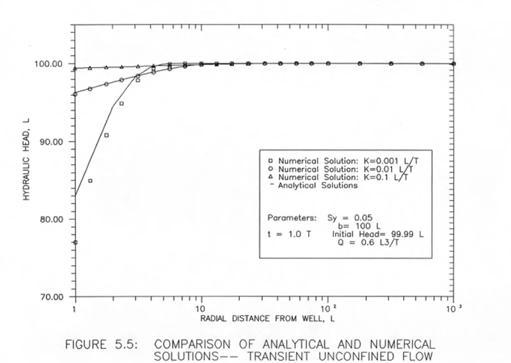
5.5 Comparison of Analytical and Numerical Solutions: Unconfined Flow . . . 5-11

5.6 Illustration of Steady State, One-Dimensional Unconfined Flow... 5-12

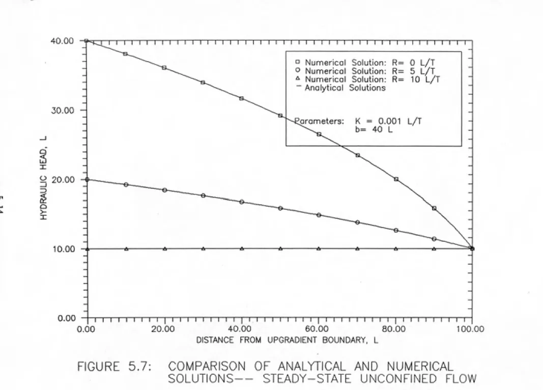
5.7 Comparison of Analytical and Numerical Solutions: Steady State Unconfined Fldavl4

5.8 Comparison of Analytical and Numerical Solutions: Steady State Unconfined Flow

with Recharge... 5-15

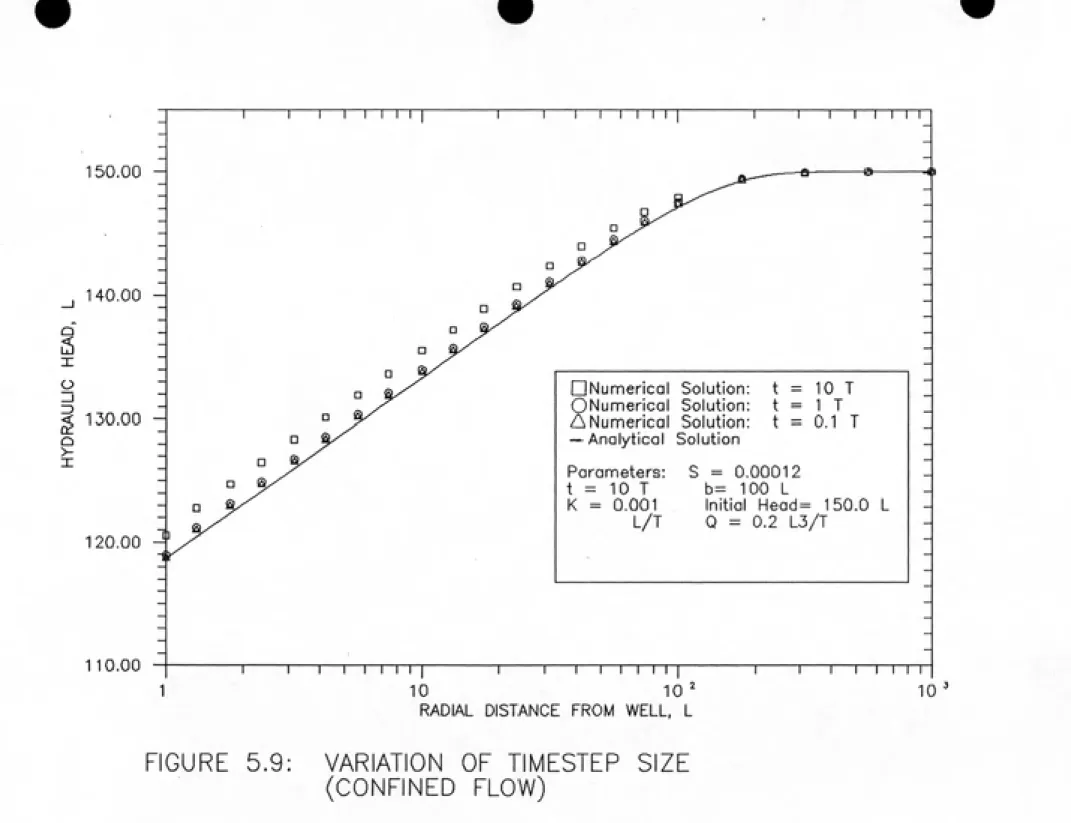
5.9 Variation of Model Parameters: Timestep Size (Confined Flow)... 5-18

5.10 Variation of Model Parameters: Horizontal Discretization (Confined Flow) 5-19

5.11 Variation of Model Parameters: Vertical Discretization (Confined Flow) . . 5-21

5.12 Variation of Model Parameters: Maximum Allowable Error (Unconfined Flow) 5-22

5.13 Variation of Model Parameters: Maximum Allowable Iterations (Unconfined

LIST OF TABLES

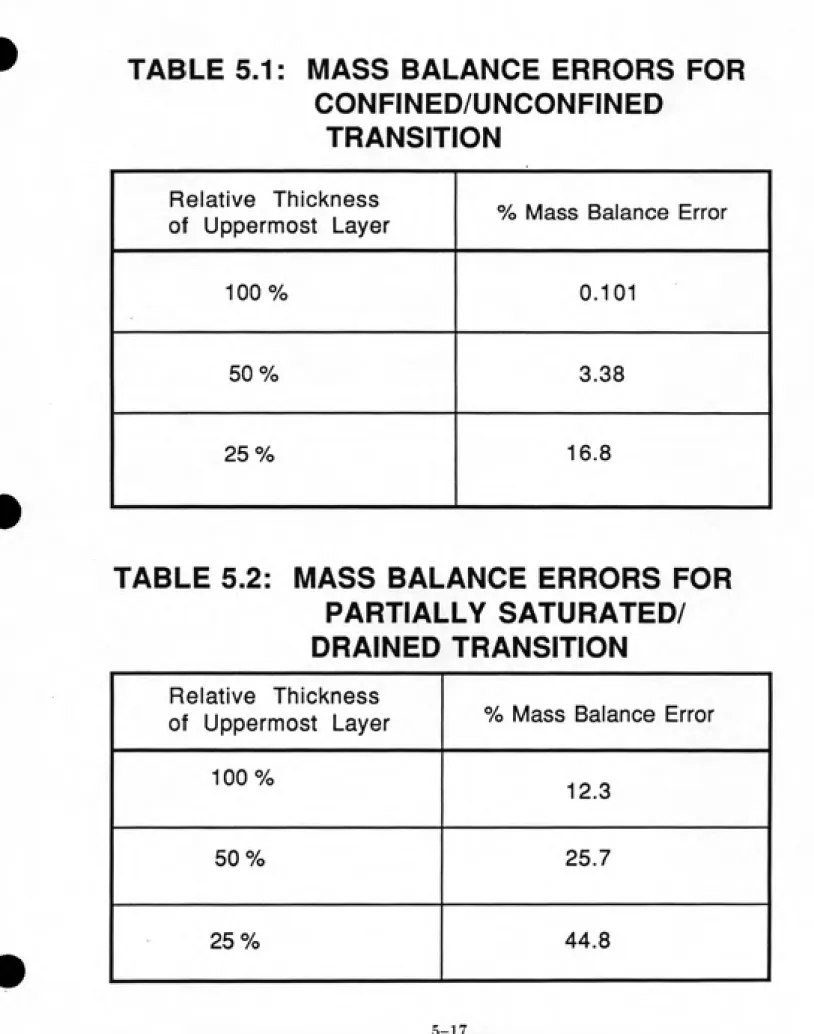
5.1 Mass Balance Errors for Confined/Unconfined Transition... 5-17

5.2 Mass Balance Errors for Partially Saturated/Drained Transition ... 5-17

5.3 Parameters Used in Test Cases... 5-28

ACKNOWLEDGEMENTS

Thanks first to my intrepid advisor. Dr. Cass T. Miller. Without his encouragement

and guidance, this research never would have gotten off the ground. He has helped reveal to me the many fascinating facets of the groundwater field.

To my office-mates, thank you for bearing with me. Thanks especially to Joe Pedit for his valuable insight and reminders that this isn't the most important thing in the world.

But most of all, thank you Harriet for your love and support. I couldn't have done it

1 INTRODUCTION

1.1 Background and Motivation

Approximately half the population of the U.S. depends on groundwater for its drink¬

ing water supplies. There is growing evidence that this resource, once thought to be

contaminant-free, is being contaminated by municipal, industrial, and agricultural wastes.

Researchers are thus focusing upon studying the mechanisms responsible for contaminant

transport in groundwater systems. To prevent the further deterioration of groundwater

quality, researchers are developing methodologies for monitoring, analyzing, and predict¬

ing the movement of contaminants in the subsurface. Predictive models of groundwater

contaminant transport can provide the information needed for the accurate assessment of

health risks resulting from contamination of drinking water supplies, or for the design and

evaluation of measures for renovating contaminated groundwater aquifers.

1.1.1 Relationship between Groundwater Flow and Contaminant Transport

One of the most important factors in predicting the movement of contaminants in

models can be developed in the context of groundwater contamination problems.

In order to understand the relationship between groundwater flow and contaminant

transport, one must examine the equations that govern the hydrodynamics of contam¬

inant transport. Determinstic and stochastic approaches for mathematically describing

contaminant transport are possible. This report focuses upon deterministic apporaches

for transport and flow, due to the relative difficulty of applying the stochastic approach to

practical contaminant transport problems.

The advective-dispersive equation is generally considered to be the equation that

governs contaminant transport (Anderson, 1979), although other researchers have proposed

different approaches (Gillham et al., 1982; Tompson, 1986). The advective-dispersive

equation considers solute flux to be the result of the average bulk movement of the fluid in

the direction of groundwater flow (advection) and a Fickian-type mixing in the displacing

fluid (dispersion) (Gillham et al., 1984). For saturated flow in heterogeneous porous media,

the general form of the advective-dispersive equation is written as

^ = V . (D . VC) - V. VC + (^) + T{C) (1.1)

where

C — solute phase concentration [MjL^)

t = time (T)

V — vector of average groundwater pore velocity {L/T)

D = hydrodynamic dispersion tensor {L'^/T)

V- = divergence operator

V = gradient operator

(W)rin = reactive term (M/L^/T)

Reactive processes such as sorption, chemical reactions, and biological degradation can

play important roles in the fate of contaminants and should also be accounted for in any

model of non-conservative groundwater contaminant transport. The focus of this report is

not on the reactive portion of Equation 1.1, but concentrates on the the hydrodynamics.

The conservative form of Equation 1.1 implies that

(

which reduces Equation 1.1 to

^ = v-(D •vc)-tr-vc + r(c) (1.3)

Bear (1972) describes the hydrodynamic dispersion tensor as the sum of two compo¬

Dij = arvSij + {ai - aT)viVj/v + D* (1,4)

where

Dij = i,j term of dispersion tensor [L^ /T)

i,j = components of Cartesian coordinate system ar — transverse dispersivity (L)

ai = longitudinal dispersivity (L)

V = average groundwater pore velocity {L/T)

D*

ͣ

= effective molecular diffusion coefficient [L^ /T)

Sij = Kronecker delta function [dimensionless]

= 0 for i 7^ j

The product of dispersivity and flow velocity is known as the mechanical disper¬ sion component. The mechanical mixing is a process introduced by averaging irregular

advective displacements taking place within the porous groundwater matrix (Fried and

Cornabous, 1971). In active groundwater flow through a granular medium, mechanical

dispersion is usually dominant over diff'usion, and so the D* term is often a relatively

small component.

By examining Equation 1.2, one can see that groundwater velocity, through the advec¬ tive term, is a crucial part of the advective- dispersive approach to modeling contaminant transport, for a typical groundwater aquifer. In addition, Equation 1.4, which describes the dispersion tensor, includes velocity-dependent terms.

Various mathematical solutions to the advective-dispersive equation have been pro¬ posed. These solutions have been compared to experimental results from laboratory-scale soil columns. The solutions have been shown to provide accurate representations of conser¬

vative solute transport, under laboratory conditions (Gillham et al., 1984). Longitudinal

dispersivities have been found that range within a couple of orders of magnitudes of each

other ( 10""* to 10""^ meters). However, when the solutions of the advective-dispersive

equation are applied to fleld-scale tracer tests, longitudinal dispersivities in the range of

1 to 100 meters have been commonly reported (Gelhar et al., 1985). This variation in

the advective-dispersive equation.

The discrepancies between longitudinal dispersivities obtained from laboratory- and field-scale experiments have led some researchers to conclude that dispersivity is a pa¬

rameter which is scale-dependent (Fried, 1975; Feaudecerf and Sauty, 1978; Sudicky and

Cherry, 1979; Pickens and Grisak, 1981). The scale dependency is generally attributed

^

Heterogeneities can be found in a range of scales in the geological media. Figure 1.1

illustrates various types of heterogeneities that occur and the subsequent effect on velocity

distributions. These heterogeneities affect the velocity field, and therefore groundwater

flow, at all scales. Figure 1.1 illustrates that heterogeneities can occur from the grain-size

scale to the geologic- layering scale. The layering scale could, if necessary, be identified

and mapped by careful drilling, sampling or geophysical logging. If the smallest scale of

heterogeneities in a deterministic-type media could be identified and accounted for, then

the differences in advection or groundwater flow could be accurately simulated. However,

these heterogeneities cannot be identified by conventional methods of field testing (Freeze

and Cherry, 1979). As long as the smallest heterogeneities cannot be identified, it is

important that models of groundwater flow provide accurate simulations, using the best

available information from the scales that can be identified.

The dispersivity parameter is a result of averaging over scales larger than the smallest

scales. The average linear groundwater velocity that is used as input to the

advective-dispersive equation reduces the individual velocities in the interstitial flow paths to a

single value (Freeze and Cherry, 1979). Averaging of velocities often goes one step further

where individual velocities within layers of different hydraulic conductivities are averaged

to a single value. The result of this averaging is that the observed dispersity parameters

contain the deviations in velocities at the scale over which the flow has been averaged

(Anderson, 1984). Deterministic models of the advective-dispersive equation cissume that

hydrodynamic process occur over measurable scales. If the models included the smallest

heterogeneities, theoretically there would be no deviations in velocities over a small scale,

and therefore the dependence of prediciting hydrodynamics on dispersivities would be

reduced.

ass^-#

FIGURE 1.1

DISPERSION PHENOMENA

Mixing in individual pores

••SSi-v.-^^v::

Mixing by molecular

diffusion

Mixing of pore channels

Higher

avers

Macrodispersive Spreading ^ Iimiobile Fluid

The majority of contaminant transport models have been developed over two dimen¬

sions (Burnett and Frind, 1987). In these cases, important aquifer properties such as

velocity magnitudes and directions are spatially averaged over the relevant dimensions

(usually the vertical dimension). This approach dooms the prediction of contaminant

transport to failure, in all but the simplest of groundwater systems. Figure 1.2 provides

a schematic illustration of a typical three-dimensional groundwater flow and contaminant

Various researchers have reported that three-dimensional modeling of flow and con¬

taminant transport improves the accuracy of such simulations relative to two- or

three-dimensional simulations. Stochastic analyses performed by Freeze (1975) and Gelhar

(1976) show that there is considerably less variation about a mean hydraulic head value

for three-dimensional flow models than for two- and one-dimensional models. Increases in

these variations tend to inflate the value of dispersion and produce poor predictive ability

The scale eff"ects on dispersion that were discussed previously may be an artifact of

the dimensionality of the models employed to predict dispersion (Domenico and Robbins,

1984). Results of Domenico and Robbins (1984) indicate that a "scaling-up" of dispersivity

will occur when the dimensionality of a model fails to match that of a natural system.

Molz et al. (1983) conclude that the vertical distribution of hydraulic conductivity (and

the subsequent effect on mixing) is a key parameter that aff"ects overall dispersivity.

Burnett and Frind (1987) describe variations in hydrodynamic parameters in three

dimensions that influence the shape of a contaminant plume. Arnett et al. (1977) report

that three-dimensional models of contaminant movement compare better with observed

contaminant movement at the Hanford, Washington site, than for two-dimensional models.

Vertically-layered groundwater systems are often found in the field (Huyakorn et al.,

FIGURE 1.2

TYPICAL 3-D GROUNDWATER FLOW AND TRANSPORT PROBLEM

INFILTRATION

AQUIFER 1

lAQUITARD 1

LANDFILL

AQUIFER 2

^____________

^^^^^^2^^^

^^^^^^^^Ml

AQUIFER 3

W^^s^^^^^^^^^^^^^

^i^^:^;^^^^^^^^;^:^^^^^J

CROSS-SECTIONftL

VIEW

\

INFLOW

LANDFILL

orders of magnitude (Sudicky, 1986). If the variations in flow caused by the differences are

not taken into account, at best only averaged contaminant concentrations can be predicted

rather than in the individual layers. The presence of a high conductivity layer may direct

the contaminants toward this layer, the effects of which may be ignored in a one- or

two-dimensional analysis. Results from Sudicky (1986) and Molz (1986) showing the vertical

distribution of hydraulic conductivities are shown in Figure 1.3. These results show that

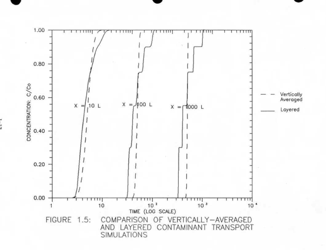
hydraulic conductivity, and thus velocities, can vary more than an order of magnitude in

The effects of the vertical averaging of groundwater velocity distributions can be

shown through some hypothetical simulations. An analytical model of the one dimensional,

conservative form of the advective-dispersive equation (Bear, 1979) was applied to two

cases: 1) a five-layer aquifer, with each layer having a different groundwater velocity, and

a line source of contaminant, as shown in Figure 1.4; and 2) the same aquifer, but with

the velocities of the five layers averaged into a single value of velocity. The simulations

were performed at three different positions down-gradient from the contaminant source.

The value of longitudinal dispersivity for the second case was fitted to the results from the

first case at the first down-gradient position. All other parameter values were the same for

each case.

The results are shown in Figure 1.5 (note that the time axis has a log scale). These

results show that, at the first position (where the dispersivity was fitted), the vertically

averaged results resemble the non-vertically averaged resits. However, cis the simulations

move farther from the contaminant source, the vertically averaged results no longer resem¬

ble the non-vertically averaged results. Thus, the vertical variations cannot be averaged

while expecting the simulations to provide accurate results.

1.1.3 Importance of Modeling Unconfined Flow

FIGURE 1.3

VERTICAL VARIATIONS IN HYDRAULIC CONDUCTIVITY

After Sudicky (1986) and Molz (1986)

219.231 M.om 211.138 - 2tl.5«

n

" 2H.238

c

g 2lt.0«

> 217.738

r Core 15

«j

HIT _T1IIIIJ

I ͣ ...1 ,...'"I ..."^

21S.3* 213.095 218.M5

r Core 16

— 2t8.S9B

" 2H.J6

e

g 211.095

> 2l7.i«

-U 10 10 10 Hydraulic Conductivity (ca/s)

I I Miim—I I "I iimi ' ' ' "'1'

217.595 217.3«

-10 ͣ 10

Hydrau1i c Conduct i v i ty

10

(ca/s)

• MO.7)

• M 3 8) ..I'i 6.6)

• (ͣ; 9 91 .115 2.9)

.IS6,0 159.0)

FIGURE 1.4

HYPOTHETICAL LAYERED AQUIFER

CONTAMINANT SOURCE

V= 3.0

V = 2.0 L/T

§

V = 1.0 L/T

PARAMETERS

Retardation =1.0

Longitudinal Dispersion = 1.0

LT

5 Layers

Layer Thicl<ness

= 0.2 L

^

x = 10 L X = 100 L X = 1000L

Is5

O

o o

<

o O

o

1 .uu —

...r r r ii iii| /' \r\

1 1 mT| -.I' in 1 mil 1 1 II 1 mf...1 1 1 1 1 III

/

_/

1 /

1

1

h(

1 .—ͣ' ₁

-ll \ \ 1

-0.80 - 1

\

J (

:

i

0.60

-\

_J

-X =/ 10

X =JfOO L

1000 L

-i

1

-0.40 - M 1

;

\\

[-1 1

1

—

0.20 - /

/

1

-/

1'

:

n r\r\

1 y

U.UU _{1 lllll}

I'i 1 1 _{1 1 1111 (} 1 1 1 1 1 _{II i| 1} 1 1 1 1 1II

— Vertically Averaged __ Layered

1 10 10' 10^ 10*

FIGURE 1.5: COMPARISON OF VERTICALLY-AVERAGED

table). Flow in confined aquifers is bounded above and below by impervious layers.

Un-confined aquifers are bound below by an impervious layer, but are bound above by the

top of the water table. Figure 1.6 shows a schematic representation of the two types of

aquifers. Most contamination cases can be found in unconfined aquifers, due to the lack

of a protective confining layer and thus an increased vulnerability over confined aquifers.

Shallow unconfined aquifers are particularly susceptible to pollution from contaminants

when little or no treatment is afforded by the overlying strata (Guvanasen and Volker,

1981).

However, most of the available flow models either do not accomodate unconfined flow

at all or do so unreliably. Modeling an unconfined groundwater system as a confined

system usually is inaccurate because the flow regimes may differ greatly between the two

types of systems. The presence of a free upper boundary in an unconfined aquifer can

significantly affect groundwater velocities, especially in shallower aquifers. These differ¬

ences can translate to poor estimates for the movement of groundwater contaminants, if

the wrong system is modeled.

1.3 Research Goals and Objectives

Thus, the goal of this research is to develop a versatile model that accurately and

efficiently simulates confined and unconfined groundwater flow in three dimensions.

The objectives to be met with this research are:

1) To develop a three-dimensional numerical model for simulating confined

ground-water flow.

2) To develop a three-dimensional numerical model for simulating unconfined

ground-water flow, using the confined flow model for the basic structure so that a combination

of confined and unconfined flow can be accomodated in the final model.

3) To test the accuracy of both the confined and unconfined flow portions of the final

FIGURE 1.6

CONFINED AND UNCONFINED AQUIFERS

sz

WATER TABLE

d

UNCONFINED AQUIFER

ilENTIOMETRIC

SURFACE

4) To apply the model to some hypothetical groundwater flow situations.

1.3 Methodology

To meet the first objective, an algorithm consisting of a numerical solution of the

groundwater flow equation is selected. This algorithm, called the ALALS algorithm (for

ALternate sublayer And Line Sweep procedure) has been described in the literature. The

complete derivation of this algorithm is performed. Next, a structured and commented

computer code that incorporates the ALALS algorithm is developed. Various modifications

of the algorithm are also included in the code, such as the ability to simulte steady-state

as well as transient problems, and a provision for calculating mass balance errors. The

result is a model for simulating confined flow.

The model developed under the first objective is then modified to include unconfined

flow. The equation describing unconfined flow is not linear, as it was the confined case.

An iterative algorithm (Picard iteration) is utilized to solve the unconfined flow equation.

Application of the iterative algorithm results in a significant increase in computaional

effort over the confined model. The computational eff^ort is reduced by modifying the

iterative algorithm to include unconfined aquifer layers only. Other problems resulting

from modeling unconfined flow, such as the draining and reflUing of aquifer layers, are

incorporated into the model. The resulting model can simulate confined and unconfined

flow separately or at the same time. The model is named REGFED for REGional flow

using Finite Element and Differences methods.

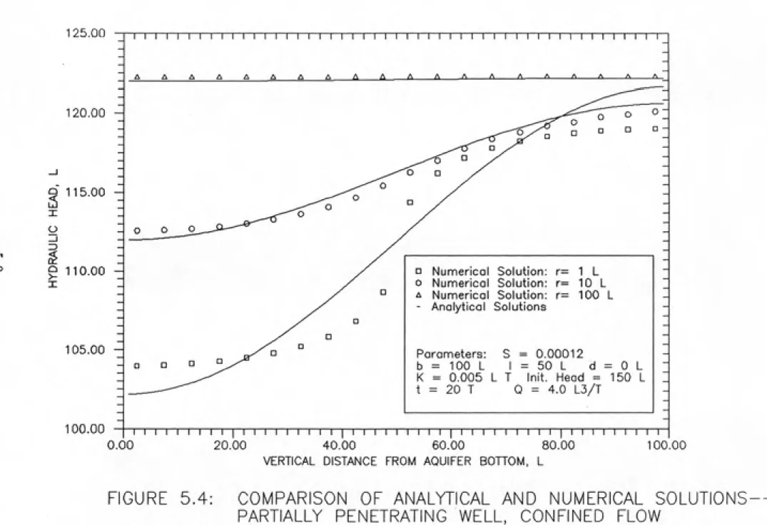
The third objective involves testing the accuracy of the unconfined and confined por¬

tions of the model. In this research, accuracy is evaluated by graphical comparisons of

model results with results from analytical solutions. In a few cases where analytical mod¬

analyzed by graphical comparisons of model results with analytical solution results.

Hypothetical applications are simulated with the model. The example applications

include flow within a monitoring well, flow in an aquifer-confining layer system, and flow

resulting from a two-well tracer test. In addition, the performance of the model is com¬

pared to the most popular three-dimensional public domain groundwater flow model, the

McDonald-Harbaugh model. This comparison provides a way to gauge the relative effi¬

ciency of the WELFED model. The total computational time required for each model to

2 THEORETICAL BACKGROUND AND LITERATURE RE¬

VIEW

The determination of groundwater flow requires the evaluation of either or both of

the hydraulic head variable or the velocity variable. Hydraulic head is a measure of fluid

potential; it consists of the sum of a pressure head and an elevation head. Most groundater

flow models simulate distributions of hydraulic heads. Groundwater velocity is the velocity

variable found in the advective-dispersive equation. Velocity is proportional to the negative

of the groundwater gradient (Darcy's Law).

Generally, there are two approaches towards simulating groundwater flow velocities:

the indirect and direct method. The indirect method- the most popular- consists of sim¬

ulating hydraulic head distributions and then using Darcy's Law to approximate

ground-water velocities. The direct method uses Darcy's Law directly to simulate groundground-water

velocities. This report focuses on simulating distributions of hydraulic heads.

Before discussing the approaches toward obtaining hydraulic head and velocity, the

classical theories of groundwater flow should be reviewed. By examining the theory first,

one can understand the necessary steps in each approach.

2.1 Governing Equations for Groundwater Flow

2.1.1 Theory: Darcy's Law

, = -k|^ m

where

q = specific discharge (L/T)

K = hydraulic conductivity [L/T)

h — hydraulic head (L)

1^ = groundwater gradient [dimensionless]

Darcy's law is valid for groundwater flow in any direction in space. However, it should

be understood that the specific discharge calculated from Darcy's Law is a macroscopic

concept, which is averaged over a portion of the porous medium. The specific discharge is

clearly diff"erentiated from the velocities encountered in the actual path of the fluid particle

through a porous medium (Bear, 1979).

The average velocity, v, represents the flow that passes through only the portion of

the porous medium occupied by voids in the porous matrix. The average velocity is found

in the advective and dispersive terms of the advective-dispersive equation. It is obtained

by

tJ = - (2.2)

where

V — average groundwater pore velocity [LfT]

n — porosity [dimtnsionltss)

The continuity equation for groundwater flow is a partial differential equation that

describes the conservation of fluid mass during flow through a porous medium. The

ground-water flow equation for saturated flow in confined aquifers is generally represented as

V.(K

ͣ

Vh) + Tih)^Ss~ (2.7)

where

h = hydraulic head (L)

K = hydraulic conductivity tensor [L/T)

S3 = specific storage (l/X)

r{/i) = source or sink term {1/T)

The cissumptions implied in this equation are that (1) the flow of water is laminar, (2)

the fluid is incompressible and of constant density, (3) the porous medium is rigid, and (4)

the unsaturated portion of flow can be negelected. Assumptions (1) through (3) are most

commonly applied in groundwater flow analysis. Assumption (4) involves the unsaturated

region. This region involves the two- phase flow of air and water and is found directly

above the top of the water table (see Figure 1.6). Unsaturated flow is important when

considering infiltration of fluids from above the water table. The unsaturated portion

of flow is neglected in this report, because the difficulty of modeling unsaturated flow

outweighs the practical advantages to be gained.

Equation 2.3 can be simplified further by assuming that the components of the con¬

ductivity tensor are aligned with the directions of the gradients of head. This assumption

allows for the consideration of only the diagonal components of the conductivity tensor

d (^^ dh\ d (^^ dh\ d /,, dh\ ^,,, ^ dh

where

Kx,Ky, Kz — components of conductivity in the x, y, and z directions, respectively [LjT)

2.1.3 Theory: Unconfined Flow

When examining flow in unconfined aquifers, the physics governing flow change. These

changes are reflected in the groundwater flow equation. The conductivity parameters found

in Equation 2.4 are constant for confined flow. However, for unconfined flow, vertical

averaging produces the transmissivity parameter, which is a function of the saturated

thickness of the aquifer. The storage parameter found in Equation 2.4 also changes for

unconfined aquifers, to represent the saturated/unsaturated interaction of the aquifer.

In order to analyze unconfined flow with Equation 2.4, the equation is often vertically

averaged (using the Dupuit assumptions of negligible vertical gradients). The averaging

produces the new parameters of transmissivity (the vertically averaged hydraulic conduc¬

tivity) and storativity (the vertically averaged specific storage). Vertical averaging also

eliminates the terms that are a function of z. Equation 2.4 can be rewritten as

where

Tx,Ty = components of transmissivity in the x, and y directions, respectively, where

T = Kh {L^/T)

T'{h) ~ vertically averaged source or sink term {LjT)

The resulting differential equation is more difficult to solve, because it is no longer a

linear function of h (hydraulic head).

2.2 Solutions of the Groundwater Flow Equation

Solutions to groundwater flow equations such as 2.4 or 2.5 can be solved for the

hydraulic head variable. Analytical and numerical solutions of the flow equations are

used in the analysis of groundwater flow. However, analytical solutions usually are not

sophisticated enough to handle heterogeneous aquifers of irregular shape that are most

often encountered in the field. The analysis and prediction of aquifer performance in such

situations is normally carried out by numerical simulation. However, analytical solutions

can be used for some types of aquifer evaluations and also serve as convenient benchmarks

for evaluating the accuracy of numerical models.

2.2.1 Analytical Flow Models

Simulations of hydraulic head distributions have been performed for at least 50 years.

Theis (1935) solved a radial form of the groundwater flow equation to obtain an analytical

expression for the change in hydraulic head around a pumped well in a confined aquifer.

Many other analytical solutions for various types of flow have been produced since Theis.

In the case of unconfined flow, transient groundwater flow is more difficult to sim¬

ulate. The analytical (and numerical) solutions available to analyze unconflned flow are

consequently fewer than those for confined flow. Analytical solutions proposed to simulate

unconfined flow are still under scrutiny by groundwater researchers. The problems arise

from the fact that the top boundary (also known as the free surface) of the aquifer moves

(Streltsova, 1973; Bear, 1979). These assumptions basically mean that vertical gradients

within the aquifer can be ignored. These assumptions give rise to the Boussinesq equation

for unconfined flow:

d (,^ dh\ d (^^ dh\ .,,, ^ dh

Freeze and Cherry (1979) identified three approach^ to analyze unconfined flow in

pumped wells. The first recognizes that the unconfined problem involves a

saturated-unstaurated flow system in which changes in hydraulic head are accompanied by changes

in the moisture content above the water table. An analytical solution for this case was

presented by Kroszynski and Dagan (1975). However, the conclusions from this and other

studies (Taylor and Luthin, 1969; Cooley, 1971) is that hydraulic heads are not substan¬

tially affected by including the unsaturated flow component.

The second approach is to use the confined aquifer (the Theis equation) defined in

terms of specific yield instead of storativity. This method effectively relies on the Dupuit

assumptions. Jacob (1950) has shown that this approach is nearly correct as long as

drawdowns are small in comparison with saturated thickness. The third approach is based

on the concept of a delayed water-table response. Neuman (1972) presents an analytical

solution for this approach. After long times or at a long enough distance from the well,

the hydraulic head distributuon eventually mimics the Theis solution for unconfined flow.

2.2.2 Numerical Flow Models

Numerical simulations of confined and unconfined groundwater flow are also well

established. Various numerical methods are available for solving the groundwater flow

equations. These methods include finite differences, finite elements, finite element- finite

difference hybrids, and boundary integral equation methods (BIEM).

years. This method is relatively easy to apply, as long as the problem domain has bound¬

aries that are relatively regular in shape. Irregular boundaries are simulated inefficiently

with finite differences. The accuracy of results obtained from finite difference methods is

generally lower than results from finite elements, given the same number of nodes used in

the discretization. However, the computational effort required to solve a finite difference

problem is usually smaller than for finite elements, given the same level of desired accuracy

(Faust and Mercer, 1981).

With finite-elements, problems can be solved using fewer unknowns than for finite

differences, given the same degree of accuracy. Finite element methods have the advan¬

tage of being able to fit irregular boundaries without additional comptutational effort over

simpler boundaries. In addition, finite elements provide values of the dependent variable

over the entire problem domain, not just at selected nodal locations as in finite differences.

However, the computational cost of three-dimensional finite element applications is pro¬

hibitive, due to the large amount of data and operations that must be carried through the

computational procedure.

Hybrid finite element-finite difference methods combine the good points from both

methods. Irregular boundaries are usually encountered in the horizontal or areal directions,

therefore, finite elements are applied in this direction. Vertical changes in parameters such

as hydraulic conductivity often occur as changes from one parallel layer to another, which

makes for a suitable application of finite differences. By reducing the dimensionality over

which finite elements are applied, the computational cost of the applied method is reduced.

The BIEM also has the advantage of providing flexible boundaries. It is also especially

suited for unconfined flow problems. However, this method contains some serious draw¬

backs. First, current theory does not allow for the convenient solution of time dependent

problems. Second, model parameters must be constant within the domain- a substantial

disdvantage for any method where heterogeneous conditons are encountered.

cross-sectional or areal models. There are at least two two-dimensional aquifer-simulation

programs that have been completely documented and widely applied in North America.

These programs are the Trescott-Pinder-Larson model (Trescott et al., 1976) and the

Illinois Water Survey model (Prickett and Lonnquist, 1971). Both of these models utilize

finite difference formulations to produce head distributions.

Numerical methods for simulating two-dimensional unconfined flow have also been

proposed. The problem of locating the position of the free surface is usually resolved

by approximating the free surface location and then iterating, successively solving the

complete flow problem, and relocating the approximate surface. Alternatively, if it is not

necessary to determine the position of the free surface, heads are approximated only at

fixed nodal positions (the approach taken in this research).

Neuman and Witherspoon (1971) developed what is believed to be the earliest nu¬

merical model in which vertical gradients are not assumed to be negligible. Their tran¬

sient, two-dimensional flow model is based on the finite element method^ The free surface

boundary is simulated by changing the location of the nodes at the top of the aquifer as

the hydraulic head changes.

The Boundary Integral Equation Method (BIEM) has been employed by Liggett

(1977) and Lennon et al. (1980) to resolve the free surface problem. The advantage of

using the BIEM is that the flow equations at the free surface at the boundary depends only

on boundary data and thus the free surface can be located without solving the complete

fiow problem (Liggett, 1977). However, the disadvantage of the BIEM is that hydrologic

paramters are assumed to be constant over the entire domain. In addition, most BIEM

theory has been developed for steady-state conditions only. Applications of the BIEM to

subsurface hydrology problems are found in Huyakorn and Pinder (1983).

Trescott and Larson (1977) compared the efficiency of various iteration methods for

simulating unconfined flow. Using a two- dimensional finite difference model, they found

(LSOR) and the Alternating Direction Implicit procedure (ADI) for solving the nonlinear

free-surface problem. Huyakorn and Pinder (1983) offer general procedures for solving

nonlinear flow problems by iteration. These procedures include the Newton-Raphson and

Picard iteration procedures.

Complexity and high computational cost are usually the reasons for avoiding

three-dimensional analyses. Modeling transient unconfined flow in three dimensions is especially

difficult because the top boundary of the water table must be moveable and because of the

quasilinearity of the equations. However, as was discussed in Chapter 1, there are many

instances where two-dimensional approaches are not adequate.

Three-dimensional groundwater flow models can be described as either "fully"

three-dimensional, in order to distinguish them from "quasi" three-dimensional models. The

fully dimensional models represent all dimensions of flow equally. The quasi

three-dimensional models, however, take advantage of the fact that groundwater systems of¬

ten consist of several aquifers separated by confining or semi-confining layers. These layers

transmit water and interconnect the aquifers to various degrees. The contrast in permeabil¬

ity between the confining layers and the aquifers is usually several orders of magnitude.

The system can be simplified by assuming that vertical components of flow within the

aquifer are negligible and that the horizontal components of flow in the confining layers

are negligible. Figure 2.1 shows how the presence of a semi-confining layer can affect flow

in a layered system.

The quasi three-dimensional approach is attractive to many researchers because of

the reduced computational costs resulting from the assumptions described above.

Bre-dehoeft and Pinder (1970) used a finite difference scheme in their transient, quasi

three-dimensional flow model. Finite elements were employed by Chorley and Frind (1978) in a

transient, quasi three-dimensional model. They showed that their model required about

4al. (1982) developed a quasi three-dimensional flow model that also simulated land sub¬

FIGURE 2.1

EFFECT OF SEMI-CONFINING LAYER

ON GROUNDWATER FLOW

Z!

HYDRAUUC CONDUCTIVITY

= 0.01 L/r

ͣ

AQUITARD

HYDRAUUC CONDUCTIVITY

= 0.0001 UT

HYDRAUUC

CONDUCTIVITY

Gambolati et al. (1986) also used finite elements to simulate transient, quasi three- di¬ mensional flow. Several three-dimensional numerical models have been proposed for flow

analysis.

Fully three-dimensional flow models also have been developed. Freeze (1971) was per¬

haps the first researcher to develop a fully three-dimensional model of transient

ground-water flow. He used a finite difference formulation to solve the groundground-water flow equation.

The model included the unsaturated zone and could accomodate both confined and

un-confined conditions. Narasimhan and Witherspoon (1976) developed a general model for

transient, three-dimensional flow based on the integrated finite difference approach. Con¬

fined and unconfined flows were included in the formulation of the model.

Trescott (1976) developed a transient, three-dimensional, finite difference flow model for confined aquifers. Winter (1978) derived a steady-state, three-dimensional, finite differ¬ ence model to analyze the interaction between lakes and groundwater flow. An integrated

model for flow and transport employing finite differences was developed by Reeves and

Cranwell (1981). The SWENT model, developed by Intera Environmental Consultants (1983), simulates flow, energy and radionuclide transport. The model utilizes finite dif¬ ferences to solve the various equations. There are other models which couple flow with transport, but they do not have the ability to check fiow results independently. (Anderson, 1979).

The USGS McDonald-Harbaugh model (McDonald and Harbaugh, 1984) is another

transient dimensional flow model that uses finite differences. Of all the the

three-dimensional flow models, it is the most fully documented and widely applied (International Ground Water Modeling Center, 1987).

The finite element method is another method for solving the groundwater flow equa¬

tion. Narasimhan et al. (1978) employed three- dimensional finite elements to model

unconfined flow, but assumed that flow was horizontal at or near the free surface, and

Tanji (1976) used a three-dimensional finite element model in the analysis of flow in Sutter

Basin, California. This model is mainly suited for steady-state flow (Frind and Verge,

1978). Huang and Sonnenfeld (1974) used three-dimensional finite elements to analyze

the time-dependent drawdown in the vicinity of a well. Frind and Verge (1978) solved the

elements to simulate three-dimensional flow.

Gupta et al. (1984) developed the FE3DGW model, using a finite element scheme.

York. Babu et al. (1982) produced a hybrid finite difference-finite element scheme for

et al. (1986). Gambolati et al. (1986) developed a three-dimensional, transient flow model.

This model has the feature of automatically generating the finite element discretization scheme.

2.2.3 Indirect Velocity Estimation

Groundwater velocities can be estimated from simulated head distributions. Having

obtained the head field, the velocity field is determined from Darcy's Law (Equation 2.1)

by using some type of numerical differentiation. The advantage to the indirect estima¬ tion approach is that head distributions can be verified easily in the field. Heads can be measured at the desired spatial locations, in all spatial dimensions, with relatively simple

equipment and procedures.

The numerical differentiation can be performed by using either the finite difference or finite element method. A simple example of numerical differentiation by finite differences is as follows.

where

Ax = distance between spatial location Xi and Zi+i (L) Ah = change in hydraulic head from Xj to Xi+i (L) n = porosity [dimensionless]

The differentiation is followed by averaging of hydraulic conductivities over a single

finite element so that a continuous distribution of velocities is obtained. Pinder (1973), Reeves and Duguid (1975), and Segol (1976) simulated head distributions using finite ele¬

ment flow models. These researchers used numerical differention of the head distribution

to produce velocities located at the center of each element. Pinder et al. (1981) and Abri-ola and Pinder (1982) introduced a finite element interpAbri-olation method to obtain a head

gradient estimation in two and three dimensions. Because the interpolation function ap¬

plied was linear, this approximation is essentially the same as the numerical differentiation

of the previous work.

However, when applying the differentiation approach to heads obtained by conven¬ tional finite element methods, there is a resulting discontinuity in the velocity at nodal

points and element boundaries (Yeh, 1981). The discontinuity leads to a violation of the conservation of mass around a single element. In areas where there are significant vari¬

ations in hydraulic conductivity, the resulting error can range from very small to several

hundred percent (Yeh, 1981). In addition, applying the approach to aquifers with low hydraulic gradients can result in roundoff errors that produce spurious gradients (Frind et al., 1985).

Because of the problems with the differentiation approach, some researchers have introduced methods of estimating velocities from head distributions that somewhat over¬

come these inaccuracies. Yeh (1981) applied the finite element method to the velocity

field, after obtaining the head field with the same finite element method. The velocity

proposed creating a "dual" discretization mesh for estimating velocities. In this method a

second discretization scheme for estimating velocities is created that is shifted away from the discretization scheme used to estimate heads. This approach somewhat avoids the dis¬ continuity problem and satifies the conservation of mass principles to an acceptable degree

(Batu, 1984).

2.2.4 Direct Mehtods of Obtaining Velocity

The direct estimation of groundwater velocities is a relatively new approach. Direct es¬

timation of velocities avoids the mass balance and discontinuity problems described above.

However, the results obtained from a direct method are not easily verifiable in the field.

Currently, the instrumentation available for measuring velocities in groundwater relies on sending heat pulses out through the water and measuring the time it takes for those pulses to reach a heat sensing device. This type of instrumentation produces an unacceptable

degree of error. Tracer tests are unreliable for predicting velocities because of dispersion effects. Examples of this approach are scarce, due to the newness of the approach and the

difficulty of field verification.

Segol et al. (1975) presented an approach where finite element theory is used to

obtain the head and velocity fields simultaneously, by carrying the derivative terms for

velocity through the finite element estimation. Zijl (1984) applied a non-porous media fluid dynamics approach where pressure (or hydraulic head) is eliminated and a set of equations for the vorticity and vector potentials is produced. The vector potentials are applied to

Darcy's Law, resulting in a velocity vector field. This method required fewer computer operations and less computer storage to solve a flow problem to the same accuracy as a

hydraulic head estimator (Zijl, 1984).

functions can only provide velocities for steady-state conditions. Zijl (1986) applied both the stream function and a direct velocity approach. Derivation of the velocity expressions was performed by vector analysis.

A more general approach to the problem is to employ Hermite finite elements (Van Genuchten et al., 1977). This type of finite element provides continuity at the element

nodes for higher-order derivatives, and can provide solutions for groundwater gradients at the nodes. However, the computational effort required to simulate a groundwater flow

3 DEVELOPMENT OF CONFINED FLOW MODEL

3.1 Overview of Model Algorithm

The development of any model upon which engineering decisions are to be based should

be founded on a set of engineering criteria. The first step in developing the confined flow

be formalized. The criteria can be stated as

• The algorithm should provide accurate solutions

• The algorithm should be able to represent the true nature of the physical system, e.g. fully three-dimensional representation

In addition to the above, there are other criteria which should be applied to any algorithm that is to be used in a groundwater flow model:

• The algorithm should utilize state -of-the-art procedures

• The algorithm should be computationally efficient (in terms of speed and storage

requirements)

• The algorithm should be flexible, e.g. be able to adapt to irregular boundaries,

multiple stresses, etc.

The literature review in Chapter 2 identified the various methods available for solv¬ ing the three-dimensional groundwater flow equation. These methods included finite dif¬ ferences, finite elements, finite element-finite difference hybrids, and boundary integral equation methods (BIEM).

From the discussion in Chapter 2, it is evident that the hybrid finite element-finite difference method is suitable for solving three-dimensional groundwater flow problems.

and later refined by Huyakorn et al. (1986). The algorithm is best known by its acronym, ALALS, for ALternate sublayer And Line Sweep. The ALALS algorithm is designed to

solve transient groundwater flow problems in three dimensions.

The algorithm employs a finite element method in the areal plane, and a finite differ¬ ence method in the vertical dimension. The algorithm is especially suited for multilayer

systems because it maintains the inherent flexibility of the finite element discretization in

the areal plane, where it is needed most.

The algorithm allows for the uncoupling of the vertical equations while the areal

equations are being solved, thus making it computationally more efficient than other fully three-dimensional algorithms. This efficiency heis been demonstrated by Huyakorn (1986)

a model devloped from the ALALS algorithm is compared to a two-dimensional and a

three-dimensional finite element model. The ALALS model required considerably less

CPU time to simulate a sample problem than either of the two finite element models. The derivation of the ALALS algorithm, and a discussion of additional refinements included in the confined flow model are found in the following sections.

3.2 Derivation of Algorithm

Transient groundwater flow in a confined aquifer is described by:

,, art \ a 1^ an \ d f ^^ dh\ „,,, „ dh , ,

if.^ ) + ^ ( if»^ ) + g; [K.-g-^] + m = S.^ (3.1)

^r^§;) + |;(^»5r)

This equation can be solved by combining the Galerkin finite element method and the

finite difference method (Huyakorn et al. 1986). The finite difference and finite element

methods are reviewed in Appendix 1. In this case, a three-dimensional aquifer region is divided into a number of layers, and each layer is subdivided into a number of elements, as

or element types may also be applied by substituting the appropriate basis functions. For

some special cases of boundary or other conditions different elements may be more suitable. The discretization is performed so that each sublayer has the same projected area

in the x-y plane. The resulting three-dimensional elements need to have planar vertical sides, but the bases and tops do not need to be parallel to each other. The discretization thus allows for layering that is not necessarily parallel to the x-y plane. By dividing the

three-dimensional region into sublayers, finite elements can be applied to the individual sublayers. Thus, finite elements are applied only in the x-y plane.

The first step in the finite element procedure is to approximate (hydraulic head) by a trial function:

h{x,y,z,t) w h{x,y,z,t) = ^Nn{x,y)hn{z,t) (3.2)

where

h = hydraulic head (L)

h = trial function for hydraulic head (L)

Na{x,y) = two-dimensional basis function in the x-y plane /in = nodal parameter dependent on z and time (L)

Tixy — number of nodes in the x-y plane of each layer

Applying the Galerkin criterion over the x-y plane, the weighted residual approxima¬

tion of Equation 3.1 becomes

R

^^ dh\ d I dh\ dldh\ ^,,, ^ dh

dx dy = 0

for i = l,...,nxj/

FIGURE 3.1

THREE-DIMENSIONAL DISCRETIZATION OF AQUIFER DOMAIN

S<ib(«y«r 4

S«l>lay«r 3

Sublayer 2

S<ibl«y«r 1

where

N\ = two-dimensional basis function in the x-y plane R = x-y problem domain

The cross-sectional area R. over which the integration in (3.3) is performed is assumed

to remain unchanged in the z- direction. This assumption allows for the use of a single

discretization in the x-y plane. Substitution of (3.2) into (3.3) yields

II-

d_

K.

dx

Y^Nr^K

+

dy dz \ ' dz

+T{h)-Ssi:\Y,N^h^

(3.4)

for i = l,...,nj;y

Integration by parts using Green's Theorem reduces the order of the highest deriva¬

tives. This operation gives

//(-

-~II-tA-dNj dh dN\dh

dx dx " dy dy

z— I dx dy +

dx dy +

II-dt

11 NJ{h) dxdy+ i

dxdy+ <pNi{Kn^ I dB

for i = l,...,n

(3.5)

xy

where

S = boundary of the cross-section of Z o- = outward normal derivative on B

dn

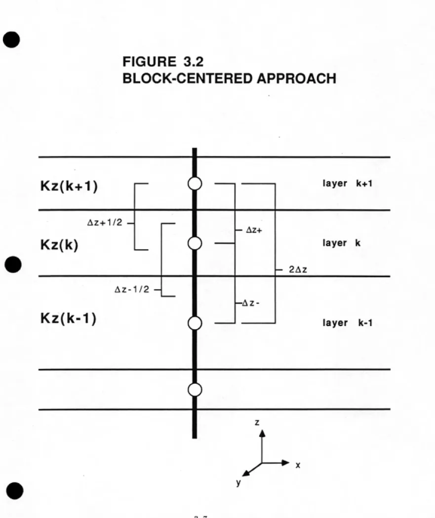
A finite difference approximation is applied to the z-derivative terms of (3.5), using

a central difference, block-centered approach. The block-centered approach refers to the

location of the nodes in the finite difference approximation and is illustrated in Figure

3.2. By using a block-centered approach, discontinuities in hydraulic conductivity can be

treated by taking a harmonic mean of the conductivity divided by the layer thickness. This

approach reduces the z-derivative terms to

§-M)-lMt^'^'

dz \ ^ Az_{\ n=l}

N

n=l

r^ I fen,k+l - fen.kA y- /^n,k-^n,k-l

Az_^Az J V Az-Az

where

indices k -h |,k — /rocl2,k -|-1, and k — 1 are as shown in Figure 3.2

Az terms are as shown in Figure 3.2 (L)

Kz+ = upper-weighted, harmonic-mean hydraulic conductivity [LjT) Kz- — lower-weigh ted, harmonic-mean hydraulic conductivity {LjT)

and harmonic mean is defined as Kz — ^„'^ ,,. where

d = total thickness [L)

d\ = thickness of individual layer (L)

K\ — hydraulic conductivity in indivdual layer [LjT)

FIGURE 3.2

BLOCK-CENTERED APPROACH

Kz(k+1)

i

layer k+1

Az+1/2

-r

Kz(k)

C

|) —

- 2Az Az1/2

-1

-Az-Kz(k-I)

S —J

X^AT,

n = l N

EiVn

n = l

K,^

K.

^n,k+l ~ fcn,k

if. ^n,k ~ ^n,k-l

A2_A2

A2+A2

hnk + 1

^^jJff^H- "

ͣ

n=l A2;+A2 A2_A2

/ln,k (3.7)

N

+ E^"

n=l

if.

Az-A^

^ii,k-The next step is to approximate the temporal derivatives using finite differences. An

Applying this approximation yields

dh dh d N _{hl^^ - h\}

dt dt dt -^ ^ ^ ^^ dt ^ ^ At

n=l n=l n=l

(3.8)

where

1 — index for present time step 1 + 1 = index for next time step

At = time increment for time step [T)

The remaining derivative terms can be expressed as follows

* N N

dh dh d v—v ,^ . , , v^ , , V

dx dx dx

n=l n=l

dx (3.9)

- N N

dh dh d \-^ ^r , t ^ v^ . / \

^ ^ ^ n=l n=l

dN^

dy (3.10)

By time-lagging the z-component terms, the original set of n^j, by n^ terms are split

into Tiz subsets of equations, each of which contains rixy equations. Time-lagging the

z-component terms implies that these terms are evaluated at the old (1) time step, while

the other components are evaluated at the new (1+1) timestep. The resulting equations

of head at the new (1+1) timestep, and the second representing the corrected approximate

values of head at the new (1+1) timestep. Splitting the equations in this manner allows

for computations in the x-y plane to be separated from computations for the z-direction,

thus easing the computational burden.

Instead of explicitly writing all terms of the two equations, they can be represented in matrix form as

iKHuwr''+^ ic^vr^' - Ch}i)

:{f(/.)}i'+^)* + {Fmi;-''^' + {KL . h)[_, - [{KU + KL)

ͣ

h]i + {KU

ͣ

h)i^.

and

[if^].wr^^'+^(wr^-{MO

={f (/.)}!'+')' + {F(/.)}i'+^)* + {KL

ͣ

h)it\ - [{KU + KL) . h)i+' + {KU • h)il\

(3.12) where

index * refers to predicted solutions and

[{h}('-^^) ~ {hy) = Sf N,S.^ dx dy

At

{T{h)}= ff N;T{h) dxdy

R.

{m}^^N;(Knl^) dB

{KL

ͣ

h)k-i - [{KU + KL)

ͣ

h]k + [KU

ͣ

h)k+i = JJ Nif, (if.g) dx dy

The model considered in this paper utilizes linear triangular elements in the x-y plane, as shown in Figure 3.3. The basis functions for this type of element are as follows.

^ni = ^[(2;n,yn„ - Xn,^yn^) + (yn, " ynJ\X + (x„„ - Xn^)y\

Ki = -^[{^nr^Vni - XmVnJ + (yn„ " yni)x + (x„, - Xn^)y]

^^"^ " ^[(^'i.^''. - ^n,yn,) + {yrti ' ynj)x + (Xn, - Xn,)y] (3.37)

where

ni,nj, and Um = nodal indices on triangular element

Xi,Xj,Xm,yi,yj, and t/m = coordinates of triangle vertices (L) Ae = area of triangle {L'^)

These basis functions are substituted into Equations 3.11 and 3.12 and subsequently

differentiated and integrated.

FIGURE 3.3

LINEAR TRIANGULAR ELEMENT

I

ͣ

JD "' (xi.yi)

/

o

\

j/^

\

^i.^^^^^

\

nj "^ ^

^^^...^^^^^

\

(xj,yj)

•

"^^^

^ nm

computational procedure. The first step is to lump-diagonalize the [ST] matrix, which

contains the storage terms, and the [KU], [KU+KL], and [KL] matrices, which contain the

vertical flow terms. The algorithm used to himp-diagonalize is as follows.

an = 2_^^i3 ' '^iy — ^ for i # j (3.13)

j where

fltj = i,j element of [A] matrix

This approach greatly simplifles the computation of the two equations (3.11 and 3.12).

[A] do not differ signifcantly over the nodes of a single element. The set of equations in

(3.11) can be termed the predictor equations.

The flrst stage of the solution procedure amounts to a layer-by-layer solution of the

predictor equations for h^^'^^^*. After the sublayer-sweeping operation has been completed,

the second stage of the algorithm is achieved by solving Equation 3.12 for h^^'^^\ the

corrective version of the flow equation. It is apparent that there are several terms in

(3.11) that are identical to those in (3.12). There is no need to solve the entirety of both

equations. The repeated terms can be eliminated by taking the difference of (3.11) and

(3.12), thus obtaining

= {KL • h)it\ - [{KU + KL) . h][+' + {KU • h)i\\ (3-14)

-{KL

ͣ

h)i_, + {{KU + KL) • h)i - {KU • h)[+,

The overall coefficient matrix on the right-hand-side of Equation 3.14 can be made

and [KL] are lump-diagonalized. A highly efficient tridiagonal solver such as the Thomas

Algorithm can be used to solve (3.14). The second stage of the computational procedure

thus involves solving rixy subsets of equations, with each subset containing n^ equations

with ng unknowns. The resulting solutions for h^''^^' are the current hydraulic head values

at the nodes on a vertical line along the complete thickness of the aquifer domain.

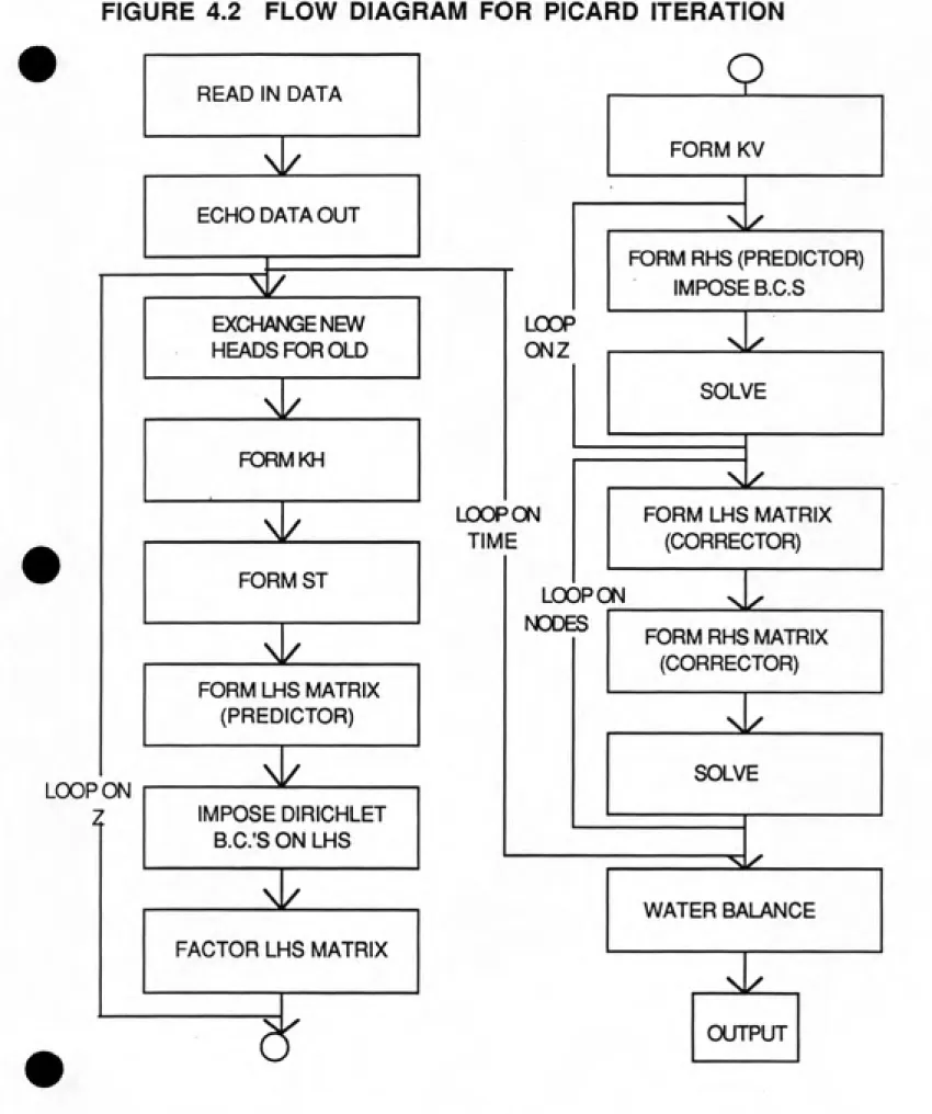
The computational procedure for setting up and solving the predictor and corrector

equations is summarized in Figure 3.4. The procedure is repeated for each time step until

the maximum number of timesteps (specified by the user) is reached. No iterations within

the timestep are necessary for the confined flow case, because direct solution procedures

are used.

3.3 Application of Boundary Conditions and Source and Sink Terms

Suitable boundary conditions and source or sink terms can be applied to the ALALS

algorithm. The most commonly applied boundary conditions for groundwater flow prob¬

lems are the Neumann or Dirichlet boundary conditions. Typical boundary conditions and

sources or sinks are shown in Figure 3.5.

The Neumann boundary condition can be generalized as

du{x,y,x,t)

dn

= g{x,y,z,t) (3.15)

B

where

n = outward normal vector

B = problem boundary

g = arbitrary boundary function

LOOP ONZ

FIGURE 3.4

FLOW DIAGRAM FOR ALALS ALGORITHM

READ IN DATA

.NJ^

ECHO DATA OUT

FORMKH

2^

FORM ST

jvk

FORM LHS MATRIX

(PREDICTOR)

^

IMPOSE DIRICHLET

B.C.'S ON LHS

Nk

FACTOR LHS MATRIX

jsk:

EXCHANGE NEW HEADS FOR OLD

W

2.

LOOP ONZ

FORM RHS (PREDICTOR),

IMPOSE B.C.S

Vj^

SOLVE

LOOP ON

TIME

Si^

FORM LHS MATRIX

(CORRECTOR)

LOOP ON NODK

nL^

FORM RHS MATRIX

(CORRECTOR)

^

SOLVE

WATER BALANCE

N^

FIGURE 3.5

TYPICAL BOUNDARY CONDITIONS,

SOURCES AND SINKS FOR

GROUNDWATER FLOW

RECHARGE

r^i

BOUNDARY

RJUX

CONSTANT HEAD BOUNDARY

NO FLOW BCO^DARY

by simply placing the free edge of an element on the relevant boundary. In the z-direction,

no flow conditions are imposed by setting the relevant portion of the the vertical flow

component equal to zero (see Equation 3.11). For example, at the top layer of an aquifer

system, the condition of no flow onto the top reduces the expression for vertical flow

components from Equation 3.11 as follows.

//

_{m£ (^^Ij I dxdy= (KL}

ͣ

_{/i)^_i - \{KU + KL)}

ͣ

_{h)[ (3.16)}

Fluxes into boundary elements can be applied in all three dimensions by integrating

the flux over the relevant element and applying the resultant to the nodes of the element.

The hydrologic quantity of recharge is an example of a boundary flux that may be applied

in groundwater flow. The integration is analogous to the boundary term found in Equation

3.5. Recharge can be handled as follows

11TM

dx dy = recharge (3.17)

R

where

Fr = recharge rate {L/T)

Dirichlet boundary conditions can be generalized as

UB (x, y, z, t) = f{x, y, z, t) (3.18)

where