1237.pdf

(1)

ABSTRACT

NANCY B. JONES. The Use of EPA's Currently Recommended

Default Concentrations as Initial and Boundary Conditions In

the Urban Airshed Model. (Under the Direction of Dr. Harvey

E. Jeffries).

EPA's list of recommended default concentrations, from the Guideline for Regulatory Application of the Urban Airshed Model, were substituted for SAI's AIRQUALITY, BOUNDARY, and

TOP CONC files In the Atlanta 5-cltles PLANR approach study.

These concentrations were also substituted for the ROM

(Regional Oxidant Model) derived AIRQUALITY, BOUNDARY and TOP CONC files in the ROM/UAM interface test case for the New York domain.

In the case of Atlanta, where the differences between the

original and default values were small, the peak

concentrations each hour were within a few ppb of each other

and domain-wide there were only changes of 10 to 15 ppb in the

concentration contours. However, both runs miss the peak

measured concentration by one-half.

The default input concentrations were usually less than

half of the ROM derived ones in the New York domain. Here

there is a large decrease in the model output of ozone, up to 80 ppb near the southern boundary and 50 to 60 ppb in the area of maximum concentrations. Even with these large decreases,

the difference between the UAM/ROM output concentrations and

the observed ozone concentrations are greater than the

difference between the UAM/ROM and the default run forecast

(2)

ABSTRACT...i i

TABLE OF CONTENTS...iii

ACKNOWLEDGEMENTS...v

LIST OF TABLES AND FIGURES...vl

1. INTRODUCTION AND BACKGROUND...1

1.1 INTRODUCTION...1

1.1.1 MAGNITUDE OF THE U.S. OZONE NON-ATTAINMENT PROBLEM...1

1.1.2 CHEMICAL AND PHYSICAL PROCESSES IN OZONE FORMATION...4

1. 2 PHOTOCHEMICAL MODELS...4

1.2.1 BACKGROUND...4

1.2.2 URBAN AIRSHED MODEL (UAM)...6

1.2.3 REGIONAL OXIDANT MODEL (ROM)...10

1, 3 UAM APPLICATIONS...12

1.3.1 PLANR APPROACH IN ATLANTA...12

1.3.2 UAM/ROM INTERFACE FOR NY DOMAIN...18

1.3.3 DEFAULT VALUES FOR INITIAL AND BOUNDARY CONDITIONS...25

2. PURPOSE AND APPROACH...27

2 . 1 PURPOSE...27

2 . 2 APPROACH...27

3. RESULTS...28

3 .1 ATLANTA...28

3 . 2 NEW YORK...39

4. DISCUSSION...62

4 . 1 FINDINGS...64

(3)

XV

REFERENCES...67

APPENDIX A: ATLANTA...Al

LIST OF TABLES AND FIGURES...A2

APPENDIX B: NEW YORK...81

(4)

I would like to thank Dr. Harvey E. Jeffries for his

encouragement, technical assistance and guidance during my study at the Department of Environmental Sciences and Engineering. I would also like to thank Dr. Donald L. Fox and

Dr. David Leith for their reading, listening and assistance.

Thanks also go to Carey Ji-Cheng Chang and Gerald R.

Gibson, without whom the UAM would not have run, making this work impossible; and to everyone in rooms 119 and 120 who've

listened to and helped me. Thanks go to Dr. James M.

Godowich, for his suggestions and help in obtaining data

files.

I especially would like to thank my husband Philip for

his encouragement and his help filling my prior role; and

Lauren and Adam for helping to raise each other and their not

so quiet acceptance of another day exceeding the National

Academy of Pediatrics recommendation for television viewing by

(5)

LIST OF TABLES AND FIGURES vx

TABLES

Table 1. Classified Ozone Non-Attainment Areas...3

Table 2 . Uam Input Files...9

Table 3. Observations Available for PLANR Study...14

Table 4. Default Concentrations from EPA Reg. Guide...25

Table 5. Default Concentrations as Input into Model...26

FIGURES Fig. 1. Fig. 2. Fig. 3. Fig. 4. Fig. 5. Fig. 6. Fig. 7. Fig. 8. Fig. 9. Fig. 10 Fig. 11 Fig. 12 Fig. 13 Fig. 14 Fig. 15 Fig. 16 Fig. 17 Fig. 18 Fig. 19 Fig. 20 1988 Population Above NAAQS...2

VOC/NOX/O3 Total Daily Cycle...5

Atmospheric Processes Treated in a Column of Grid Cells...7

UAM Simulation Program Input & Output...8

The ROMNET Domain for the Northeast...10

ROM Layer Characterization...11

UAM Domain for Atlanta...13

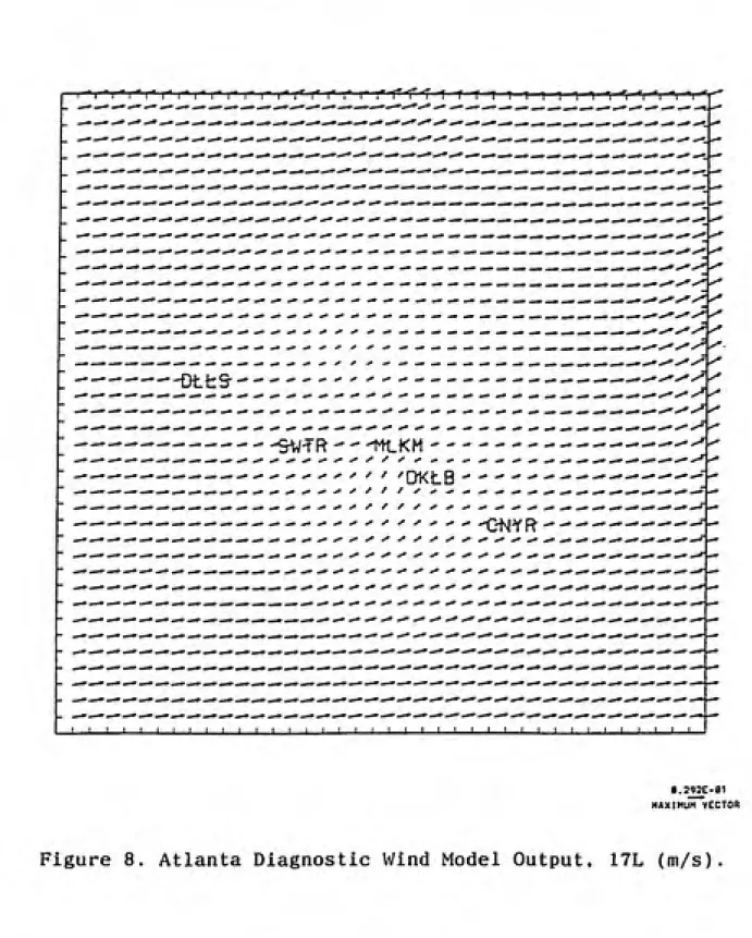
Atlanta Diagnostic Wind Model Output, 17L...16

Atlanta Original Ozone Contours, 17L..., . . 17

Flow Chart for ROM/UAM...19

New York Domain...20

Day 1, UAM/ROM Derived Winds, 17L...21

Day 1, UAM/ROM Ozone Contours, 17L...22

Day 2, UAM/ROM Derived Winds, 17L...23

Day 2, UAM/ROM Ozone Contours, 17L...24

Atlanta Initial Cond. 5-Cities Vs. Default...29

Atlanta Boundary Cond. 5-Cities Vs. Default...30

Atlanta Top Cone. 5-Cities Vs. Default...31

Atlanta Default Ozone Contours, 17L...32

(6)

Fig. 21. Conyers Observed Vs. Predicted Ozone...35

Fig. 22. Dekalb Observed Vs. Predicted Ozone...36

Fig. 23. Atlanta Ozone Frequency Dist. by Cell...37

Fig. 24. Atlanta Ozone Culm. Percen. Freq. Dist. by Cell...38

Fig. 25. NY Initial Cond. UAM/ROM Vs. Default...40

Fig. 26. NY Top Cone. UAM/ROM Vs. Default...41

Fig. 27. NY Boundary Cond. UAM/ROM Vs. Default,

NOx/Oj, West, Lev 1&2...42

NOX/O3, West, Lev 3,4&5...43

Fig. 29. NY Boundary Cond. UAM/ROM Vs. Default, VOC/CO, West, Lev 1&2...44

Fig. 30. NY Boundary Cond. UAM/ROM Vs. Default, VOC/CO, West, Lev 3,4&5...45

NOX/O3, South, Lev 1&2...46

NOX/O3, South, Lev 3,4&5...47

Fig. 33. NY Boundary Cond. UAM/ROM Vs. Default, VOC/CO, South, Lev 1&2...48

VOC/CO, South, Lev 3,4&5...49

Fig. 35. NY Default Ozone Contours, Day 1 17L...52

Fig. 36. NY Default Ozone Contours, Day 2 17L...53

Fig. 37. NY Change in Ozone Contours, Day 1 17L...54

Fig. 38. NY Change in Ozone Contours, Day 2 17L...55

Fig. 39. Hampstead Observed Vs . Predicted Ozone...56

Fig. 40. Middleton Observed Vs. Predicted Ozone...57

Fig . 41. Day 1, Observed 15L Ozone Cone...58

Fig. 42. Day 2, Observed 15L Ozone Cone...59

Fig. 43. NY Ozone Frequency Dist. by Cell...60

(7)

1. INTRODUCTION AND BACKGROUND

1.1 INTRODUCTION

1.1.1 MAGNITUDE OF THE U.S. OZONE NON-ATTAINMENT PROBLEM

Since the passage of the initial Clean Air Act (CAA) ,

much progress has been made in reducing the levels of all of

the criteria pollutants, except ozone. Despite a 1979

relaxing of the standard from 0.08 to 0.12 parts per million

(ppm), (taking one hour averaged concentrations, the expected

number of days per year with a daily maximum ozone level above

0.12 ppm must not be more than one) 98 areas in the United

States were classified as non-attainment in ozone by the

Environmental Protection Agency (EPA) in 1991 (See Table 1).

[EPA,1991b] It is estimated that one half of the population

of the United States lives in areas which are not in

compliance with the current standard, while it is still

debated whether that standard is a safe limit from a public

health viewpoint. In 1989, the relaxed standard was only

supported by one half of the members of the Ozone

Subcommittee, of the Clean Air Scientific Advisory Committee

to the EPA. The remainder of the members recommended a

reduced upper limit. [Lippraan, 1989]

For the latest year that statistics are available, 1988,

(8)

standard exceeded (Fig. 1).[EPA.1988] High levels of ozone in

the atmosphere are known to cause adverse human health effects

ranging from transitory respiratory changes to structural

changes in the lung. Crop damage and degradation of materials

are also results of high levels of ozone.

For those non-attainment areas classified as serious and

above, and also for interstate moderate areas (See Table 1),

the 1990 Clean Air Act Ammendments (CAAA) requires the use of

"photochemical Grid models" to demonstrate prospected

attainment. The EPA has interpreted this to mean the UAM,

unless equivalency can be shown.

People in counties with 1988 air quality above

primary National Ambient Air Quality Standards.

pollutant PM10 S02 CO N02 Ozone Lead AnyNAAQS 1 9

r \

b" ^

1'"

r \

l:,:™^f:!^::;ͣ:s;SSBSJ:fSWs::J:::! ;t.:^ ^ 1 20 40 60 80

millions of people

100 120 140

Figure 1. 1988 Population Above NAAQS.

Of the people affected by air quality above the

(9)

Table 1. Classified Ozone Non-Attainment Areas.

Listed by classification. (Source: EPA. 1991b)

Extrtm* • Los Angolss-South Coast Air Basin, CA

Chicago-Gaiy-Laka County, IL-IN Houston-GaKrsston-Brazoria, TX

MilwaukM-Racina, Wl

Baltimors, MD

Phiiadslphia-Wnm-Trent, PA-NJ-OE-MD

Atlanta, GA

Baton flouga, LA

Beaumont-Port Arthur, TX

Boston-LawrancA-Worcester (E.MA), MA-NH

a Paso, TX Groatsr Connacticut

Muskogon, Ml Atlantic City, NJ

Charisston, WV

Chartotts-Gastonia, NO CIncinnati-Haniiiton, OH-KY Claveland-Akron-Lorain, OH Dallas-fort Worth, TX

Oayton-Springfiald, OH

Oatroit-Ann Arbor, Ml Grand Rapids, Ml

GrMnsboro-Wlnston Salam-H Point, NC Huntington-Ashland, WV-KY

Kawaune* Co, Wl Knox & Lincoln Cos, ME Lewiston-Aubum, ME

Louisvilla, KY-IN

Manitowoc Co, Wl

Albany-Schenactady-Troy. NY

Allentown-Bathlaham-Easton, PA-NJ

Altoona, PA

Birmingham, AL

Buffalo-Niagara Falls, NY Canton. OH

Cherokaa Co, SO

Columbus, OH Door Co, Wl

Edmonson Co, KY

Efia, PA

Essax Co (Whitafaca Mtn). NY Evansvilla, IN

Greanbriar Co, WV Hancock & Waldo Cos. ME Harrisburg-Lsbanon-Cartisla, PA Indianapolis. IN

Jafferson Co, NY Jersay Co, IL

Johnsto\wn. PA

Kent and Queen Anna's Cos, MO

Area Ozone design value Deadline

Classification (parts per million) Marginal .121 up to .138 Moderate .138 up to.160 Serious .160 up to .180 Severe .180 up to .280 Extreme .280 and above

New York-N New Jer-tong Is, NY-NJ-GT

Southeast Oasart ModHIad AQMA, CA

S»nn-13

Serious

Modarata

San Olago, CA

Ventura Co, CA

I

Portsmouth-Oover-Rochester, NH ProvManca (Alt RQ. R>

Sacramento Metro, CA

San Joequin Valley, CA

Sheboygan, Wl

Springfield (Western MA), MA Washington, OC-MO-VA

Mlami^bft Lauderdala-W. Palm Beach, FL

Monterey Bay, CA

NashvUle,TN

Parkaraburg. WV

Phoarac AZ

Pittsburgh-Baavar Valley, PA Portland, ME

Raleigh-Ourtiam, NC Readkig. PA

Richmond-Petersburg, VA

Salt Lake City, UT

San Frandsco-Bay Area, CA

Santa Bari>ani-Santa Maria-Lompoc, CA St Louis. MO-IL

Toledo, OH

MarginMl

Knoxviie, TN Lake Chartas, LA Lancaster, PA

Laxington-Fayatta, KY

Manchester, NH

MemfMs, TN

Norfoik-Vlr. Beach-Newport News, VA Owensboro, KY

Paducah. KY

Portland-Vancouver AQMA, OR-WA Poughkaepsie, NY

Reno. NV

Scranton-Wilkas-Barra, PA Seattla-Tacoma, WA

Smyth Co, VA (White Top Mtn)

South Bend-EIkhart IN

Sussex Co, OE

Tampa-St. Patarsburg-Clearwatar, FL

Walworth Co, Wl

York, PA

Youngstown-Warren-Sharon. OH-PA

(SubMatginai Kansas City. MO-KS)

3 years after enactment 6 years after enactment

9 years after enactment

(10)

The formation of ozone near the earth's surface peaks

during the summer months when the incoming solar radiation is

strongest. Coupled with the more intense radiation and

resulting increase in photolysis of ozone precursors, is the

retreat northward of the polar frontal boundary in the summer.

As a result there is an increased frequency of capping high

pressure conditions, where the vertical dilution of pollutants

is supressed. These conditions in turn allow emissions to

build up into large concentrations of primary pollutants.

Figure 2 shows the cycle of volatile organic carbons

(VOC) and NOx (all nitrogen species), in the lowest level of

a 20 Km grid cell from the Regional Acid Deposition Model

(RADM) . OH radicals react with VOC and are recreated in a

cycle. The cyclic process oxidizes NO to NO^ and the NO2

photolizes to reproduce the NO and to produce ozone.

1.2 PHOTOCHEMICAL MODELS

1.2.1 BACKGROUND

Photochemical models are mathematical descriptions of

atmospheric transport, diffusion, and chemical reactions of

pollutants. Their input data characterizes the emissions,

topography and meteorology of the region, while their output

describes the regions air quality. [NAS,1992]

The principal use of air quality models is to predict

future compliance with standards after planned emission

reductions. To confidently predict the results of these

planned reductions, the ability of the model to replicate past

(11)

r ^ (T)

H-< OQ l_j 1-5 O CO ' I ft) ?r 3 < O o n w X ^^ H- O ri- H cr o ft

rt-> •2 *< . '< n .-^ h-' C_ fD

S "J

QfQ o

- n

New York cilv area (20 km) 3.96 OH Cycles

34.1 ppb new OH

propagalioi) and Icnniiialioii

PoH=0.747

AVOC= 112.9ppbV 135.1 ppb OH

13.18 ppb by organics : ^^^^^^^ (N0-^N02 ) / VOC

20.92 ppb by inorganics;

= 1.84

48.1 ppb from emiss.

0.4 ppb lost by met

47.9 ppb new NO

N0-^N02 = 208.2 ppb (N0->N02) / NO,

210.1 ppb NO

reacted

---ͨ

100.9 ppb OH

re-created

[Q3]p/[N02]p

5.76 ANO,= 36.17ppbV

Pno=0-772

propagation and termination

0.709

162.3 ppb NO

re-created

---ͨ

[03]p=147.6ppb

4.39 NO Cycles

63.8 ppb [Oali™,

5.9 ppb [OaUct „ 65.6 ppb [O3]

met

[O3], =139.9 ppb

(12)

empirical kinetic modeling approach (EKMA) was the model

required by EPA for use in attainment demonstrations. EKMA is

a simpler trajectory model in which a "box" is moved along,

expanded and contracted by the meteorological conditions,

while passing over sources the emissions are added, and the

chemical reactions occur as the "box" moves. This model may

still be acceptable to EPA in some moderate non-attainment

areas.

Grid based (Eulerian) models use a three-dimensional

set of cells in which the species are passed from cell to cell

according to the meteorological conditions. The choice of the

dimensions of the grid cells implies that input data (winds,

turbulence, emissions, etc.) are resolved to that scale. [NAS,

1992]

1.2.2 URBAN AIRSHED MODEL (UAM)

The basis for the UAM is the atmospheric diffusion or

species continuity equation.

d/dt(c) + ud/dx(c) + vd/dy(c) + wd/dz(c) - D{dVdx^(c) +

dVdy^(c) + dVdz^(c)} = S - L (where d is the partial deriv)

( or Dispersion - Molecular Diffusion = Sources - losses)

The system of partial differential equations describes the

production of ozone and other species by expressing them as a

function of: advection, turbulent diffusion, chemical reactions, emissions and sinks such as surface deposition.

The solution of the coupled mass balance equation provides a

time dependent concentration of the species in the model. For

each three to eight minute time interval, for each grid cell,

the model solves the mass balance equations using the method

(13)

These are:

Step 1-solve advection/diffusion in the x-direction;

Step 2-solve advection/diffusion in the y-direction;

Step 3-add emissions & solve vertical advection/diffusion;

Step 4-perform chemical transformation of pollutants.

T Tnupom 2 TmipeR a 8

1

Tnmtpon Elavaad Twpipott Bsviud I I Tfipott tlBBlpOH Graoi^-Uvill

Ro«4w«y Mif wh Effi

INVE]ISDNTOP

TnnipoR

DfVBUIONBASB

. GROUND SUKFACE

I to 10 HlwMin »j

Figure 3. Atmospheric Processes Treated in a Column of Grid Cells. (Source: EPA, 1990b)

The kinetics mechanism for the chemical transformation of

pollutants in the latest version of the UAM is the Carbon Bond Mechanism IV (CBM-IV). Due to computational constraints, the mechanisms of ozone formation in the atmosphere can not be

expressed explicitly. In CBM-IV, reactive species are lumped

into surrogate groupings with similar kinetic characteristics.

The UAM uses up to thirteen input files, and outputs three files. (See Figure 4 & Table 2) Two episodes were

modeled for this report which had previously been set up and

which came with the UAM tapes as test cases. As a result time

(14)

Boundary Cond. Rxn Rates Control

[ diffbr£ak[

( regionrop ( ( emissions (

(tb>iperatok(

TEIWAIN

(opooral)

PTSOORCH ( ( AKQUALITYC

(boundary^

( TOPCONC {

(cHEMPARAMf (SD

SMCOmXOL

UAM

.^ SinuUdaa

-/ INSTAKr* ( f AVERACB f f DEPOSTIKJuf

Instant can be used as an initial condition file to

restart model.

Figure 4. UAM Simulation Program Input and Output Files

(15)

Table 2. UAM Input Files. (Source: U.S.EPA, 1990b)

AIRQUAUTY This file specifies the initial concentrations for each of the CB-IV state species (see Table 2-1) in each grid cell at the start of the

simulation.

BOUNDARY This file contains the locations of the modeling domain boundaries

and the concentrations of each species used as boundary conditions along each lateral boundary for each level,

CHEMPARAM This file contains information on the chemical species to be simula¬

ted, including reaction rate constants, upper and lower bounds,

activation energy, reference temperature, and resistance to surface

sinks.

OtFFBREAK This file specifies the daytime mixing height and nighttime inver¬

sion height for each column of cells at the beginning and end of

each hour of the simulation.

EMISSIONS This file specifies the ground-level emissions of all emitted species

to be simulated for each grid cell and each hour of the simulation. These species will usually be a subset of those listed in Table 2-1,

although any additional species not recognized by UAM will simply be ignored by the UAM.

METSCALARS This file contains hourly values of meteorological parameters that do not vary spatially. These scalars are the NO2 photolysis rate

constant, the concentration of water vapor, the temperature

gradient above and below the diffusion break, the atmospheric pres¬

sure, and the exposure class (a measure of the near ground-level atmospheric stability due to surface heating or cooling).

PTSOURCE This file contains point source information, including the stack

height, temperature, flow rate, the plume rise (effective stack height). Che grid ceil that contains the stack, and emission rates for

all emitted CB-IV species for each point source for each hour of the

simulation.

RECIONTOP This file specifies the height above ground of the top of the model¬

ing regioru It can vary both spatially and temporally, but the usual

practice is to set it to a constant.

SIMCONTROL This file contains simulation control information, including the

period of simulation, model options, and information on integration time steps.

TEMPERATUR This file specifies the surface temperature for each hour and grid

ceU.

TERRAIN This file contains values for surface roughness and deposition factor

(or each grid cell.

TOPCONC This file specifies the concentration of each CB-IV state species

(Table 2-1) (or the area above the top of the modeling domain.

VINO This file specifies the x- and y-direction components of wind

velocity for every grid cell for each hour of the simulation. Also

contained in this file are the maximum wind speeds (or the entire

domain and the average wind speed at each boundary (or each hour

(16)

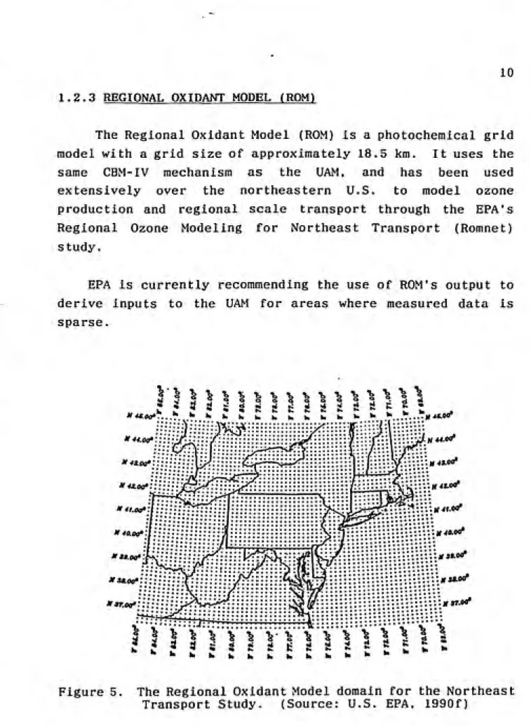
1.2.3 REGIONAL OXIDANT MODEL (ROM)

The Regional Oxidant Model (ROM) is a photochemical grid model with a grid size of approximately 18.5 km. It uses the same CBM-IV mechanism as the UAM, and has been used extensively over the northeastern U.S. to model ozone production and regional scale transport through the EPA's Regional Ozone Modeling for Northeast Transport (Romnet)

study.

EPA is currently recommending the use of ROM's output to derive inputs to the UAM for areas where measured data is

sparse.

•b -k "k \

t> W h. k. hi k.

'\'\'\W\\

s c ^

Figure 5. The Regional Oxidant Model domain for the Northeast

(17)

11

In the ROM, for the horizontal component of the mass

continuity equation is solved over the 19 km grid to determine

the transport. The vertical resolution is coarse and uses a

lower resolution, layer-averaged wind field to save

computation time.

The model takes into account the effects of cumulus

clouds on vertical transport, nighttime wind shear and

tubulence associated with the nocturnal jet, and terrain

influenced motions. Originally written as a four layer model,

the ROM-2.1 does not use the surface layer.

Layer Functions 0«vliiiM Layer 3 Layer 2 Layer 1 Layer 0

Oownward Iramport of llraloipherle oiona

Upward IrinipofI by

aimului cloudl

3. Liquid and gai phai*

pholochamlilry

4. Long rang* trampert

by fiaa •tmotphtra

1. Gat pliata phelochamitliy

2. Turbulenc* aitd wind ihear

adacli on lianiport and

dilluilon

3. Oepoiillon on mounlalni

4. Laka and marina layart

' 1. Eflecl on reaelion rala of

nibgriil icala legragalion of fraih and aged polluiani* 2. Qround dtpoiilion

3. Spatial variation in mean

concenttalioni ihie to lina

point and aiaa loiMcai

Figure 6. Regional Oxidant Model Layer Characterization.

(18)

1.3 UAM APPLICATIONS

The UAM has been exercised successfully using specially

derived data bases obtained from field studies. In these

cases, the model has performed well, resulting in the EPA's recommending its use by the states in the attainment demonstrations required by the CAA.

1.3.1 PLANE APPROACH IN ATLANTA

In the raid-eighties, EPA contracted with Systems Applications International (SAI) to demonstrate the low-cost

application of the UAM in five cities, using what was called

the PLANR approach. That is, SAI used National Weather

Service meteorological data, routinely measured ozone

observations, and the 1985 NAPAP emissions inventory, instead

of conducting the special field program that had been used in past applications.

The prepared computer files for one of these cities, Atlanta, is included on the UAM program tapes received from EPA, and is the "original" Atlanta simulation referred to in this paper. The simulation begins on 1200L June 3, 1984 and simulates the high ozone episode of June 4, 1984. The domain

consists of a 40X40 array of 4km grid cells.

The wind fields were created using the Diagnostic Wind

Model (DWM), supplied as part of the UAM distribution, to

obtain 14 vertical levels of winds. These were then averaged

to the UAM 5-layer structure, and adjusted to eliminate

vertical velocity through the top.

An hourly wind field is created in two steps. First, a

(19)

13

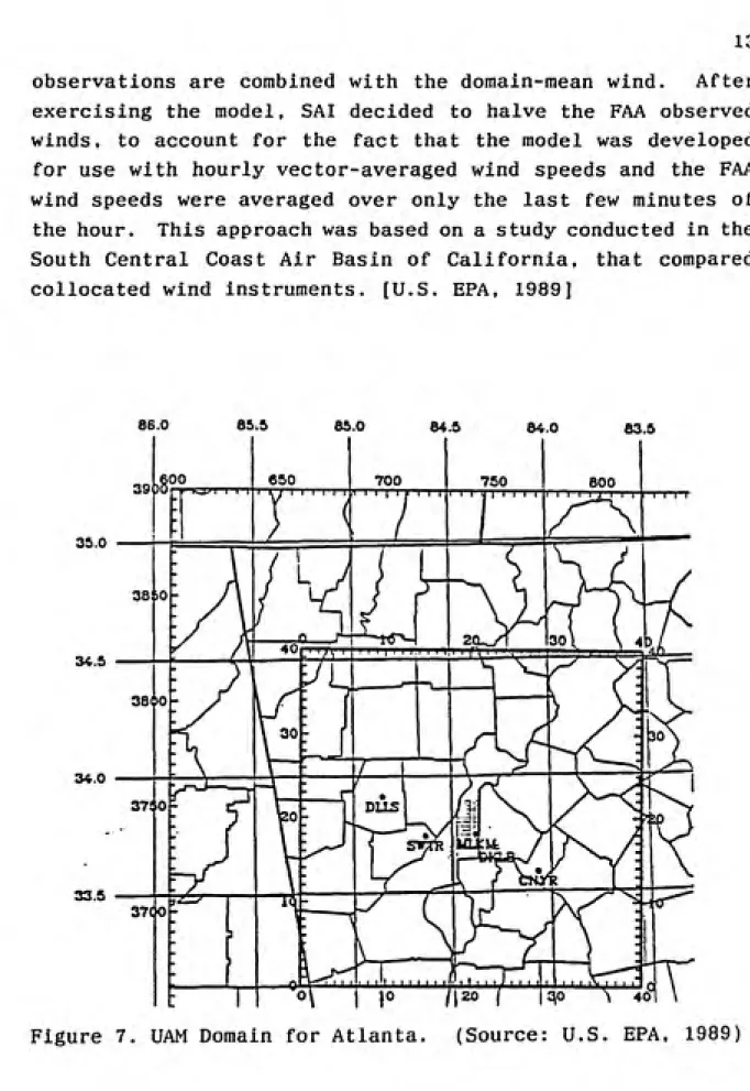
observations are combined with the domain-mean wind. After

exercising the model, SAI decided to halve the FAA observed

winds, to account for the fact that the model was developed

for use with hourly vector-averaged wind speeds and the FAA wind speeds were averaged over only the last few minutes of

the hour. This approach was based on a study conducted in the South Central Coast Air Basin of California, that compared

collocated wind instruments. [U.S. EPA, 1989]

86.0 es.s 85.0 84.5 S4.0 83.5

35.0

34.5

34.0

33.5

5

381 »0

(20)

Table 3. Observations Available for PLANR Study. (Source:

U.S. EPA, 1989)

Surface observations and data available:

wind speed (WS), wind direction (WD), temperature (T), dewpoint temperature (TD) and pressure (P).

Site Name

Location UTMX

UTM (Zone 16)

UTMY Variables Measured

Atlanta Hartsfield

International Airport 739.580 3726.148 WS, WD, T, _{Td. p}

Dobbins Naval Air Station 729.590 3755.498 WS, WD, T, _{Td- p}

Fulton County (Charlie

Brown) Airport 729.9^7 3740.709 WS, WD, T, _^D Dekalb Peachtree Airport 749.7214 3752.306 WS, WD, T, _Td Conyers Monastery Monitor 772.248 3719.869 WS. WD

South Dekalb Panthersville

Monitor 752.780 3730.991 WS, WD, T, _h

Upper-air observation sites, locations, and distance from Atlanta used in this study.

Location UTM Coordinate

UTMX

839.644

s (Zone 16)

UTMY

Dj At

stance fro:

Site Name Ut

35°

Lon;^

57' 83° 19'

-lanta (ks)

Athens, GA 3763.429 109

Nashville, TN 36° 15' 86° 34' 538.182 4012.482 199

Greensboro, NC 36° 5' 79° 57' 1134.426 4016.946 U91

Wayeross, GA 31° 15' 82° 24' 937.394 3467.152 328

Centerville-Brent AL 32° 54- 87° 15' 475.841 3640.638 275

Ozone monitor names and locations.

UTM Location (Zone 16)

Monitor JD Monitor Name UTMX UTMY

(21)

15

In the Atlanta study, for the initial concentrations,

boundary conditions and top concentration input, SAI used the following values:

VOC 25 ppbc(using EKMA default speciation)

Isoprene 0.0001 ppb

NOx 1 ppb (75:25 N02:N0) Ozone 40 ppb

CO 200 ppb.

In the Atlanta Study, maximum ozone concentration in

excess of 150 ppb was predicted by the model however, it was

well north of the Conyers Monastery (CNYR) where a daily

maximum of 145 ppb was recorded. For more information about

(22)

r I' I" r r r rT' r r r -r r f"r<'''\ t t t t t i i t i -i -i -^i ͣ I i I (

•-fDttS---•--- ' ' 'DKtB

ON^R

J_____I_____\_____I_____I_____1_____I_____I_____1_____I_____I_____I I I_____I_____1_____I_____\---1_____I_____I_____I---1---1---1---1_____I_____\_____I_____I_____i_____I_____I_____I_____I_____i---L.

HAXIMUH VECTOR

(23)

17

-1—I—I—I—I—1—I—I—I—I—I—I—I—r "1—I—:—I—1—I—I—I—I—I—I—I—I—I—r

80

&0

41 .8

(24)

1.3.2 UAM/ROM INTERFACE FOR NEW YORK DOMAIN

As a portion of the ROMNET study for the northeast, the

EPA contracted with Computer Sciences Corporation (CSC) to

develop an interface system between the ROM model and the

smaller scale UAM. Thus, for cities where routine

meteorological and air quality data are scarce and funds are

not available for large scale studies, the ROM model output

can be accessed for use as input into the UAM. While

temporally the Interface is straightforward, since both models

use one-hour resolution steps, there are spatial framework

differences in the models.

Horizontally the UAM is based on a cartesian coordinate

system with a finer grid spacing (generally 2 to 8 kilometers)

and a smaller domain (around 200 kilometers). Conversely, the

ROM is based on a latitude-longitude system, with a horizontal

resolution of 1/4 degrees longitude and 1/6 degrees latitude

(approximately 19 kilometers at midlatitudes) and the domain

is about 1000 kilometers. In the UAM, the vertical diffusion

break is the key in marking the separation of layers of cells

above and below the mixing height, however, the ROM model has

no emulation for the diurnally-varying diffusion break height.

In the ROM/UAM interface, the horizontal wind fields are

matched from ROM's layer 1 to the two lowest layers of the

UAM, and ROM's layer 2 to the three upper layers.

There are seven interface programs. Four produce input

files for the UAM preprocessors, and the other three produce

binary files for use directly in the UAM program. Figure 9

Indicates which files are replaced by the output files of the

(25)

en c

n

en o i— o d-o

C (T> C

o h« o

ft a cr

•• OR p

CWrl-CO W o

rr "5

mm

>• o

"v.

•- C to > co 2

o

URBAN AIRSHED MODELING SYSTEM

IdXKT I

c a

uwrr 1 |w>na| jtrwm. Tvntn u_ rwawc 1—. ͣ NDAIT

|Dinno«le Wind Mode 1

1 •

h _rr

L -j

i •

' 1

• tUHVNC 1 1

111

Emiiiloru PnpncttHr Syitcm m

^]

rmia i___ NOTE:

(*) indiatei processor b replaced by ROM/UAM Interface

(1) domain iptdfic ((drain and chemistrj)

(2) episode specific

(3) growth factors can be applied

(4) control factors can be applied

IUU J

1 »

DUfUT UAMrn

(26)

Interfacing is performed for initial, boundary, and top

concentrations of 17 of the 23 pollutant species in the UAM CB-IV. For the other 6 species (NXOY, CRES, MGLY, OPEN, PNA,

and ETOH), values are determined by the steady-state,

lower-bounds values in the CHEMPARAM file. Non-ROM derived input,

such as winds or concentrations, can also be used together with the ROM input. Finally the UAM/ROM interface does not provide emissions, simulation control or chemistry parameters

input to the UAM.

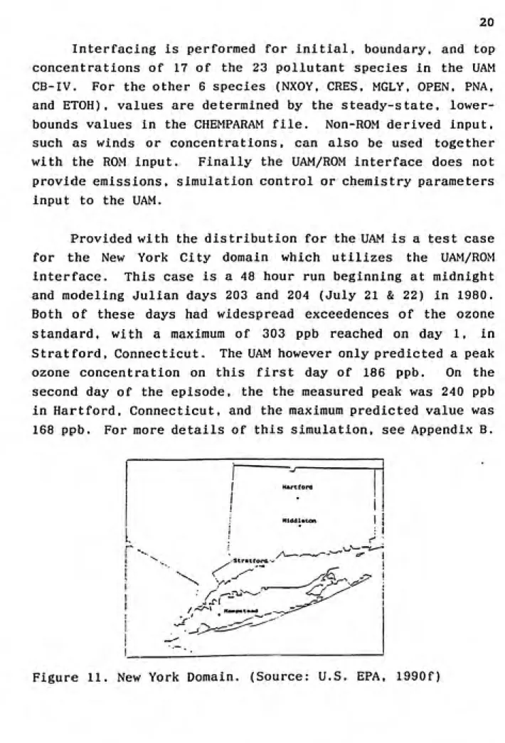
Provided with the distribution for the UAM is a test case for the New York City domain which utilizes the UAM/ROM interface. This case is a 48 hour run beginning at midnight and modeling Julian days 203 and 204 (July 21 & 22) in 1980. Both of these days had widespread exceedences of the ozone standard, with a maximum of 303 ppb reached on day 1, in Stratford, Connecticut. The UAM however only predicted a peak ozone concentration on this first day of 186 ppb. On the second day of the episode, the the measured peak was 240 ppb in Hartford, Connecticut, and the maximum predicted value was 168 ppb. For more details of this simulation, see Appendix B.

(27)

21

l\

i ]

_{\ \}

_\

_{M \ ^ M M \ \ \}

\ \ \ \ \ \ \ \ \

J

1 '

_{1 i i}

_i

t \ \ \ \ \ V \ \ \ V

\ \ \ \ \ \ \ \ J1 \ 1 1 1 I T" 1 1

^ ^

_{\ \ \ \ \ Vf^ \ \ nAa}

\ \ \ \ \ 1 \ 1 J

t 1

_{t t M M \\ V ^ ^^ \ \ \ \ \ t t 1 J}

[ 1 f ^

! 1 t 1 t 1 -A \ \ \ J>\\ \ \ \ \ \ \ \ J

f

1 ^ ^

_{fff!1\<\\\^\\\\N\\\J}

}

i A A

f t 1 1 \ \ \)\ \y7^ ^ Y \ N \ \ \ N J

'f

t 4 <

/ / / / f f m \ \it/\ \ \ \ \ \ \ \ J

~f f f f

/ / / / / f t\t \ ^ vV/mC^ "^ "^ ^ ^ "^ "^

f ' f f

/ / f / f / 1 [ \ \ V 0,0/v.^ X \ \ \ \ ^J

-

r f M 1 ^ V V---A

^ ^ ^'^ N \ \ N ^J

. ' III t

\ \ \ \ \ N ^ i. ,_ ..-.-»-

.-^vjx \ \ \ \ -J

1 _•

\ \ \ \ N •»-. ._'^L..,__.,,__ͣ<__ͣ*-

.-^N^AN \ \ \ -J

< «

\ \ \ -v^^^^JV.^^-

.v,\iY \ \ V J

^ ^

r

\

r

N V ^_ ,_\ N \/\ \ \ \\\\ N V N>^

^

- r \

\v,-._______.V\>e]\\\ ^\\ ^ ^ "J

^j

_r^r-\-\-

\-

-— /\- .\ \C^ \ N \H ^ N ^|

'i

. \ \ \ \

N V...\ V \^\L> "^ ^V

L \ \ ^^

^l- \ \ N \

N s V...^^"^^X^^"^ "^ I

, \ \ ^

\- \ \ \ \

N N N V... -^^"^ YA ^ M

\|

. \ \ \ \

V V V V...^'

ͣ

"^^ H ^ iJ

\j- \ \ \ \

\ \ \ \ V > . . ./. ' / Pft^v-O-I 1 y~\

\i. \ N \ \

\\\\\v.../'^// »!<|/r\ / /t J

v^

. \ \ \ \

\\\\\\>.y.///// /""-O/ / ^ -I

^J

. N \ N \

\ \ \ \ \ \ ,,/.///// / /T / i

\. \ \ \ \

\\\\\\x/. /-////////}

\. \ \ \ \

\ \ \ \ \ \ v/ . 1 f ^ /////// 1

r]- \ \ \ \

\\\\\\/v^.if///////|

\ N N N \ \ \ \ \ \./r(\ \)\tittff///v

m 1

(28)

^

(29)

I 1 1! M 11 IJ I I M

i \t -M-V 23

Ai

\ V.v \ \ \ \ \ \ \ \ \ \ \ \ \ \ \ \ \ \ \ \ \ \\\\\\\\ \\\\\\\N

N N N N \ Vv,^ N \ N N N^^-.

V. N NN Nv. v.^.

\ \

\ \ N N

Xl X

N.

N \\\ \ \/

\ \/\ \ \

"s N W »>. ""N V. \ \ \

V V. ^N \

N1^ \ \ \\

\ \ \ \ V

v|.\ \ \ \ \ \\NV^^VVN

N\\\\\NV«s.»s.^xN\

^NW^^^v^vN \ \ )( \ \ \ \

k'sv^'v.^v.vn n n y\ s n s \

.VV.v^v^vVNNX \/\ \ \ \ \ \

^ V. V, V, v. v, \. v. N.-Vrrv \. \ \, \ \ \

\ \ \ \ \

\

A

\ \ \ S \ \

\ \ \ \

N \ \ \ \ \ N

\ \ \ \ \ \ N

N \ \ \ \ \ N

\ \ ^ \ \ \ ^

(30)

HtM \

^^

(31)

ͣ

-^

25

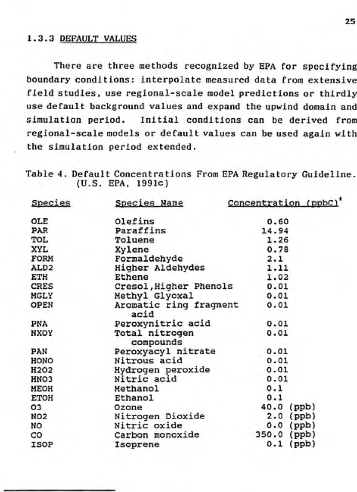
1.3.3 DEFAULT VALUES

There are three methods recognized by EPA for specifying

boundary conditions: interpolate measured data from extensive

field studies, use regional-scale model predictions or thirdly

use default background values and expand the upwind domain and simulation period. Initial conditions can be derived from

regional-scale models or default values can be used again with

the simulation period extended.

Table 4. Default Concentrations From EPA Regulatory Guideline

(U.S. EPA, 1991c)

Species Species Name Co

OLE Olefins

PAR Paraffins

TOL Toluene

XYL _Xylene

FORM _Formaldehyde

ALD2 _{Higher Aldehydes}

ETH Ethene

CRES _{Cresol,Higher Phenols}

MGLY _{Methyl Glyoxal}

OPEN _{Aromatic ring fragment}

acid

PNA _{Peroxynitric acid}

NXOY _{Total nitrogen}

compounds

PAN _{Peroxyacyl nitrate}

HONO Nitrous acid

H202 _{Hydrogen peroxide}

HN03 Nitric acid

MEOH Methanol

ETOH Ethanol

03 Ozone

N02 _{Nitrogen Dioxide}

NO Nitric oxide

CO Carbon monoxide

ISOP _Isoprene

Concentration fpobcV

0.60 14.94 1.26 0. 2, 1. 1. 0, 78 1 11 02 01 0.01 0.01 0.01 0.01 0, 0, 0, 0. 0, 0. 40. 2, 0, 350, 0, 01 01 01 01 1 1 0 0 0 0 1 (PPb) (ppb) (ppb) (ppb) (ppb)

(32)

4

Currently EPA is recommending that, whenever feasible, the UAM/ROM Interface System be used to derive initial and boundary conditions. Further, they recommend that the winds

from the interface system also be used to prevent

inconsistencies in mass fluxes passing through the domain. If

the area to be modeled is not within the ROM domain and if

measured data are not adequate, then they recommend that the

default values in Table 4 be used. [U.S. EPA, 1991cJ

Some errors exist in Table 4 as printed by the EPA, Table

5 contains the default concentrations as input into the

simulations, after clarification from EPA and the creators of the CB-IV mechanism.

Table 5. Default Concentrations as Input into Model DEFAULT VALUES

AIRQUALITY, BOUNDARY & TOP CONC

CONC. PPM _CONC.(PP

SPECIES C #

NO O.OOE+00 O.OOE+00

N02 2.00E-03 2.00E+00

03 4.00E-02 4.00E+01

ETH 5.10E-04 2 1.02E+00 OLE 3.00E-04 2 6.00E-01 PAR 1.49E-02 1 1.49E+01 TOL 1.80E-04 7 1.26E+00 XYL 9.75E-05 8 7.80E-01 FORM 2.10E-03 1 2.10E+00 ALD2 5.55E-04 2 l.llE+00 ORES 1.43E-06 7 l.OOE-02 MGLY 3.00E-06 3 9.00E-03 OPEN 2.00E-06 5 l.OOE-02

PNA l.OOE-05 l.OOE-02

NXOY l.OOE-05 l.OOE-02

PAN l.OOE-05 1 l.OOE-02 MEOH l.OOE-04 1 l.OOE-01 ETOH 5.00E-05 2 l.OOE-01

I SOP l.OOE-04 l.OOE-01

CO 3.50E-01 1 3.50E+02

HONO l.OOE-05 l.OOE-02

H202 l.OOE-05 l.OOE-02

(33)

2. PURPOSE AND APPROACH

2.1 PURPOSE

The purposes of this project were: 1) to learn to operate

the UAM, its preprocessors, and the NCAR (National Center for

Atmospheric Research) Graphics programs; 2) to conduct a

sensitivity analysis of ozone predictions to initial and

boundary conditions. In this study, EPA's table of default

concentrations (Table 4) , were substituted for SAI-derived

inputs for an Atlanta scenario and for EPA's UAM/ROM Interface

predicted values for a New York scenario.

2.2 APPROACH

The two test cases which accompany the UAM code were

rerun using the concentrations recommended by EPA as default

values. Table 4 contains the list of default boundary

conditions as recommended for use by the EPA, and used to

replace the AIRQUALITY, BOUNDARY and TOPCONC files in both the

Atlanta and the New York simulations. Some questions were

raised about the concentrations listed in table 4, such as

lumped species carbon numbers, necessary for conversion from

ppbc to the required ppm input to the model. Table 5 contains

the concentrations as input into the simulations, after

clarification from EPA and creators of the CB-IV mechanism.

It is necessary to mention again that, the wind field is

adjusted so that the vertical velocity through the top is

zero. Thus no interchange takes place across the region top,

(34)

3.1 ATLANTA

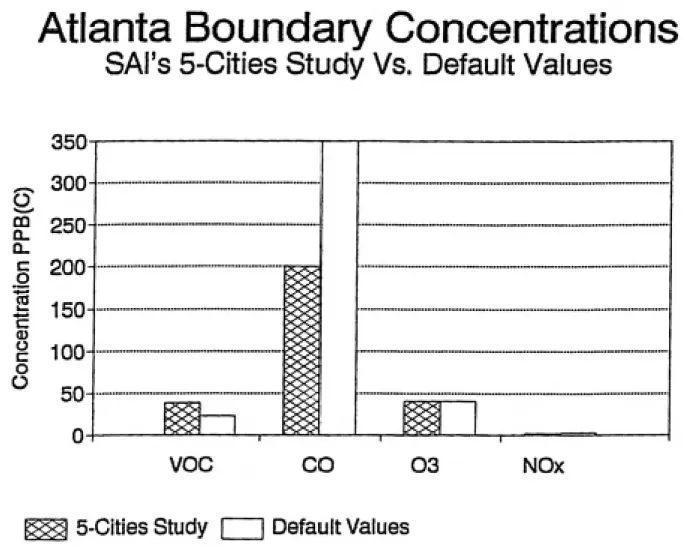
Figures 16, 17 and 18 contrast the inputs to the three

files where the default values were substituted for the input

derived by SAI. In this instance, there is very little

difference between the initial and boundary conditions, with the exception of the much increased amounts of CO in the

default simulation. Appendix A contains tables presenting the

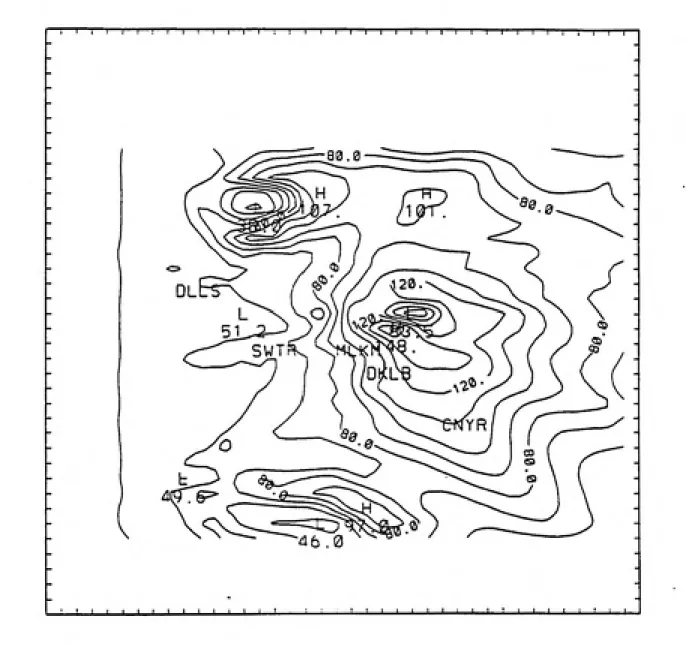
concentrations depicted in the graphs in greater detail.

The interesting result is how little change was made in

the output of the model. The maximum concentration of 148 ppb

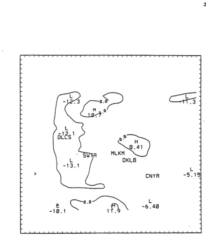
at 17L (Figure 19), was nearly identical to the 150 ppb

originally forecast. Figure 20 shows the results of

subtracting the cell by cell concentration of the default

output from the concentrations derived originally. Upwind of

the city the large area of negative contours reflect the

default run forecasting approximately 20% greater

concentrations of ozone formed. The areas where the run

original forecast higher values are all correlated with point

sources of NOX.

(35)

29

Atlanta Initial Air Quality Cone.

SAI's 5-Cities Study Vs. Default Values

350 300

g

g 250

I 200

I 150

c

(D

^

100-o

" 50

fs^^n

M

i

^

voc CO 03 NOX

^ 5-Cities Lev. 1&2 ^ 5-Citles 3,4&5

Default Values

(36)

Atlanta Boundary Concentrations

SAI's 5-Cities Study Vs. Default Values

350

_ 3004

O

g 250

I 150

c 0)

B

100-o

^

50-voc CO 03 NOx

5-Cities Study | | Default Values

(37)

31

Atlanta Top Concentration

SAI's 5-Cities Study Vs. Default Values

350

300-O

^ 250

1 200

I 150

c

^ 100

o

^ 50

VOC CO 03 NOx

5-Cities Values I I Default Values

(38)

T—I—I—I—!—I—I—r T---1---1---1---1---1---!---1---1---\---!---1---1---1---!---r

S0

~dt .<2

_i_______I_______I_______I_______I---1---1---1---\---1---L. _;_______I_______I_______I_______I______I______i_______1_______I_______1_______1_______I______I_______I_______I_______L.

(39)

33

1—I—I—I—r "1—1—I—I—\—]—1—]—[—r

MLKM

DKLB

10.1

0.a

CNYR

L

•6.40

L

ͣ

5. 151

_i_______I_______I I I I I I_______I_______I_______I_______I_______I—i—1_ I

I___I_II_)_I_I_I_I_I_I_____i-Figure 20. Atlanta Change in Ozone Contours, 17L (ppb).

(40)

concentration at the Conyers site at night, (the graph begins at midnight, 12 hours after the simulation had begun). Both runs miss the peak concentration at the Conyers site by one-half, and seriously underestimate the concentration throughout

the afternoon hours. At the Dekalb site, the model runs come

much closer to predicting the afternoon concentrations, with

a timing error begun as early as 9 a.m. being the dominant

feature.

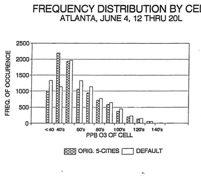
A cell by cell frequency distribution comparison of the two runs concentrations was done, with the results are shown

in Figures 23 and 24. Four cells were deleted from the north,

west, and south sides for this comparison, because when SAI

originally made their study a decision was made to reduce the domain size. This also explains the blank areas of the wind and contour diagrams. This analysis shows that the original

(41)

35

OBSERVED VS. PREDICTED VALUES

CONYERS MONASTERY

150 m z o N o m Q-100 50-n ͤ ͤ ͤ n ͤ

n n ͤ ͤ ͤ ͤ ͤ

1---1---i---1---r

4

1---1---1---1---r

12

8 12 16

HOURS (FIRST 12 OMITTED)

\-,. n -1---1---1---1---r 20 ͤ MEASURED---S-CITIES DEFAULT

Figure 21. Conyers Observed Vs. Predicted Ozone.

(42)

OBSERVED VS. PREDICTED VALUES

DEKALB JR. COLLEGE

150

m 100

O M O m

CL a.

50

ͤ

HOURS (FIRST 12 OMITTED)

ͤ

MEASURED---5-CITIES

DEFAULT

(43)

37

FREQUENCY DISTRIBUTION BY CELL

ATLANTA, JUNE 4, 12 THRU 20L

2500

LU

z 2000

111

cc

O 1500-O

O

LU

az

u.

1000-500

04

<40 40's

ffla-i

r-a-i

60's ao's IOCS 120's

PPB03 0FCELL

140's

ORIG. 5-CITIES DEFAULT

(44)

FREQUENCY DISTRIBUTION BY CELL

ATLANTA, JUNE 4, 12 THRU 20L

C/)

100 o

U- 80

O

LU

O 60

<

h-ͣz.

LU

o 40

oc

LU

Q-20

d 0

—I---1---1---1---1---1---i---1---1---1---1---1---r

40 60 80 100 120 140 160

PPB 03 OF CELL

ORIG. 5-CITIES -- DEFAULT

Figure 24. Atlanta Ozone Culmulative Percentage Frequency

(45)

39

3.2 NEW YORK

The New York domain is very different than the Atlanta

one. Large amounts of ozone and its precursors are transported into the region. Only CO is increased when

substituting the default concentrations for the ROM derived

ones. At 350 ppbC the default CO is consistently higher than the ROM value. Otherwise, the ROM derived input is generally twice the default values. Figures 25 through 34 track the initial air quality condition, and the boundary conditions at

the upwind sides of the domain for the first 24 hours of the

simulation. Again the TOP CONC default file is only included

for consistency and has no effect on the outcome of the

simulation.

Unlike Atlanta, varying the Initial and boundary conditions did have a profound effect upon the outcome of the

simulation (Figures 35 & 36). The area of maximum concentrations occured in the same region for both the UAM/ROM

run and the default value run, roughly along the Connecticut coast, in the same area where the peak observations were.

However, on the first day the area of greatest change In forecast ozone concentration was along the southern boundary, where the default input ozone concentration was less than half

the ROM value. Figure 37 shows the first day difference, with the default concentrations subtracted from the UAM/ROM ones.

There is nearly a linear progression in the decrease of the

concentration difference as one progresses northward,

(46)

N.Y. Initial Air Quality Cone.

ROM Derived Vs. Default Values

350

^ 3004

O

^ 250

I 200

I 1504

(U

^ 1004

o

^ 50

^

voc CO 03 NOx

UAM/ROM Lev. 1&2 ^ UAM/ROM 3,4&5

Default Values

(47)

41

N.Y. Top Concentration File Input

ROM Derived* Vs. Default Values

350

^ 300^

O

g° 250

I 150

c <u

^ 100

o

O

50

P^?^

voc CO 03 NOx

ROM Derived Values I I Default Values

"^Average of first 24 hrs.

(48)

125

CQ

CL Q_

C

o

15

0)

o

c

o

O

100-75

50-

25-0

N.Y. Boundary Conditions

ROM Derived Vs. Default Values

West Edge, Levels 1&2

UAM/ROM 03

Default 03

UAM/ROM NOx

.Default NQx.

—1---1---1---1---r-2 4 6

—1 I---1 I---1---i---1---1---1---1---;---i---1---1---1—

8 10 12 14 16 18 20 22

Time in hours (first 24 hrs.)

24

Figure 27. New York Boundary Conditions UAM/ROM Vs. Default

(49)

43

125

CQ

Q-C

q

ͣ

(3

c

0)

o c

O

100

75i

50-25H

N.Y. Boundary Conditions

ROM Derived Vs. Default Values

West Edge, Levels 3,4&5

UAM/ROM 03

Default OS

UAM/ROM NOx .Default.NQx

0~'~T---1---1---1---1---1---\---1---1---1---i---'---1---1 1---1---1---1---1---1---1 T

2 4 6 8 10 12 14 16 18 20 22 24

Time in hours (first 24 hrs.)

Figure 28. New York Boundary Conditions UAM/ROM Vs. Default.

(50)

N.Y. Boundary Conditions

ROM Derived Vs. Default Values

400-

350-WestEdge,

Levels 1&2

Default CO

o CD CL

300-^

250-c

O

c

200-

150-'^^'^^___________

UAM/ROM CO^..--^''';'^

0)

o

1

o

O

100-^----^x^

5

0-\.^__

UAM/ROM VOC..-^^ 1

——--__ ^..^.-^'^''^ 1

-I----1----1----1----1----1----1----1----1----1----1----1----1----i----1

'^°^^°|mt|V>f'^|----1----1----1—r-2 4 6 8 10 1'^°^^°|mt|V>f'^|----1----1----1—r-2 14 16 18 '^°^^°|mt|V>f'^|----1----1----1—r-20 '^°^^°|mt|V>f'^|----1----1----1—r-2'^°^^°|mt|V>f'^|----1----1----1—r-2 '^°^^°|mt|V>f'^|----1----1----1—r-24

Time in hours (first 24 lirs.)

Figure 29. New York Boundary Conditions UAM/ROM Vs. Default

(51)

45

400

350-o 300

m

n

Q- 250

c

o

ͣ

55 200

1^

+-• c 0)

o 150

c

O

100 50

N.Y. Boundary Conditions

ROM Derived Vs. Default Values

West Edge, Levels 3,4,&5

Default CO

UAM/ROM CO

JJAM/ROMVOC.

Time in hours (first 24 hrs.)

T—I—!—I—I—I—[—I—I—;—I—I—I—I—I r r " r ~i i—i—i—i—r^

2 4 6 8 10 12 14 16 18 20 22 24

(52)

125

OQ

CL

Q-C

o

C

0)

o c

o o

100

75-

50-

25-N.Y. Boundary Conditions

ROM Derived Vs. Default Values

South Edge, Levels 1&2

UAM/ROM 03

Default 03

UAM/ROM NOx

Default NOx

—I---1---1---1---1---1---1---1---1---1---1---1---1---1---1---1---1---1---1---1---1---1---r

2 4 6 8 10 12 14 16 18 20 22 24

Time in hours (first 24 hrs.)

(53)

47

N.Y. Boundary Conditions

ROM Derived Vs. Default Values

125

CQ

Q-Q. C o

o

c

o o

100-

75-50

25-South Edge, Lev6ls3,4&5

UAM/ROM 03

Default 03

UAM/ROMjNjOx^

Default NOx

0~^---1---1---1---1---1---1---1---1---1---1---1---1---1---1---1---1---1---1---1---1---!---T"

2 4 6 8 10 12 14 16 18 20 22 24

Time in hours (first 24 hrs.)

Figure 32. New York Boundary Conditions UAM/ROM Vs. Default

(54)

N.Y. Boundary Conditions

ROM Derived Vs. Default Values

400

South Edge, Levels 1&2

350

o 300

CQ

Q-CL 250

c

o

B 200

u. c

o 150 c

o O

100

50-Default CO

UAM/ROM CO

UAM/ROM VOC

DefaultVOC'

T---1---1---1---1---1---1---;---1---1---1---1---1---1---i---1---1---1---1---1---1---1---1 I

2 4 6 8 10 12 14 16 18 20 22 24

Time in hours (first 24 hrs.)

Figure 33. New York Boundary Conditions UAM/ROM Vs. Default

(55)

400 350

^ 300

m

§: 250

c

ͣͣ

§ 200

§ 150

c

^ 100

50-N.Y. Boundary Conditions

ROM Derived Vs. Default Values

South Edge, Levels 3,4&5

Default CO

UAM/ROM CO

UAM/ROM VOC

Default VOC

49

Time in hours (first 24 hrs.)

"1 I I---1 I I i I 1 i i ~i I I I I i I 1 I r

2 4 6 8 10 12 14 16 18 20 22 24

(56)

On the second day of the simulation, a day where observed concentrations were much lower, the pattern of the change in

forecast ozone was much different. Here there was not the

zonal variation which reflected the decrease of each boundary from its earlier value, rather the change was greatest at the center of the domain and over New York City itself (Figure

38).

For the comparison of observations to 4 nearest cell

forecast concentrations, Hampstead, Long Island and Middleton,

Connecticut were chosen (See Figure 11). These locations were chosen because they were some distance inland, and so less likely to be influenced by difficult to model land-sea

breezes, and because they were somewhat in the center of the

domain and so less likely to be influenced by the boundary condition variation. The comparisons begin at noon on the first day, 12 hours after the beginning of the simulation, and

continue until sunset on the second day.

Hampstead (Figure 39) reflects a near center city

location, less likely to have variations caused by transport errors. Although the UAM/ROM simulation misses both days peaks, and is slower to decrease after the peak is reached, it

does an adequate job of modeling the diurnal variations. The default run underestimates the observed concentration

throughout most of the time period, however its lack of accuracy is not so very different than that of SAI's 5-cities run for Atlanta which they considered a success (Figures 21 &

22) .

For Middleton, which is near the center of the domain, and far enough inland to be away from the land-sea breeze effect, the model performance was much worse. Here we see less of a difference between the UAM/ROM and default run's

(57)

51

both afternoons. A look at the wind vectors forecast by the

ROM in Appendix B, shows that for much of the day a westerly

component of the wind was predicted for this region, this

would advect relatively clean air from the Catskill region of

New York over the region. The ozone observations suggest that

the urban plume was blown in a northeasterly direction

directly over central Connecticut (Figures 41 & 42).

A cell by cell frequency distribution of concentrations shows that the default run produces an excess of cells with concentrations below 70 ppb and very few above 150 ppb. The UAH/ROM output produces a more normal distribution (Figure 43)

(58)

-I---1---\---\---r-%^

I I_________' I ' '_________I_________I_________L. -J________1________' I I________L.

(59)

53

a®

_ 4

-i_____\_____l_l___L_J_____L. _l_____I_____I_____l_ _l_____I_____i_____L.

(60)

34 .8

Figure 37, New York Change in Ozone Contours. Day 1 17L (ppb)

(61)

55

40 .0

©

Figure 38. New York Change in Ozone Contours, Day 2 17L (ppb)

(62)

OBSERVED VS. PREDICTED VALUES

HAMPSTEAD. NY

300

250-LU

200-n'

O 150

\n ͤ °

HOURS (FIRST 12 OMITTED)

ͤ

MEASURED---UAM/ROM

DEFAULT

Figure 39. Hampstead Observed Vs. Predicted Ozone.

(63)

57

OBSERVED VS. PREDICTED VALUES

MIDDLETON, CT

300

250

d

150-°

ͤ

E^Q-O-*"!—I—I—I—I—I—I—I—I—I—I—I—I—I—1—I—I—I—I—I—I—I—I—I—I—I—i—I—I—I—r 16 20 24 4 8 12 16 20

HOURS (FIRST 12 OMITTED)

ͤ

MEASURED---UAM/ROM ... DEFAULT

Figure 40. Middleton Observed Vs. Predicted Ozone.

(64)

Figure 41. Day 1, Observed 15L Ozone Concentrations. Daily

maximum for large portion of region. (Source:

(65)

59

Figure 42. Day 2, Observed 15L Ozone Concentrations. Daily

maximum for large portion of region. (Source:

(66)

FREQUENCY DISTRIBUTION BY CELL

NEW YORK, DAY 203, 12 THRU 20L

1200 O 1000

<40 40'S 60's 80's 100'S 12as IAD's ISO's ISO's

PPB 03 OF CELL

UAM/ROM DEFAULT

(67)

61

FREQUENCY DISTRIBUTION BY CELL

NEW YORK, DAY 203, 12 THRU 20L

C/5

100

LU

O

Ll_ 80

o

LU

o ₆₀

<

1-Z

LU

O 40

CC

LU CL

20 ^

_J

ID

O 0 t---1---r^—I---1---1---1---1---1---1---\---1---r 40 6,0 80 100 120 140 160

PPB 03 OF CELL

180

UAM/ROM -- DEFAULT

(68)

In their Regulatory Guide, EPA suggests the best case scenario for determining the initial and boundary conditions would be based on an intensive field program, with modeled

data filling in any gaps. While resources are seldom

available to obtain this type of data, and regional models do not provide complete coverage of the U.S., EPA has provided default concentrations. [U.S. EPA, 1991b] In this case the initial and boundary conditions were replaced with those

default concentrations, and the results are at times dramatic.

The two sets of input files were generated from different methods, Atlanta's input files being gathered from limited readily available air quality and meteorological data, while New York's was generated by the UAM/ROM interface. The two domains modeled were also very different, Atlanta is

surrounded by a large expanse of rural areas, presumably then clean background air is being transported into the domain. Also because of this, the default values which the EPA has

recommended are very close to the values selected by SAI in

the initial modeling. Conversely, New York is part of the larger eastern corridor, where ozone and precursors are not only being emitted into the domain, but also a large portion is transported in from upwind metropolitan areas. In this

case, the default input concentrations were often less than half of the ROM predicted ones. Thus we are able to compare

the results of the two extremes in variation of initial and

(69)

64

I do not attempt to address the appropriate use of

default values. In their Regulatory Guideline, EPA is very

clear that these values should be limited to areas surrounded

by large areas of low-density anthropogenis emissions, with an

extended domain, and in areas without regional transport of ozone and its precursors. This is a first step in the

sensitivity analysis which EPA recommends when the default values are used.[U.S. EPA, 1991bl

It is apparent that the Atlanta simulation fits the guidance criteria for use of the default values. However,

caution should be taken in assuming the validity of the input concentrations, and the lack of dependence of the output on the varied initial and boundary conditions. When these input

files were prepared for the original run, their values were determined in a similar manner. SAI assumed concentrations

which were generally accepted as reasonable background air values, and these have changed very little. A more powerful

test of the validity of these concentrations and the association between the initial and boundary conditions and model output, would be a comparison between use of the default

values and the use of measured values from an extensive field

study. Unfortunately these input files were not available, however this topic is covered in the 5-cities study in a

(70)

4.1 FINDINGS

Meteorological uncertainty has a greater impact on model

performance than variations in initial and boundary

conditions. When comparing model output to observed air

quality data, both the original 5-Clties and the UAM/ROM, and

their default runs, were a superior match at the near center

city locations (Figures 22 & 39), than at the corresponding

transport dependent locations (Figures 21 & 40) .

Secondly, in the case of Atlanta, while in both instances

the model predicts a peak concentration very close to the

observed, it is not near the location of this observation. This can be attributed to either an incorrect characterization

of the wind field, or to the prudent placement of monitors by

the regulated. The model consistently predicts a trough in

the ozone contours along the line of monitors in Atlanta,

without more complete monitor coverage, it is impossible to

seperate underprediction of concentrations throughout the

domain from transport errors.

Thirdly, in the New York simulations, there is a greater

discrepency between the observed concentrations (Figures 41 &

42) and the UAM/ROM predictions, then between the two

simulations (Figures 13, 15, 35-38 & Appendix B) . In this

case, as in the possibility of domain-wide underprediction in

Atlanta, the error may lie in the prediction of excess

dilution resulting from a too high mixing height. This mixing

height variation could be the true cause of the 303 ppb ozone

observation at the Coast Guard Lighthouse in Strattford, with

the pollutants trapped below the low-level inversion set up by

(71)

66

scale model (wind fields were generated from the ROM for this

application).

The impact of variations in initial and boundary

conditions is very real however, and the impact on model ozone

output increases proportionately with changes in the input concentrations. In Atlanta, where the deviation of the default inputs from the original is small, the change in the

model output is also small. Whereas in New York, where most of the inputs were reduced by half or more, the change in model ozone output is great. The change in output is in the range of 50 to 60 ppb throughout the areas of maximum forecast concentrations, during the afternoon hours. This would reflect the change in forecast locally produced ozone. Near the southern boundary, where the change in transported ozone

(72)

4.2 FURTHER WORK

Implicitly, two questions were discussed here: 1) how adequate are the default input concentrations for the initial and boundary files in various scenarios, and 2) what is the impact of changes in these initial and boundary conditions on

the final output ozone concentrations.

In the first case, a comparison of the use of default concentrations, to ROM derived ones, and measured ones from a

field study on the same episode would be the first choice. Secondly the New York domain could be worked with further by

varying the wind field to affect horizontal transport and the

vertical velocity dependent mixing height.

As an exercise in the effects of initial and boundary inputs to a model, both domains could be rerun with further variations in the input concentrations, either incremented as

(73)

67

REFERENCES

Air and Waste Management Association, 1988. "Ozone Control Strategies, The Scientific and Technical Issues Facing

Post-1987" . Transactions of an APCA International Speciality Conference. Air and Waste Management Association.

Gery, M., Personal Communication, May 1992.

Jang, J., "Sensitivity of Ozone to Model Grid Resolution", thesis presented to the Department of Environmental Science

and Engineering, at Chapel Hill, N.C., in 1992, in partial

fulfillment of the degree of Doctor of Philosophy.

Lippman, M. , 1989. "Health Effects of Ozone: A Critical Review", Journal of the Air and Waste Management Association, 39:672-695.

National Academy of Sciences, 1992. Rethinking the Ozone Problem in Urban and Regional Air Pollution, Washington, DC, National Academy Press.

Seinfeld, J.H., 1988. "Ozone Airquality Models: A Critical

Review", Journal of the Air Pollution Control Association, 38:616-645.

U.S. Environmental Protection Agency, 1982. "A Regional-Scale

(1000 Km) Model of Photochemical Air Pollution: Part 1, Theoretical Formulation", EPA-600/3-85-035, Office of Air

Quality Planning and Standards, Research Triangle Park, NC.

U.S. Environmental Protection Agency. 1989. "5-City Urban Airshed Model Study", Draft report. Office of Air Quality Planning and Standards, Research Triangle Park, NC.

U.S. Environmental"Protection Agency, 1990a. "National Air Quality and Emissions Trends Report", 1988, EPA-450/4-90-002. Office of Air Quality Planning and Standards, Research Triangle Park, NC.

U.S. Environmental Protection Agency, 1990b. "User's Guide for

the Urban Airshed Model, Volume I: User's Manual for UAM

(CB-IV)", EPA-450/4-90-007a, Office of Air Quality Planning and

(74)

U.S. Environmental Protection Agency, 1990c. "User's Guide for the Urban Airshed Model, Volume II: User's Manual for UAM

(CB-IV) Modeling System", EPA-450/4-90-007b, Office of Air Quality

Planning and Standards, Research Triangle Park, NC.

U.S. Environmental Protection Agency, 1990d. "User's Guide for the Urban Airshed Model, Volume III: User's Manual for the

Diagnostic Wind Model", EPA-450/4-90-007c, Office of Air Quality Planning and Standards, Research Triangle Park, NC. U.S. Environmental Protection Agency, 1990e. "User's Guide for

the Urban Airshed Model, Volume IV: User's Manual for the Emissions Preprocessor System", EPA-450/4-90-007d, Office of

Air Quality Planning and Standards, Research Triangle Park,

NC.

U.S. Environmental Protection Agency, 1990f. "User's Guide for the Urban Airshed Model, Volume V: Description and Operation of the ROM-UAM Interface Program System", EPA-450/4-90-007e, Office of Air Quality Planning and Standards, Research Triangle Park, NC.

U.S. Environmental Protection Agency, 1991a. "Regional Modeling for Northeast Transport (ROMNET)", EPA-450/4-9I-002a.

Office of Air Quality Planning and Standards, Research

Triangle Park, NC.

U.S. Environmental Protection Agency, 1991b. "Ozone and Carbon

Monoxide Areas Designated Nonattainment", EPA report. Office

of Air Quality Planning and Standards, Research Triangle

Park, NC.

U.S. Environmental Protection Agency, 1991c. "Guideline for

the Regulatory Application of the Urban Airshed Model", EPA-450/4-91-013 Office of Air Quality Planning and Standards,

(75)

(76)

LIST OF TABLES AND FIGURES