KyleOnda_MSPHFinal.pdf

(1)

INTERMITTENT VS. CONTINUOUS WATER SUPPLY: WHAT BENEFITS DO HOUSEHOLDS ACTUALLY RECEIVE? EVIDENCE FROM TWO CITIES IN INDIA

Kyle Steven Onda

A technical report submitted to the faculty of the University of North Carolina at Chapel Hill in partial fulfillment of the requirements for the degree of Master of Science in Public

Health in the Department of Environmental Sciences and Engineering.

Chapel Hill 2014

Approved By: Jamie Bartram

Meenu Tewari Pete Kolsky

i

(2)

(3)

ABSTRACT

Kyle S. Onda: Intermittent vs. Continuous Water Supply: What benefits do households actually receive? Evidence from two cities in India

(Under the direction of Jamie Bartram and Meenu Tewari)

(4)

(5)

ACKNOWLEDGEMENTS

This project would not have been possible without the support of many people. I am deeply thankful to my co-advisor Dr. Jamie Bartram, who has supported me throughout my research on many projects and has guided my development as a scholar. I also wish to express my gratitude to my co-advisor Dr. Meenu Tewari, who introduced me to this particular topic, and provided constant and essential guidance and encouragement through every phase of this project. I also heartily thank Pete Kolsky for serving on my committee.

I would also like to thank the department of Environmental Sciences and Engineering, The Water Institute, the department of City and Regional Planning and UNC Chapel Hill for providing a fantastic learning environment and experience. A special thanks to the International Association of Plumbing and Mechanical Officials and the Indian Council for International Economic Research, whose financial support made this project possible; Ruth David for her fieldwork support during my stay in Nagpur; Mme. Agarwal for her support during my stay in Amravati; the current and former officials at the Maharashtra Water and Sanitation Department, Nagpur Environmental Services Ltd., Orange City Water, and Maharashtra Jeevan Pradhikaran for their willingness to be part of the project. I also thank Andy Guinn for useful feedback on an earlier draft of this report.

(6)

LIST OF TABLES

Table 1 Potential impacts of continuous water supply . . . 15

Table 2 Comparison of Nagpur and Amravati water supplies, 2009-2013 . . . 24

Table 3 Probit regression for propensity scores based on observed household characteristics . . 27

Table 4 Observed covariates over continuous water supply treatment before and after Propensity Score Matching . . . 28

Table 5 The average effect of continuous water supply on water demand . . . 30

Table 6 Quantile difference-in-differences, effects of continuous water supply on lpcd . . . 31

Table 7 Quantile difference-in-differences with kernel propensity score weighting, effects of continuous water supply on lpcd . . . 32

Table 8 Reasons given by households with continuous water supply why they do not prefer continuous water supply . . . 47

Table 9 Amravati domestic water tariff structure . . . 61

Table 10 Nagpur domestic water tariff structure (non-slum) . . . 62

Table 11 Nagpur domestic water tariff structure (slum) . . . 62

Table 12 Reported coping behaviors for non-slum households . . . 63

(10)

LIST OF FIGURES

Figure 1 Location map of study sites . . . 9

Figure 2 Timeline of domestic billing record availability and CWS treatment group status for Amravati . . . 17

Figure 3 Median lpcd in Amravati domestic water connections, October-November 2009 to December-January 2013 (unweighted) . . . 26

Figure 4 Median lpcd in Amravati domestic water connections, October-November 2009 to December-January 2013 (weighted) . . . 29

Figure 5 Percentage of non-slum households exhibiting storage behaviors . . . 34

Figure 6 Percentage of slum households exhibiting storage behaviors . . . 35

Figure 7 Reasons given by households with continuous water supply using tanks why they still use tanks . . . 37

Figure 8 Percentage of non-slum households exhibiting treatment behaviors . . . 40

Figure 9 Percentage of slum households exhibiting treatment behaviors . . . 41

Figure 10 Percentage of non-slum households using alternate water sources . . . 42

Figure 11 Percentage of slum households using alternate water sources . . . 43

Figure 12 Preference of intermittent water supply households for continuous water supply (Nagpur) . . . 45

(11)

LIST OF ABBREVIATIONS

24x7 24 hours per day, 7 days per week CWS Continuous Water Supply

CPHEEO Central Public Health and Environmental Engineering Organization (Government of India) DMA District Meter Area

IBT Increasing Block Tariff IRB Institutional Review Board IWS Intermittent Water Supply

JNNURM Jawaharal Nehru National Urban Renewal Mission LPCD Liters per capita per day

MJP Maharashtra Jeeven Pradhikaran (State Water Board) MLD Million Liters per Day

NESL Nagpur Environmental Services Ltd. (Nagpur Water Regulator)

NRW Non-revenue Water

OCW Orange City Water (Nagpur Private Water Utility Operator) PSM Propensity Score Matching

SLB Service Level Benchmarks (Government of India) UNICEF United Nations Children’s Fund

(12)

1 Introduction

1.1 Background

Worldwide, 4.2% of deaths are attributable to deficiencies in water supply, sanitation, and hygiene practices (Prüss-Üstün et al.,2008). Thus, supplying safe water is a major priority for developing countries and international organizations. In 1990, 71% of the urban population in low and middle-income countries were estimated to have access to water piped to their house plot or inside the house. By 2010, estimated piped water coverage increased to 73%, meaning that new water connections generally kept pace with population growth (UNICEF and WHO,2012). Moreover, access to piped water does not by itself guarantee access to water that is safe, microbiologically or chemically clean, available in adequate quantities, or supplied reliably and predictably (Onda et al.,2012). A major reason for this discrepancy is intermittent supply of water, even when delivered through piped connections. The practice of non-continuous or intermittent water supply (IWS) (supplying water to the distribution system for less than 24 hours per day, every day) is widely recognized as a significant risk factor for drinking water contamination (Besner et al.,2011;EPA,2001; Karim et al.,2003;Lehtola et al.,2004;Telgmann et al.,2004), and for pressure transients that can damage

a water system over time (Lee and Schwab,2005). Intermittent supply is also a driver for costly coping mechanisms that in turn decrease service quality for other users. For instance, construction of storage tanks and operation of booster pumping mechanisms not only burden the implementing households directly in the form of time and monetary expenditure, but can lower service pressures and water quantity for other users and introduce further uncertainty in the hydraulics of the system, leading to inequitable distribution of water (Pattanayak et al.,2005;Lee and Schwab,2005). Estimates from international surveys of water utilities indicate that up to one third of Latin American and African water utilities, and the majority of water utilities in South Asia operate their networks intermittently (van den Berg and Danilenko,2011).

(13)

Nairobi, Kenya; Manila, Philippines; Dakar, Senegal; and the nation of Burkina Faso (Water and Sanitation Program-Africa,2009;Chiplunkar et al.,2012). They have made these efforts at considerable expense,

generally requiring capital expenditure grants and loans from central governments and/or international donors (Chiplunkar et al.,2012;Water and Sanitation Program-Africa,2009). Such expenditures for more recent CWS upgrades in India have been justified under the explicit assumption that the intervention will produce benefits to households in the form of better quality water, improved health, and lowered per capita expenditures on water storage, pumping, and treatment (World Bank,2010). However, does it follow that upgrading water supply from IWS to CWS will automatically ensure that customers will actually experience reductions in the adverse consequences of IWS? What does it take for the assumed benefits of 24x7 service hours? There is little evidence as to whether, under what conditions, and what categories of households actually receive the purported benefits of converting from intermittent to continuous water supply. This paper attempts to provide grounded primary evidence in the urban Indian context to begin to address this gap in the literature between assumptions of CWS supply and the realization of benefits by consumers.

This technical report is organized as follows: It reviews the debate on the merits of continuous water supply; then uses the terms of the debate to build the conceptual framework used to link continuous water supply to potential benefits for domestic consumers, and the research questions that guide the rest of the paper; follows with a description of the methods in terms of study sites, study design, and data collection and analysis; and concludes by analyzing the results in light of the existing literature on water service quality, discussing the policy implications of the findings, and providing perspectives on avenues for further research.

1.2 Converting from Intermittent to Continuous Water Supply: Debates in the Literature

This section provides a background of IWS and CWS and an overview of the debates in the literature about the merits of the introduction of CWS in a formerly IWS network. First, it explains common causes or motivations of IWS system operation. The main criticisms of IWS are outlined, and finally, it summarizes the purported benefits of CWS currently being used to justify large-scale interventions in Indian and international water policy and engineering fields.

1.2.1 Causes of Intermittent Water Supply

(14)

in varying degrees to drinking water contamination at the point of use as well as waterborne disease outbreaks (Geldreich,1996;Lee and Schwab,2005;Semenza et al., 1998). One commonly cited deficiency is the practice of intermittent water supply. Generally a water utility either adopts intermittent supply or passively lets its network degrade and operate intermittently due to a variety of constraints–of water availability, financial resources, managerial capacity, or all three (Lee and Schwab,2005). For instance, a utility may be compelled to provide intermittent water supply due to rapid population growth and a lack of concurrent water distribution capacity expansion. Or given water shortages, a water utility might ration the water, supplying water to certain areas during certain time periods (World Bank,2003). In addition, it is common for water systems to be unintentionally operated intermittently due to leakages and breaks in insufficiently maintained pipes and valves and unplanned withdrawals from illegal connections (World Health Organization,2003).

1.2.2 Deficiencies of Intermittent Water Supply

There are generally four main reasons for why intermittent supply is considered deficient:

1. Intermittent supply increases the risk for contamination of drinking water in the distribution system and at the point of use in the absence of safe household water treatment and storage.

2. Intermittent supply increases the risk for water-related diseases to be transmitted in the home due to: contamination of drinking water in the home due to a combination of unsafe storage and inadequate treatment, and inadequate quantity and/or convenience of clean water to be used for hygiene behaviors such as handwashing.

3. Intermittent water supply tends to accelerate the deterioration of distribution networks, causing leaks that can prevent the efficient management of water resources and damage that can increase operations and maintenance costs.

4. Intermittent supply burdens households (and disproportionately the poorest households) with various coping costs associated with uncertainty in the quality, quantity and timing of water supply.

These four criticisms are elaborated below:

(15)

(Besner et al., 2011;EPA,2001;Karim et al.,2003). In addition, repressurization of pipes can dislodge bacteria from biofilms or corrosion present in pipe walls (Lehtola et al.,2004;Telgmann et al.,2004). Many studies have provided empirical evidence for impaired water quality in water systems with intermittent supply (Ayoub and Malaeb,2006;Elala et al.,2011;Kumpel and Nelson,2013;Raman et al.,1978;Tokajian and Hashwa,2003).

(ii) Drinking water contamination and hygiene behavior in the home A notable consequence of inter-mittent water supply is the necessity of storing water in external storage tanks or within the home. Evidence suggests that household water storage creates significant opportunities for contamination of water that is delivered clean at the tap, to the extent of possibly negating any benefits of investments in household of improved water quality in the distribution system (Coelho et al.,2003;Elala et al.,2011;Kumpel and Nelson, 2013;Yassin et al.,2006). A meta-analysis of 57 studies showed that contamination of water between the

source (including residential taps of piped water supplies) and the point and time of use is widespread and statistically significant in many contexts worldwide (Wright et al.,2004). In addition, intermittent supply and associated inconvenience to water collection relative to continuous supply can have the effect of reducing water use volumes that could otherwise be used for hygiene behaviors such as handwashing, food hygiene, bathing, and sanitation-related activities (Howard and Bartram,2003). In a recent study of water consumption patterns under different water service levels in rural communities in the Wei River Basin in China, households with intermittent water supply piped to the home and those relying on public taps had similar water use allocations to hygiene behaviors, while households with continuous water piped to the home demonstrated relatively more frequent water usage for hygiene purposes (Fan et al.,2013).

(16)

and pumps must be operated more frequently, which can lead to more leaks, higher maintenance costs, and higher long-term capital costs as parts of the network need to be replaced more frequently (Lee and Schwab, 2005;World Bank,2003).

(iv) Household coping costs Intermittent water supply often leads consumers to adopt expensive coping techniques. These include pumping, storage and treatment of unreliable or unclean piped water, and the collection or purchase of water from alternative sources if the intermittent supply does not allow for the collection of sufficient water (Altaf,1994). There are few empirical studies of coping costs associated with unreliable water supply in South Asian, let alone in the Indian context.Zerah(2000) found an association between the practice of household water storage and hours of supply, income, land tenure, and home ownership in Delhi.Pattanayak et al.(2005) identified and evaluated the monetary value of five major coping behaviors in Kathmandu, Nepal using direct inquiry and time-cost wage-conversion techniques:

1. Collection time costs of walking and waiting at alternative water sources.

2. Monetary pumping and drawing costs associated with constructing on-plot private borewells and pumping from them.

3. Treatment costs associated with boiling and filtering water.

4. Storage costs associated with the capital and maintenance (imputed rental value) of storage tanks. 5. Purchase costs of obtaining water from alternative vendors and tanker trucks.

They found that the sum of these coping costs could total up to 1% of monthly household income, and can exceed twice the amount of actual water bills. Using contingent valuation techniques, they found that willingness to pay for a hypothetical water service improvement that would eliminate these coping costs was greater than the coping costs themselves, although the difference between them was greater for non-poor than poor households. This study demonstrated that coping costs can be substantial, and gives evidence to support the notion that converting intermittent to continuous water supply could provide benefits valued by consumers even in excess of prior coping costs.

1.2.3 Benefits of converting to Continuous Water Supply

(17)

1. 24x7 supply delivers better quality water for public health, due primarily to complete pressurization of the pipes.

2. 24x7 supply delivers improved efficiency through the reduced maintenance needs and the conversion of valve operations staff to water meter reading and customer service.

3. 24x7 supply will reduce overall stresses on water resources by reducing water wasted through leaks, overflowing household storage systems, and water hoarding by uncertain customers.

4. 24x7 supply is an improvement in service quality to customers, who will have water supplied at better quality, pressure, convenience, and quantity.

5. 24x7 water supply will disproportionately help the poor, who will benefit the most from reduced coping costs and waiting times, and reallocate their time and money productively.

6. 24x7 water supply will eliminate the need for in-home storage, removing a common pathway for contamination.

7. 24x7 supply will convert the coping costs of consumers into revenue for the water utility as they will abandon coping behaviors and be willing to pay higher tariffs for better service.

In sum, there is a strong political, economic and technical case for water utilities transitioning to CWS. While the case exists in theory, in practice, the costs of this transition, and the distribution of the benefits, are less well understood. In addition, there is a lack of grounded understanding of how the claims that continuous water supply consistently leads to more efficient water management by, and elimination of coping costs for, consumers bear out in practice or depend on context and implementation.

1.3 Purpose of Study

This section uses the proposed benefits of CWS described in the literature to construct the two primary, but interdependent, components of the research: water consumption and coping behaviors. Then, the research questions are presented.

1.3.1 Component 1: Effect of Introducing Continuous Water Supply on Water Consumption

(18)

and reliability of the piped water supply, and so willincreasewater consumption from the piped network. At the same time, replacing IWS with CWS is said toreduceconsumption among non-poor households, as they will no longer have a reason to hoard water, and they will face a greater incentive to fix leaks and close taps when not needed to lower water bills (World Bank,2010). While these are the most commonly cited benefits of CWS, major criticisms of CWS are, first, that the increased convenience of water access can lead to unsustainably high levels of consumption, especially when water prices faced by consumers do not reflect the social cost of the abstraction and delivery of water. Second, continuous pressurization can lead to higher water losses through leaks in residential plumbing, since any undetected leaks will leak continuously under CWS. It is also possible that CWS only affects consumption if the water quantity supplied under IWS is below a household’s adequacy threshold (Andey and Kelkar,2009). Finally, a major confounder of the effect of CWS on water consumption is the price increase in water that often accompanies CWS projects, and did so in the study sites.

1.3.2 Component 2: Comparing Coping Behaviors under Intermittent and Continuous Supply and across Implementations

Along with water consumption, the reduction of coping behaviors such as those enumerated and evaluated byPattanayak et al.(2005) is often cited as a direct benefit of CWS to households (World Bank, 2010;Rana,2013). In addition, the mechanisms by which CWS results in beneficial effects on domestic water

consumption as described in Section 1.3.1 all depend on changes in coping behaviors. However, there are many possible factors that may prevent changes in coping behaviors by households faced with a change from IWS to CWS. For example, 94% of households provided with CWS service in an upgrade in Hubli-Dharwad, India still stored water up to three years after the service improvement for unspecified reasons (Burt and Ray, 2014). Given the dual importance of coping behaviors, the effect of CWS on coping behaviors should be

investigated both in its own right, as well as in terms of how this effect relates to water demand. Since coping behaviors vary by context, the list of particular coping behaviors investigated in this study was generated as part of preliminary research activities described in Section 2.3.1.

1.3.3 Research Questions

(19)

1. How does changing to CWS affect domestic water demand?

(a) Does the magnitude and/or direction of this effect vary over domestic water storage infrastructure? (b) Does the magnitude and/or direction of this effect vary over the availability of alternative domestic

water sources?

(c) Does the magnitude and/or direction of this effect vary over socioeconomic status?

(d) Does the magnitude and/or direction of this effect vary over initial water demand levels under IWS conditions?

2. To what extent does changing to CWS cause a reduction in coping behaviors?

3. How does the effect of CWS on coping behaviors depend on how CWS is implemented?

Research questions 1, 1(a), 1(b), 1(c), and 1(d) were investigated using econometric methods applied to administrative data collected by a water utility implementing CWS upgrading in part of its network. Research questions 2 and 3 were investigated using a comparative case study based on primary interviews of water customers in two cities implementing CWS upgrading under different institutional frameworks and with different strategies.

2 Methods

This section describes the study sites, and then the research design, data collection, and data analysis methods used for each of two major research components described above.

2.1 Study Sites

While the issue of continuous water supply has global relevance, this study focuses on two partic-ular cases of cities currently upgrading their water supplies from IWS to CWS to examine in detail the context-dependent relationships between water supply mode and water consumption behavior.

2.1.1 The Indian Context

(20)

constraints that influence the types of interventions that are possible in its urban water sector. Nearly 99% of India’s piped water supplies, in urban and rural areas both, are operated intermittently. While currently, no major city in India has continuous water supply (McKenzie and Ray,2009), there has been a state of recent experiments with 24x7 water supply reform. These reforms have have been driven by a recent emphasis at the level of the central government to upgrade urban services by setting Service Level Benchmarks (SLBs) for urban infrastructure. For the water sector, one benchmark is delivering at least 135 liters per capita per day (lpcd) of drinking water, and another benchmark is delivering water 24 hours per day (CPHEEO,1999; World Bank,2003). This push for higher service delivery standards has been associated with a number of pilot projects throughout the country to experiment with converting intermittent water supplies to continuous water supplies (World Bank,2010).

Two such projects are currently underway in the cities of Amravati and Nagpur. While Nagpur is a larger city than Amravati, they are both classified as Municipal Corporations, and are the two largest cities in the Vidarbha region of Maharashtra state (see Figure 1).

Maharashtra

Nagpur Amravati

0 40 80 160 Kilometers

(21)

Both are major trade and administrative centers for their respective districts. The cities are only 160km apart and their districts share a common border. They have similar climates and face similar water resource constraints. They also embarked on their continuous water supply projects contemporanesouly. However, Nagpur chose a public-private route for implementation, while Amravati implemented the project through a state-level public sector agency. These institutional differences allow for meaningful comparisons between impacts of CWS in both settings that could be attributable to the differences in implementation.

2.1.2 Cases

This section describes the water systems in place in both cities, and then compares their overall water supply situations on commonly accepted water service indicators and the Government of India service level benchmarks to contextualize the differences in the CWS interventions.

Amravati Amravati has a population of 700,000. It relied on a system of borewells for its water supply until 1994, when it constructed a new piped network sourced from a new surface water reservoir at the Upper Wardha dam 55km away. A local office of the Maharashtra Jeevan Pradhikaran (MJP), the state-level water board, administers Amravati’s water supply. MJP is headquartered in the state capital of Mumbai, and operates 25 urban water utilities as well as several rural water supply schemes throughout Maharashtra. MJP does not have a meaningful interaction with the Amravati Municipal Corporation in terms of its water pricing and management, although the two bodies do interact occasionally to coordinate network extension with new developments and building activity. As of 2010, MJP supplies about 82 million liters of water per day (MLD) to the city. This water is transported through a transmission main to a single ground storage tank, where it is then transported to a treatment plant, and then transmitted by gravity or pump to one of 16 elevated and ground storage tanks throughout the city. Each storage tank then supplies water by gravity flow to an isolated one of 16 "command areas", which is further subdivided into isolated and distinctly-operated District Meter Areas (DMAs) which distribute water to commercial and institutional users, households, and public standpipes. Roughly 50% of potential customers are connected to the network. The remainder depend on private borewells or public standpipes.

(22)

volumetric tariff based on meter size, or a flat rate if the meter is not functional for a given billing period. Since 2010, all domestic connections are charged according to a volumetric, increasing block tariff (IBT) if their meters are functional. Increasing block tariffs charge increasing prices for water as consumption of water increases, generally in an effort to encourage water conservation. New connections are offered on demand for a connection charge. All water-related charges are set by the MJP head office, and are uniform across its 25 urban water utilities across the state.

In mid-2010, the MJP rehabilitated command areas served by two of the storage tanks to enable CWS. In mid-2011, two more command areas began CWS service. In late 2012, one of these command areas suffered distribution main break and is no longer operating continuously. A total of about 12,000 out of 71,000 (17%) households with piped water connections thus received CWS for some time over the past three years. The vast majority of the other connections in the city receive water two hours in the morning and/or two hours in the evening every day.

Nagpur Nagpur has a population of 2.5 million. Its drinking water supply includes treated water from Gorewada lake outside the city, an intake well system on the Kanhan river 15km away, and the Pench reservoir 50km away. The local groundwater is contaminated and not used as a potable water source by the water utility, but is accessed by those without connections through unregulated borewells and handpumps. After treatment, the water is transmitted to one of 57 elevated or underground service reservoirs from which water is distributed to customers. Work is currently in progress to divide the network into command areas and DMAs as in the Amravati network.

(23)

agreement with a local civil engineering firm, creating a private operating company called Orange City Water, Ltd. (OCW). The Nagpur Water Works Department was ring-fenced and reorganized as the management company Nagpur Environmental Services, Ltd (NESL). NMC charged NESL with contracting water services management to OCW, which is in turn charged with using JNNURM funds to repair, rationalize, and upgrade the network and to convert the entire city to CWS over the next 25 years.

2.2 Research Design

This study has two components. The first component aims to quantify the impacts of CWS on residential water demand in Amravati, and the second aims to explore the differences in coping behaviors conducted by households with and without CWS in both cities. Both components make use quasi-experimental designs making use of "treatment" groups of households in areas that were upgraded to CWS, and "control" groups of households in areas that remained served by IWS throughout the study period. However, the first component is entirely quantitative

2.2.1 Quantifying the impact of continuous water supply on residential water demand in Amravati

This component, designed to address research questions 1, 1(a), 1(b), 1(c), and 1(d), uses a prospective, longitudinal panel design, for which suitable data was available from Amravati, but not Nagpur. The Amravati CWS intervention can be conceptualized as a natural experiment, in which the 17% of households connected to the piped network in the command areas that MJP upgraded to CWS were "treated", and the remaining connected households composed a "control" group. By using household-level water consumption measures over a period of time before and after CWS service was initiated, this design follows the same households in a panel, and so should control for any time-invariant unobserved household differences that could affect water consumption. Systematic differences in households in the zones selected by MJP for CWS can be doubly controlled for by measuring before-after changes in consumption within each household over time, and by controlling for observed characteristics.

2.2.2 Comparative Case Studies of Amravati and Nagpur: Impacts of continuous water supply on coping behavior

(24)

In Amravati, the public water utility divided its service area into 16 zones, and took the lead in providing continuous water supply in four of these zones since 2010. In Nagpur, the municipal water works department entered into a public-private partnership and signed a private concession agreement in 2008, where the partnership has provided continuous water supply in a pilot area since 2009 and is now in the process of upgrading it to the entire city.

This design compares water coping behaviors in treatment households receiving CWS and control households receiving IWS, and comparing experiences of treatment and control households under the different implementations of water supply in Nagpur and Amravati. Any differences in coping behaviors between CWS and IWS households within cities are attributed to the treatment in such a design. A serious threat to internal validity would be systematic differences between households with CWS and households without CWS. This deficiency was addressed through purposive sampling of clusters of households in slum settlements and middle and upper-income neighborhoods in CWS and IWS zones as described in Section 2.3.3.

2.3 Data Collection

Approval to conduct this research was obtained from the University of North Carolina at Chapel Hill Institutional Review Board (IRB). The IRB determined that this study (# 13-2186) was exempt from further review. Consent for participation in interviews was provided verbally after participants were informed of the purpose of the study, that their responses would be kept and reported deidentified, and that they could refuse to answer any question or end the interview for any reason.

This section describes the data collection methods of this study. It begins by describing the preliminary research activities that provided essential context, ascertained secondary data availability and informed instrument development. Then the secondary data used for the first (quantitative) major research component are described, followed by the primary data collection method followed for the second major component (comparative case study).

2.3.1 Preliminary Research

This section describes the preliminary research conducted at each site that was essential to the study, followed by the results that informed interview guide development.

(25)

ongoing interactions including field visits to water infrastructure with water utility staff on both individual bases and in groups served to contextualize CWS in each city. These conversations concerned the historical development of and justification for the CWS projects, their CWS implementation strategies, the nature of day-to-day operations, common customer behaviors (including coping behaviors), and notable difficulties encountered and responses made to them over the course of ongoing reforms. This information provided the context which can help to explain any differences in impacts of CWS between the two cities. Access to available administrative data was also negotiated with the responsible parties.

In Nagpur, a neighborhood in the pilot CWS command area was chosen at random, and five households in close proximity were approached and queried informally about their water sources, their memory of water service quality before the CWS intervention and opinions about current water service, their interactions with the water utility, and exactly how they procured water and interacted with it in the home. In Amravati, MJP staff guided the researcher to a convenience sample of three households with CWS and three households with IWS with whom similar conversations were had.

In addition to contextualizing the CWS projects in each city, these interactions provided a grounded preliminary assessment of predominant local water-related coping behaviors that were used to develop the semi-structured interviews that would focus on them. This was necessary becausePattanayak et al.(2005) provide the only comprehensive overview of coping behaviors in a South Asian context, and Kathmandu cannot be assumed to be similar in all relevant ways to Nagpur and Amravati. In order to develop complete and relevant interview guides to investigate coping behaviors, the predominant coping behaviors in Amravati and Nagpur needed to be determined.

Interviews with water utility staff and the preliminary sample of households within each city revealed the most common coping behaviors and associated burdens that exist in households with piped water supply. These behaviors were consistent in both cities, and included the following :

1. Storage in overhead, and in some cases, underground storage tanks (sumps), incurring contamination risk, rental costs for capital, and time costs for cleaning.

(26)

3. Use of booster pumps to extract water from system or to transfer water from an underground to overhead tank, incurring electricity charges.

4. Treating water for drinking and cooking before consumption, including boiling, cloth filters, alum, manual chlorination, or RO/UV/Chemical treatment devices, incurring a variety of costs including purchase, maintenance, and energy.

5. Supplementing supply with a private borewell with a pump or a dug well or a public source, incurring electricity and/or time costs.

Table 1 summarizes the hypothesized effects of CWS on these outcomes, which were evaluated by the research methods described in the following sections.

Table 1: Potential impacts of continuous water supply Outcome Hypothesized effect of CWS

Water consumption Increase in low-end consumers; Reduction in high-end consumers Water Storage (external) Reduction; Elimination in new houses

Water storage (internal) Elimination Pumping Reduction Treatment Reduction Alternative source use Reduction

2.3.2 Component 1: Amravati Administrative Data

Beginning in 2009 in anticipation of the CWS intervention, MJP created a computerized billing system and began conducting what it termed a "consumer survey". The consumer survey was a census administered to the head of household or building manager of every building and slum tenement in the city, whether connected to MJP’s water network or not. It was first administered in mid-2009, and is updated weekly with the construction and occupation of new buildings or changes in occupation of existing buildings added to the database. There were 133,948 records in the database as of June 2013. Each record includes information on household or building-level social and demographic characteristics, water infrastructure, and the water system operating zone it is located in. The instrument used is shown in Appendix A.

(27)

(called HSR and Maya Nagar) by August 2011. Water tariffs were revised significantly in October 2010 and July 2012 (see Table 9). The billing database includes the following data for each bimonthly billing period:

• Existing debt on water account

• Status of water meter (unreadable, broken, disconnected, newly installed, normal function) • Water consumption in liters

• Current bill

• Amount paid on bill • Date of bill payment

An important aspect of this consumer survey is that each building was assigned a unique numeric ID that can be matched to corresponding records in the billing database. Thus a longitudinal panel dataset of metered water demand with a rich set of time-invariant observable confounders is available. Some billing information is missing due to technical difficulties with the billing software that MJP encountered over the past 4 years, with a notable year-long gap between the first available data in October-November 2009 and the second available period October-November 2010.

Figure 2 illustrates the availability of billing data for residential connections, and how it relates with the water tariff modifications and the treatment status of the four "treatment" command areas and the remaining "control" areas over the study period.

2.3.3 Component 2: Primary Survey of Nagpur and Amravati Households

(28)

Figure 2: Timeline of domestic billing record availability and CWS treatment group status for Amravati The first line indicates when billing data is available when the line is solid. The next four lines indicate when the treatment areas Arjun Nagar, Sai Nagar, HSR, and Maya Nagar had CWS. All other zones are combined into a large control group.

quality, billing, storage, treatment, and the process of change to CWS. In addition, all households over the course of the interview were requested to demonstrate how they would prepare water for drinking.

Sampling Households were purposively sampled in slum (as identified in the MJP consumer survey) housing and non-slum (all others) as a proxy for socioeconomic status in order to gauge differential impacts on households with different initial service levels and capacities for more expensive coping mechanisms.

In qualitative research, there are no standard rules to determine the required sample size. The advice of Morse(1994) and Bernard(2000) was followed, both recommending 30-50 interviews for a case in ethnographic-type case studies. The target sample size was 100 connected households, split evenly between each city and between CWS and IWS. Of the 25 households in each combination of water service and city, the target split between slum and formal was for 10 slum and 15 formal households. This split deliberately oversamples slum households, which would not be well-represented in a proportional sampling strategy because relatively few slum households have piped water connections, let alone piped connections with CWS. Clusters of 5 houses each were sampled, and the procedure for choosing clusters was as follows. ArcGIS was used to randomly choose coordinates. In Nagpur, coordinates were chosen as follows:

(29)

• Three points in the remainder of the Nagpur CWS command area.

• Five points in the combined IWS area of Nagpur. The two points that were closest to a slum agglomer-ation as identified in the Nagpur Slum Atlas (CHF Internagglomer-ational, Nagpur Municipal Corporagglomer-ation,2008) were reassigned to the centers of those slums.

In Amravati, coordinates were chosen as follows:

• One point in each of the three currently operational CWS command areas in Amravati.

• Two points in an area defined by all three currently operational CWS command areas. These points were reassigned to the nearest slum agglomeration with individual water connections, as determined by MJP’s spatial database.

• Five points in the combined IWS area of Amravati. The two points that were closest to slum agglomer-ations with individual water connections were reassigned to the centers of those slums.

The researcher and translator traveled to each chosen point, and beginning with the nearest dwelling, attempted to interview a household with a piped water connection, and proceeded households down a street until the target sample size was reached. Households would not be interviewed if the household did not answer a door knock, did not consent to be interviewed, or did not have a piped water connection.

2.4 Data Analysis

2.4.1 Component 1: Quantitative Analysis of Amravati Water Demand

(30)

functional throughout the available billing record periods. The bimonthly demand was converted to lpcd by dividing by the number of days in the billing period and by the number of people in the household as recorded in the consumer survey.

Average Treatment Effect For the first analysis, the average treatment effect (ATE) on per capita household water consumption from the MJP network of introducing CWS in the place of 2-4 hour IWS was estimated with four related panel fixed-effects models. The dependent variable was the natural log of lpcd. Model A1 represents the most basic specification used, and like all fixed-effects models cannot directly include observed time-invariant covariates.

yit= CW Sit+BPt+↵i+✏it (A/B)

where

yitis the log of lpcd in HHiin billing periodt

CW Sit= 1if HHihad continuous water supply in billing periodtand 0 otherwise BPtis the billing period fixed effect

↵iis the household fixed effect

Model B1 is the same as A1, except that time-invariant covariates were incorporated using the kernel propensity score weighting method, which weights observations in the control group (in this case, IWS househods) by propensity scores (Dehejia and Wahba,2002). The propensity score is the likelihood of a household being assigned to the treatment group (receiving CWS), as estimated by a probit model B:

probit(Ti) =⇧X 0

iON9+BPt+✏it (B)

where

Tiis a treatment group dummy

X_iON0 ₉ is a series of covariates available in the consumer survey1

1_{Covariates used for the propensity score model include the following: household population; ln(garden size in sq. meters);}

(31)

This method provides the benefit of balancing the treatment and control groups by all observable characteristics, while still retaining all information from households that might be excluded using matching methods that exclude nonmatched controls. Models A2 and B2 correspond to A1 and B1, but include interaction terms for slum dwellers, storage tanks, and alternative sources:

yit = 0CW Sit+ 1SCit+ 2T Cit+ 3ACit+BPt+↵i+✏it (A2/B2)

where

SCit= 1if HHiis classified as a slum dwelling and had CWS in billing periodtand 0 otherwise T Cit= 1if HHihad a storage tank and had CWS in billing periodtand 0 otherwise

ACit= 1if HHihad an alternate water source and had CWS in billing periodtand 0 otherwise

The purpose of these models is to test if there is a difference in the impact of CWS between slum households and non-slum households, households with external storage tanks and households without, and households with private borewells or dug wells and households without. The hypothesis is that slum households, households without storage tanks, and households with private wells would tend to increase their consumption under CWS moreso than other households. This is because households with external storage tanks already functionally have 24x7 supply within their home, that slum households would substitute away from standpipes with the increased convenience of CWS, and that households with borewells and dug wells would substitute away from these sources to reduce electricity and time costs.

(32)

periods will not be equal to the difference in conditional quantiles (Koenker and Hallock,2001). There is no consensus in the literature on the appropriate way to conduct such an analysis. However, some pooled quantile regression techniques for 2-period panel data that preserve the unobserved heterogeneity-controlling qualities of fixed-effects models have been developed. I follow the method used by (Abrevaya and Dahl, 2008) in an impact assessment that found that the effect of a mother’s smoking on birthweight varies over

birthweight distribution. In this method, conditional quantiles for 2-period panel data take the form:

Q⌧(yi1|xi) = 1⌧+xi01( ⌧+ 1⌧) +x0i2 2⌧ (Ia)

Q⌧(yi2|xi) = 2⌧+xi01 1⌧+x0i2( ⌧ + 2⌧) (IIa) where

yi1is lpcd in period 1 for HHi yi2is lpcd in period 2 for HHi x0_i₁ = 0

x0_i₂ = 1if HHihas CWS in period 2, 0 otherwise 1

⌧, 2⌧ are location shifts in conditional quantile for each year

1

⌧, 2⌧ are unobserved effects for each quantile ⌧is the quantile treatment effect estimator Equations Ia and IIa simplify to Equations Ib and IIb, for which pooled linear quantile difference-in-differences regression is implemented where the observations corresponding to the same household are stacked as a pair, with bootstrapped standard errors over paired observation samples with replacement.

yi1 = 1⌧+x0i1 ⌧ +x0i1 1⌧+x0i2 2⌧ (Ib)

yi2 = 1⌧+x0i2 ⌧ +x0i1 1⌧+x0i2 2⌧ (IIb)

More explicitly, the quantile regression for the⌧th_{quantile would be run as in the matrix equation below.} ⇡is what amounts to a time fixed effect. Since only one observation before the implementation of CWS in

(33)

2 6 6 6 6 6 6 6 6 6 6 6 6 6 6 6 4 y11 y22 · · · y21 y22 · · · ... · · ·

yn1 yn2

3 7 7 7 7 7 7 7 7 7 7 7 7 7 7 7 5 = 2 6 6 6 6 6 6 6 6 6 6 6 6 6 6 6 4

1 0 x0₁₁ x0₁₁ x0₁₂ 1 1 x0₁₂ x0₁₁ x0₁₂

· · · ·

1 0 x0₂₁ x0₂₁ x0₂₂ 1 1 x0₂₂ x0₂₁ x0₂₂

· · · · ...

· · · ·

1 0 x0_n₁ x0_n₁ x0_n₂ 1 1 x0_n₂ x0_n₁ x0_n₂

3 7 7 7 7 7 7 7 7 7 7 7 7 7 7 7 5 2 6 6 6 6 4 ⇡ 1 2 3 7 7 7 7 5

climactic conditions. Separating the analysis this way can also identify changes in the magnitude or direction of the effect of CWS over time, and thus also by price levels. The analysis was separated by household slum classification in order to explore the possibility of a different response in slum dwellers. This could be due to substitution of water consumption away from public sources, or inability to pay due to concurrent price increases, although the exact causal mechanism cannot be explored with this data. All analyses were performed in two forms: (A) without accounting for observed covariates, (B) with propensity score weighting. Due to differences in zonal availability of CWS over time, the categorization of the households into treatment groups changes according to the specification below. "A" refers to being specified without covariates. The corresponding "B" specifications with propensity score weighting are omitted. "ON10" refers to models where the second period is the October-November 2010 billing period. "ON11" and "ON12" refer to the corresponding models for 2011 and 2012.

(A1-a) t=ON10, CWS=Arjun Nagar + Sai Nagar

(A2-a) t=ON10, CWS=Arjun Nagar + Sai Nagar, restrict dataset to non-slum cases (A3-a) t=ON10, CWS=Arjun Nagar + Sai Nagar, restrict dataset to slum cases (A1-b) t=ON11, CWS=Arjun Nagar + Sai Nagar + Maya Nagar + HSR

(A2-b) t=ON11, CWS=Arjun Nagar + Sai Nagar + Maya Nagar + HSR, non-slum (A3-b) t=ON11, CWS=Arjun Nagar + Sai Nagar + Maya Nagar + HSR, slum (A1-c) t=ON12, CWS=Arjun Nagar + Sai Nagar + HSR

(34)

2.4.2 Component 2: Qualitative Analysis of Coping Behaviors in Nagpur and Amravati

Interview responses were coded manually and entered into a spreadsheet format. Elaborations and nuances not captured directly by the interview guide prompts were also categorized and coded after the completion of all interviews. Since respondents were not sampled with a probability sample, statistical tests were eschewed. Instead, counts of responses were tabulated in order to elucidate the diversity and general trends of coping behaviors.

3 Results

This section presents a brief summary of the context provided by preliminary interviews with water utility staff, followed by the results of the quantitative analysis of the effect of CWS on water demand in Amravati, and finally the results of interviews with households on CWS effects on coping behaviors in Nagpur and Amravati.

3.1 Comparing the Amravati and Nagpur Water Supplies

In order the contextualize the effects of CWS on water demand and coping behaviors in Amravati, the overall results in both Nagpur and Amravati as indicated by interviews, water utility documents, and publically available data of the shift to CWS in pilot command areas are reported. Table 2 summarizes common service indicators for the two cities during the CWS intervention period. There are a few notable differences in the overall outcomes in the two cities that stand out. First, Nagpur (which is much larger than Amravati) has a better water services coverage rate, both overall, and among slum households than Amravati. Second, Amravati has a far lower cost per connection to upgrade to CWS than Nagpur. While a detailed political economic explanation is outside the scope of this paper, institutionally this outcome is indicative of structural differences in the water supply approach in each city.

(35)

Table 2: Comparison of Nagpur and Amravati water supplies, 2009-2013

Water Service Indicator Unit 2009-10 2010-11 2011-12 2012-13

Total Connected Households #

Nagpur 421,072 427,785 438,932 NA

Amravati 66,070 69,329 71,890 NA

Household water supply coverage %

Nagpur 84.9 86.5 85.4 83.8

Amravati 50.7 51.9 52.4 56.6

% of Households in Slums %

Nagpur 32.6 32.1 32.5 32.2

Amravati 27.5 28.2 31.0 39.1

Household water supply coverage in slums %

Nagpur 82.0 85.0 83.5 84.5

Amravati 20.8 19.8 18.5 15.7

Water consumption per capita lpcd

Nagpur 126.1 112.7 101.5 102.9

Amravati 79.7 79.7 77.5 75.7

% connections with functional meters %

Nagpur 20.8 24.9 28.1 32.7

Amravati 76.6 75.4 74.6 81.1

Non Revenue Water %

Nagpur 30.0 32.2 47.8 58.9

Amravati 32.4 33.2 34.0 42.5

Average continuity of supply hrs/day

Nagpur 3.0 3.0 6.0 7.0

Amravati 2.0 2.0 2.0 2.0

Cost Recovery) %

Nagpur 117.8 109.3 98.4 105.1

Amravati NA 204.1 155.0 189.1

Water charge collection efficiency (Revenues/ Assessed bills) %

Nagpur 66.5 66.5 58.5 66.1

Amravati NA 65.8 65.3 59.0

These data were compiled from administrative documents from both utilities and from the Performance Assessment System (PAS) project (PAS Project,2013)

(36)

These differences are most evident in the operational indicators and tariff structures (see Appendix C for the evolution of water tariffs). Amravati, despite a similar bill collection efficiency to Nagpur, has much better cost recovery, lower per capita water consumption, and lower non-revenue water2_{(NRW). This may be} due to its higher metering rate combined with its much higher water tariffs and a lack of a special rate for slum dwellers.

3.2 Component 1: Water Consumption

On average, water demand fell by 8%-10% other than in peak demand season after October-November 2009, likely due to tariff increases. However, this decrease in CWS households was less than the decrease in IWS households. As such, CWS was estimated to cause a 6-8% demand increase over IWS. The main result of the quantile analysis is that the largest and longest-lasting demand changes occurred among households that were consuming the least amount of water to begin with, with non-slum households at the lower end of the initial distribution of water demand showing increases of 5-10 lpcd, and slum households at the lower end of the initial distribution of water demand showing increases of 20-30 lpcd. These effects also suggest that those with CWS have lower price elasticities of demand for water than their IWS counterparts, since these effects occurred over a period where water prices were raised for both groups by the same amount.

3.2.1 Summary of Consumer Survey and Billing Data

Figure 3 shows the median of lpcd, for the IWS area and each of the four CWS areas in Amravati, for each billing period. Generally, water demand was reduced in both CWS and Non-CWS areas between October-November 2009 and October-November 2010, and this trend carried forward. Peak water demand in Amravati generally occurred in April-May, corresponding to the region’s highest temperatures. Very few slum households (320) were connected to the network in the CWS areas. This is unsurprising, given MJP’s strategy of prioritizing improvements in the parts of the network that were in the best condition, which tended to be newer, wealthier and lacking in slum settlements. Also indicative of this difference is that water demand in CWS zones was higher than in IWS zones throughout most of the study period than demand in IWS zones.

2_{Non-revenue water refers to all water produced by the utility that is not paid for. This includes water that is not billed, water that}

(37)

60# 70# 80# 90# 100# 110# 120# 130# 140# 150# 160# 170# 180# N OV /09# J AN /10# M AR /10# M AY /10# J UL /10# S EP /10# N OV /10# J AN /11# M AR /11# M AY /11# J UL /11# S EP /11# N OV /11# J AN /12# M AR /12# M AY /12# J UL /12# S EP /12# N OV /12# J AN /13# Me di an 'B im on th ly 'Me te re d' W at er 'C on su m p5 on '(L PC D )' IWS# Arjun#Nagar# Sai#Nagar# HSR# Maya#Nagar#

Figure 3: Median lpcd in Amravati domestic water connections, October-November 2009 to December-January 2013 (unweighted)

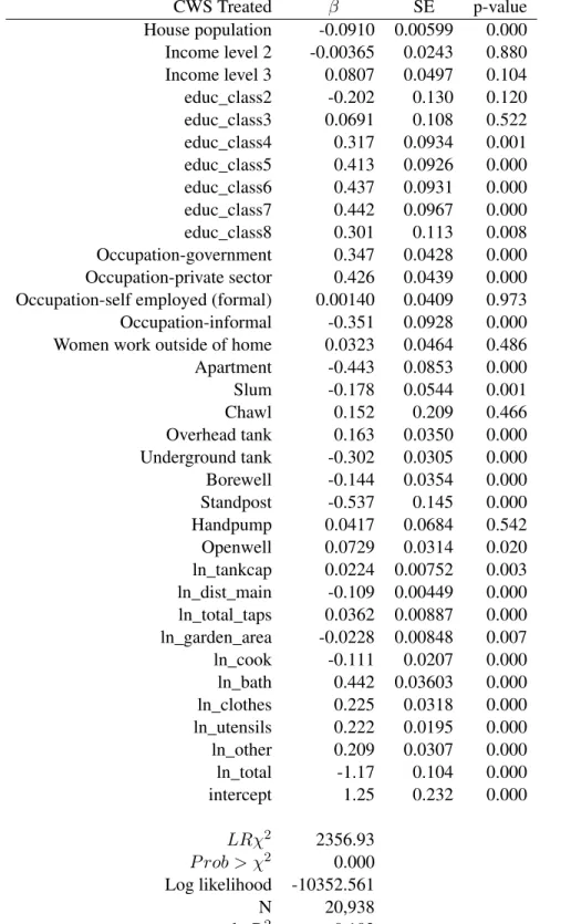
The propensity score procedure successfully alleviated some of the bias due to systematic differences between the treatment CWS households and control IWS households. Table 3 shows the probit model. Table 4 shows the mean difference between the treatment and control groups, before and after weighting by propensity score. Before weighting, there were statistically significant differences (p<0.05) between the groups in 28 out of the 35 observed time-invariant covariates. After weighting, there were only four such differences, and these differences were still reduced by the procedure. Figure 4 shows the median LPCD trend when the data weighted by propensity score. Note the higher relative demand of the IWS customers, and especially the closeness to initial demand in the Sai Nagar, HSR, and Maya Nagar CWS zones.

3.2.2 Average Treatment Effect

(38)

Table 3: Probit regression for propensity scores based on observed household characteristics

CWS Treated SE p-value

House population -0.0910 0.00599 0.000 Income level 2 -0.00365 0.0243 0.880 Income level 3 0.0807 0.0497 0.104 educ_class2 -0.202 0.130 0.120 educ_class3 0.0691 0.108 0.522 educ_class4 0.317 0.0934 0.001 educ_class5 0.413 0.0926 0.000 educ_class6 0.437 0.0931 0.000 educ_class7 0.442 0.0967 0.000

educ_class8 0.301 0.113 0.008

Occupation-government 0.347 0.0428 0.000 Occupation-private sector 0.426 0.0439 0.000 Occupation-self employed (formal) 0.00140 0.0409 0.973 Occupation-informal -0.351 0.0928 0.000 Women work outside of home 0.0323 0.0464 0.486

Apartment -0.443 0.0853 0.000

Slum -0.178 0.0544 0.001

Chawl 0.152 0.209 0.466

Overhead tank 0.163 0.0350 0.000 Underground tank -0.302 0.0305 0.000 Borewell -0.144 0.0354 0.000

Standpost -0.537 0.145 0.000

Handpump 0.0417 0.0684 0.542

Openwell 0.0729 0.0314 0.020

ln_tankcap 0.0224 0.00752 0.003 ln_dist_main -0.109 0.00449 0.000 ln_total_taps 0.0362 0.00887 0.000 ln_garden_area -0.0228 0.00848 0.007

ln_cook -0.111 0.0207 0.000

ln_bath 0.442 0.03603 0.000

ln_clothes 0.225 0.0318 0.000

ln_utensils 0.222 0.0195 0.000

ln_other 0.209 0.0307 0.000

ln_total -1.17 0.104 0.000

intercept 1.25 0.232 0.000

LR 2 _2356.93

P rob > 2 0.000

Log likelihood -10352.561

N 20,938

pseudo-R2 _0.102

(39)

Table 4: Observed covariates over continuous water supply treatment before and after Propensity Score Matching

Mean t-test Mean t-test

Variable Treated Control t p-value Variable Treated Control t p-value House population Unmatched 4.47 4.99 -15.030 0.000 Is a Chawl Unmatched 0.00 0.00 -0.230 0.816

Matched 4.47 4.53 -1.910 0.056 Matched 0.00 0.00 -0.280 0.778

Income level 2 Unmatched 0.34 0.26 10.330 0.000 Has overhead tank Unmatched 0.67 0.53 17.410 0.000 Matched 0.34 0.33 0.620 0.535 Matched 0.67 0.65 1.700 0.089

Income level 3 Unmatched 0.05 0.04 3.860 0.000 Has underground tank Unmatched 0.41 0.53 -14.730 0.000 Matched 0.05 0.05 -0.310 0.756 Matched 0.41 0.42 -0.860 0.388

educ_class2 Unmatched 0.01 0.02 -6.750 0.000 Uses private borewell Unmatched 0.09 0.09 0.610 0.544 Matched 0.01 0.01 -0.990 0.324 Matched 0.09 0.10 -0.560 0.575

educ_class3 Unmatched 0.02 0.05 -8.790 0.000 Uses public standpost Unmatched 0.00 0.01 -3.190 0.001 Matched 0.02 0.02 -0.860 0.388 Matched 0.00 0.00 -0.070 0.941

educ_class4 Unmatched 0.17 0.23 -9.450 0.000 Uses public handpump Unmatched 0.02 0.02 -0.320 0.747 Matched 0.17 0.18 -1.150 0.249 Matched 0.02 0.02 -0.110 0.910

educ_class5 Unmatched 0.29 0.29 0.290 0.768 Uses private dug well Unmatched 0.13 0.11 4.060 0.000 Matched 0.29 0.29 0.030 0.977 Matched 0.13 0.13 -0.010 0.996

educ_class6 Unmatched 0.35 0.27 10.650 0.000 ln(storage tank capacity (kL) Unmatched 5.49 5.32 4.310 0.000 Matched 0.35 0.34 0.410 0.680 Matched 5.49 5.43 1.180 0.237

educ_class7 Unmatched 0.13 0.09 6.970 0.000 ln(tap distance from water main (m)) Unmatched 0.67 1.49 -22.740 0.000 Matched 0.13 0.12 1.370 0.172 Matched 0.67 0.83 -2.850 0.004

educ_class8 Unmatched 0.03 0.02 1.760 0.079 ln(number of taps in house) Unmatched 0.59 0.49 4.950 0.000 Matched 0.03 0.02 0.440 0.660 Matched 0.59 0.54 1.720 0.085

Occupation-government Unmatched 0.40 0.28 16.580 0.000 ln(garden size sq. m) Unmatched -4.43 -4.42 -0.510 0.612 Matched 0.40 0.38 2.220 0.027 Matched -4.43 -4.41 -0.770 0.444

Ocucpation-private sector Unmatched 0.25 0.18 11.430 0.000 ln_cook Unmatched 1.25 1.32 -6.720 0.000 Matched 0.25 0.25 0.540 0.589 Matched 1.25 1.27 -1.940 0.052

Occupation-self employed (formal) Unmatched 0.28 0.42 -18.020 0.000 ln_bath Unmatched 2.88 2.81 8.610 0.000 Matched 0.28 0.30 -2.860 0.004 Matched 2.88 2.88 0.610 0.539

Occupation-informal Unmatched 0.01 0.03 -6.610 0.000 ln_clothes Unmatched 2.48 2.52 -3.280 0.001 Matched 0.01 0.01 -0.310 0.755 Matched 2.48 2.52 -2.820 0.005

Occupation-other Unmatched 0.06 0.10 -8.490 0.000 ln_utensils Unmatched 2.15 2.13 1.890 0.058 Matched 0.06 0.06 0.050 0.959 Matched 2.15 2.15 0.400 0.690

Women work outside of home Unmatched 0.05 0.05 2.740 0.006 ln_other Unmatched 2.39 2.44 -3.220 0.001 Matched 0.05 0.05 0.070 0.941 Matched 2.39 2.40 -0.110 0.913

Is an Apartment Unmatched 0.01 0.02 -3.940 0.000 ln_total Unmatched 4.10 4.13 -4.080 0.000 Matched 0.01 0.01 0.000 0.999 Matched 4.10 4.12 -1.630 0.103

Is a Slum dwelling Unmatched 0.03 0.06 -8.300 0.000 Matched 0.03 0.03 -1.150 0.249

(40)

60# 70# 80# 90# 100# 110# 120# 130# 140# 150# 160# 170# 180# N OV /09# J AN /10# M AR /10# M AY /10# J UL /10# S EP /10# N OV /10# J AN /11# M AR /11# M AY /11# J UL /11# S EP /11# N OV /11# J AN /12# M AR /12# M AY /12# J UL /12# S EP /12# N OV /12# J AN /13# Me di an 'B im on th ly 'Me te re d' W at er 'C on su m p5 on '(L PC D )' _IWS# Arjun#Nagar# Sai#Nagar# HSR# Maya#Nagar#

Figure 4: Median lpcd in Amravati domestic water connections, October-November 2009 to December-January 2013 (weighted)

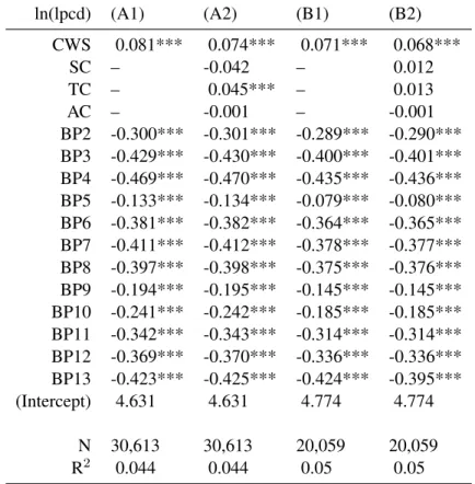
regressors. The basic model (A1) estimates an average treatment effect of CWS of an additional 8.1% of water consumption per person in the household. This effect is still present in the propensity-score matched model (B1), although the estimate is reduced to 7.1%. In the model (A2) including interaction terms for being in a slum (SC), having an external storage tank (TC), and having an alternate water source (AC), there is a significant positive coefficient of 0.045 for TC. However, this coefficient is not significant in the model (B2) with propensity score weighting. Taken together, these results indicate that there was, on average, a statistically significant positive effect on consumption from CWS in Amravati over the first 3 years. Any differences, on average, in the effect between slum dwellers and non slum dwellers, households with and without tanks, and households with and without alternate water supplies, were not found to be significant.

3.2.3 Distributional Impacts

(41)

Table 5: The average effect of continuous water supply on water demand

ln(lpcd) (A1) (A2) (B1) (B2)

CWS 0.081*** 0.074*** 0.071*** 0.068***

SC – -0.042 – 0.012

TC – 0.045*** – 0.013

AC – -0.001 – -0.001

BP2 -0.300*** -0.301*** -0.289*** -0.290*** BP3 -0.429*** -0.430*** -0.400*** -0.401*** BP4 -0.469*** -0.470*** -0.435*** -0.436*** BP5 -0.133*** -0.134*** -0.079*** -0.080*** BP6 -0.381*** -0.382*** -0.364*** -0.365*** BP7 -0.411*** -0.412*** -0.378*** -0.377*** BP8 -0.397*** -0.398*** -0.375*** -0.376*** BP9 -0.194*** -0.195*** -0.145*** -0.145*** BP10 -0.241*** -0.242*** -0.185*** -0.185*** BP11 -0.342*** -0.343*** -0.314*** -0.314*** BP12 -0.369*** -0.370*** -0.336*** -0.336*** BP13 -0.423*** -0.425*** -0.424*** -0.395***

(Intercept) 4.631 4.631 4.774 4.774

N 30,613 30,613 20,059 20,059

R2 _0.044 _0.044 _0.05 _0.05

Notes:Dependent variable: Natural log of bimonthly household water consumption (lpcd). Model (A1) includes only the CWS treatment with billing period and household fixed effects. Model (A2) includes interactions between CWS and slum (SC) having an external storage tank (TC) and having an alternate water source (AC). Model (B1) is the same as (A1), with panels weighted by propensity score. Model (B2) is the same as (B1), with panels weighted by propensity score.

Significance:*p<.05, **p<.01, ***p<.001

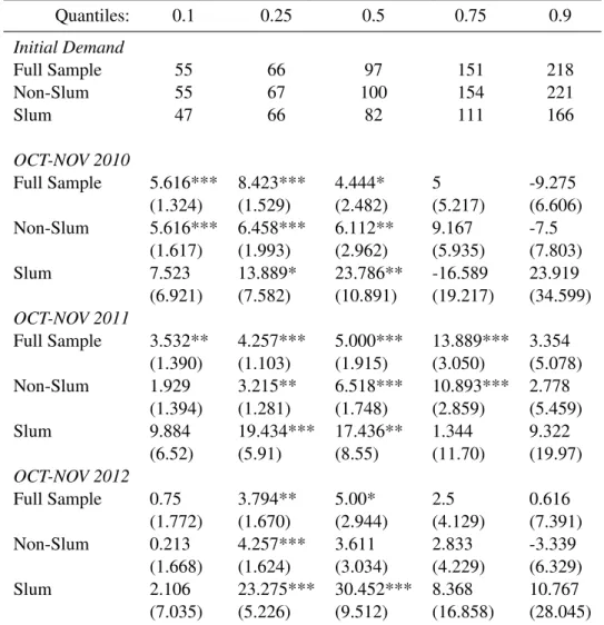
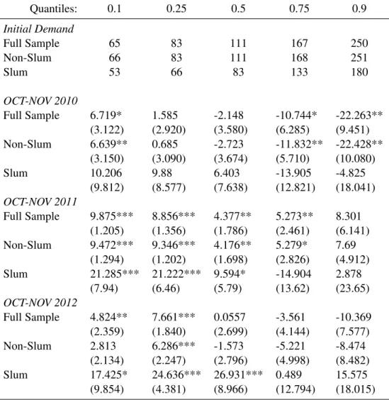
For the model where the second period is October-November 2010, without weighting, the model shows modest increases of about 5-6 lpcd due to CWS among non-slum households that were consuming below the median in the initial period. Slum households show no significant effects except for at the median, where a substantial increase of 24 lpcd is estimated. However, with propensity score weighting, in this period there is no detected effect in slum households, while non-slum households show significant decreases of 11-22 lpcd in the upper quantiles.

(42)

Table 6: Quantile difference-in-differences, effects of continuous water supply on lpcd

Quantiles: 0.1 0.25 0.5 0.75 0.9

Initial Demand

Full Sample 55 66 97 151 218

Non-Slum 55 67 100 154 221

Slum 47 66 82 111 166

OCT-NOV 2010

Full Sample 5.616*** 8.423*** 4.444* 5 -9.275

(1.324) (1.529) (2.482) (5.217) (6.606)

Non-Slum 5.616*** 6.458*** 6.112** 9.167 -7.5

(1.617) (1.993) (2.962) (5.935) (7.803)

Slum 7.523 13.889* 23.786** -16.589 23.919

(6.921) (7.582) (10.891) (19.217) (34.599)

OCT-NOV 2011

Full Sample 3.532** 4.257*** 5.000*** 13.889*** 3.354 (1.390) (1.103) (1.915) (3.050) (5.078)

Non-Slum 1.929 3.215** 6.518*** 10.893*** 2.778

(1.394) (1.281) (1.748) (2.859) (5.459)

Slum 9.884 19.434*** 17.436** 1.344 9.322

(6.52) (5.91) (8.55) (11.70) (19.97)

OCT-NOV 2012

Full Sample 0.75 3.794** 5.00* 2.5 0.616

(1.772) (1.670) (2.944) (4.129) (7.391)

Non-Slum 0.213 4.257*** 3.611 2.833 -3.339

(1.668) (1.624) (3.034) (4.229) (6.329)

Slum 2.106 23.275*** 30.452*** 8.368 10.767

(7.035) (5.226) (9.512) (16.858) (28.045)

Notes:Top rows show initial demand for each sample at each quantile of initial water demand. Dependent variable: Bimonthly household water consumption (lpcd). Bootstrapped standard errors of the mean effect in parentheses.

(43)

Table 7: Quantile difference-in-differences with kernel propensity score weighting, effects of continuous water supply on lpcd

Quantiles: 0.1 0.25 0.5 0.75 0.9

Initial Demand

Full Sample 65 83 111 167 250

Non-Slum 66 83 111 168 251

Slum 53 66 83 133 180

OCT-NOV 2010

Full Sample 6.719* 1.585 -2.148 -10.744* -22.263**

(3.122) (2.920) (3.580) (6.285) (9.451)

Non-Slum 6.639** 0.685 -2.723 -11.832** -22.428**

(3.150) (3.090) (3.674) (5.710) (10.080)

Slum 10.206 9.88 6.403 -13.905 -4.825

(9.812) (8.577) (7.638) (12.821) (18.041)

OCT-NOV 2011

Full Sample 9.875*** 8.856*** 4.377** 5.273** 8.301 (1.205) (1.356) (1.786) (2.461) (6.141)

Non-Slum 9.472*** 9.346*** 4.176** 5.279* 7.69

(1.294) (1.202) (1.698) (2.826) (4.912)

Slum 21.285*** 21.222*** 9.594* -14.904 2.878

(7.94) (6.46) (5.79) (13.62) (23.65)

OCT-NOV 2012

Full Sample 4.824** 7.661*** 0.0557 -3.561 -10.369

(2.359) (1.840) (2.699) (4.144) (7.577)

Non-Slum 2.813 6.286*** -1.573 -5.221 -8.474

(2.134) (2.247) (2.796) (4.998) (8.482)

Slum 17.425* 24.636*** 26.931*** 0.489 15.575

(9.854) (4.381) (8.966) (12.794) (18.015)

Notes:Top rows show initial demand for each sample at each quantile of initial water demand. Dependent variable: Bimonthly household water consumption (lpcd). Bootstrapped standard errors of the mean effect in parentheses.

(44)

poorest (connected) households who were consuming low amounts of water to begin with, but not much of an effect for slum households consuming more water.

For the models where the second period is October-November 2012, the effects are similar but more modest, and restricted to the 0.5 quantile and below for non-slum households. This may reflect long-run adjustments. However, the second price increase in July 2012 may also be a contributing factor. This price increase raised the price of water in the lowest block as well as the upper blocks, so it is possible that the effects are more modest at the lower quantiles than before due to a reaction to this price. Reductions in consumption in the upper quantiles return in this period, although they are not significant. The effect in slum households is not moderated in this period, however.

3.3 Component 2: Coping Behaviors

3.3.1 Summary of primary survey

Table 12 and Table 13 in Appendix D summarize responses to direct questions about coping behaviors. In this section, tabulated results are supplemented with illustrative examples from households that volunteered elaborations. 48 households were interviewed in Nagpur (22 in CWS and 26 in IWS zones) and 46 households in Amravati (21 in CWS and 25 in IWS zones). The targeted sample sizes were not attained primarily due to time constraints. For example, only 10 total slum households out of a target of 20 were interviewed in Amravati because connected slum households were so rare that not enough examples could be found that would consent to be interviewed. The target sample sizes were exceeded for non-slum households with IWS in Nagpur and with IWS and CWS in Amravati because members of neighboring households became curious and requested to be interviewed.

3.3.2 Storage

Storage behavior responses in Nagpur and Amravati under IWS and CWS conditions are summarized for non-slum and slum households in Figure 5 and Figure 6, respectively.

Storage under intermittent water supply

(45)

0%# 10%# 20%# 30%# 40%# 50%# 60%# 70%# 80%# 90%# 100%#

IWS#(n=16)# CWS#(n=14)# IWS#(n=20)# CWS#(n=16)#

Nagpur# Amrava>#

Percen

ta

ge)o

f)h

ou

seh

ol

ds)i

n)ea

ch

)CWS

/I

WS

7ci

ty

)co

mb

in

a;o

n)rep

or;n

g)b

eh

avi

or)

Overhead#Tank# Sump#

Drums#

Kitchen#Storage#in#Pots#

Figure 5: Percentage of non-slum households exhibiting storage behaviors

(46)

0%# 10%# 20%# 30%# 40%# 50%# 60%# 70%# 80%# 90%# 100%#

IWS#(n=10)# CWS#(n=8)# IWS#(n=5)# CWS#(n=5)#

Nagpur# Amrava>#

Percen

ta

ge)h

ou

seh

ol

ds)i

n)ea

ch

)CWS

/I

WS

6Ci

ty

)co

mb

in

a:o

n)rep

or:n

g)b

eh

avi

or)

Overhead#Tank# Sump#

Drums#

Kitchen#Storage#in#Pots#

Figure 6: Percentage of slum households exhibiting storage behaviors

KyleOnda_MSPHFinal.pdf

ABSTRACT

ACKNOWLEDGEMENTS

TABLE OF CONTENTS

LIST OF TABLES

LIST OF FIGURES

LIST OF ABBREVIATIONS

1 Introduction

2 Methods

3 Results