COMPARING LOW-REDSHIFT COMPACT DWARF STARBURSTS IN THE RESOLVE SURVEY WITH HIGH-REDSHIFT BLUE NUGGETS
Michael L. Palumbo III,1 Sheila J. Kannappan,1 Elaine M. Snyder,2 Kathleen D. Eckert,3Dara Norman,4
Luciano Fraga,5 Bruno Quint,6Philippe Amram,7 Claudia Mendes de Oliveira,8 Ashley Bittner,9 Amanda Moffett,10 David Stark,11 Mark Norris,1 and Nate T. Cleaves1
1University of North Carolina at Chapel Hill 2Space Telescope Science Institute
3University of Pennsylvania
4National Optical Astronomy Observatory
5Laborat´orio Nacional de Astrof´ısica Coordenadoria de Apoio a Ciencia 6Southern Astrophysical Research Telescope (SOAR)
7Laboratoire d’Astrophysique de Marseille 8Universidade de S˜ao Paulo
9North Carolina State University 10Vanderbilt University
11Kavli Institute for the Physics and Mathematics of the Universe
(Revised April 26, 2018)
ABSTRACT
We identify and characterize compact dwarf starburst galaxies in the RESOLVE survey, a volume-limited census of galaxies in the local universe, to probe the extent to which these galaxies are analogous to “blue nuggets,” a class of intensely star-forming compact dwarf galaxies at high redshifts. We compare the masses, star formation rates, stellar surface mass densities, projected axis ratios, and environmental contexts of our sample to expectations and observations of blue nuggets. We find that low-z blue nugget candidates in the RESOLVE survey are statistically analogous to their high-z counterparts, exhibiting masses, colors, and specific star formation rates (SSFR) consistent with past high-z observations. However, we find that the stellar surface mass densities of our low-z sample are on order 108 M kpc 2, or about a dex lower than what is predicted and observed for high-z blue nuggets. Cosmological simulations and semianalytical models in recent years have suggested that blue nuggets form as the result of intense compaction events driven by either converging cosmic gas streams or wet minor mergers. In either formation scenario, simulations have additionally suggested that these galaxies should exhibit some degree of rotation along their minor axes and prolate morphology. We report 3D spectroscopy observations of four of low-z blue nugget analogues, from which we construct high-resolution velocity fields, examining the evidence for minor axis or otherwise misaligned rotation. We observe evidence for double nuclei in ⇠85% of our low-z blue nugget analogue sample, strongly favoring a merger origin for these objects. We additionally observe dynamically complex kinematics in the 3D spectroscopy observations with multiple components of rotation which are spatially consistent with the double nuclei detections, further suggesting recent wet minor mergers as the dominant formation mechanism for our low-z blue nugget analogues.
1. INTRODUCTION
The first observations of a class of compact massive (Mstar & 1011M ) elliptical galaxies with suppressed
star formation rates at z ⇠ 2 3 (van Dokkum et al. 2008; Ilbert et al. 2010) posed an evolutionary mys-tery. These galaxies, known technically as red quies-cent galaxies (Barro et al. 2013) or colloquially as “red nuggets” (Damjanov et al. 2009; Newman et al. 2010), are extraordinarily compact with radii up to⇠5 times smaller than typical galaxies of comparable mass in the low-z universe (Trujillo et al. 2007; Toft et al. 2007;
Williams et al. 2014). The extreme stellar density of these objects has completely ruled out simple mono-lithic models of formation (as described inEggen et al. 1962), which exclude significant structural evolution fol-lowing initial galaxy assembly at very high redshifts (van Dokkum et al. 2008). Moreover, major merger mod-els cannot account for the observed compactness of red nuggets, since these non-dissipative events preferentially scatter pre-existing stars to larger orbital radii, “puffing up” rather than compacting the resulting object (Naab et al. 2007;Naab & Ostriker 2009).
More recently, cosmological simulations (such as in
Ceverino et al. 2015; Tacchella et al. 2016) have sug-gested that minor, wet mergers favorably produce rem-nants with ultra-compact cores as a result of the dissipa-tive nature of the gas allowing for angular momentum loss (Khochfar & Silk 2006; Hopkins et al. 2008). In-deed, complementary observations have pinned a class of compact star-forming dwarf galaxies known as “blue nuggets” as suitable evolutionary progenitors for red nuggets (Patel et al. 2013;Barro et al. 2013;Nelson et al. 2014). Using a toy model,Dekel & Burkert (2014) an-alytically demonstrate that inflow from smooth cosmic streams and minor wet mergers generate sufficient an-gular momentum loss to account for the extraordinary compactness of red nuggets. They show the extreme gas inflow ignites a chain of events, culminating in violent disk instability, contraction, and rapid star formation so long as the rate of dissipative gas inflow exceeds the rate of star formation in the central regions of the galaxy, creating a blue nugget. Without a fresh supply of gas, these blue nuggets eventually quench, evolving into the observed red nugget phase.
Analyses of the observed projected ellipticities of galaxies at z > 1 have shown that the distribution of galaxy morphologies at at high redshift are predomi-nately triaxial (Law et al. 2012). Follow up analyses by
Chang et al. (2013) and van der Wel et al.(2014) have together demonstrated that the oblate fraction of galax-ies with Mstar <1010.5M increases with cosmic time,
and that most galaxies with Mstar ⇠108.5 109.5M
at z ⇠1 2 are prolate, suggesting that the evolution from the blue nugget phase to the red nugget phase, as outlined by Dekel & Burkert (2014), should also include an evolution in morphology. Indeed, cosmolog-ical simulations of blue nuggets have shown that the minor merger formation scenario should create prolate objects (Jing & Suto 2002; Bailin & Steinmetz 2005;
Allgood et al. 2006), whose major axes are preferen-tially aligned with the larger filamentary structure of the cosmic web in which they are embedded (Codis et al. 2015; Laigle et al. 2015). Additional simulations per-formed by Tomassetti et al.(2016) have shown torques induced by the dark matter (DM) halo during the gas compaction event are capable of elongating the stellar system into a prolate shape. Simulations conducted by
Tomassetti et al.(2016) andCeverino et al.(2015) both reveal that blue nuggets tend to display some degree of characteristic rotation along their minor axes.
Tacchella et al.(2016) show that blue nuggets undergo successive cycles of compaction and quenching, so long as there is a fresh supply of gas to replenish central star formation. They predict that this “self-regulated evo-lution” ultimately tends toward a red nugget when hot halo quenching dominates at virial massMvir ⇠1011.5,
corresponding to a stellar mass on order Mstar ⇠1010
at most. Dekel & Burkert(2014) surmise that the self-regulated evolution of blue nuggets is dependent upon “fast-mode” growth, which allows for extremely rapid star formation, mass accretion, and ultimately rapid quenching driven by hot halos. In the opposite case of “slow-mode” growth, slower gas accretion regulates the rapid formation of stars, slowing progress across the red sequence. The rapid appearance of a red sequence on the scale of ⇠ 0.7 Gyr, as shown by Barro et al.
(2013), is consistent with the relatively rapid quenching characteristic of fast-mode accretion.
it is currently unclear whether the fast-mode accretion, which is dependent upon very high gas fractions and therefore preferential to the high redshifts, can occur in the present day universe. Indeed, Dekel & Burkert
(2014) calculate that the fraction of galaxies which be-come blue nuggets depends primarily upon the fraction of cold gas mass with respect to baryon mass, a pa-rameter which decreases dramatically with cosmic time. Observations by van der Wel et al. (2014) correspond-ingly show that the fraction of prolate galaxies with Mstar .109.5, namely blue nuggets, decreases
dramat-ically from z = 2 to z = 0. However, this fraction is non-vanishing atz= 0 despite its strong dependence on cosmic time. The non-zero prolate galaxy fraction com-bined with the observation of massive compact quiescent galaxies (i.e. red nuggets) at intermediate redshifts as low as z ⇠0.1 by Damjanov et al. (2015) suggests the possibility of fast-mode accretion and quenching occur-ring in the intermediate- and low-z universe.
We therefore desire to examine the existence and na-ture of blue nuggets in the low-z universe. Is there a population of compact starburst dwarfs in the present-day universe analogous to high-z blue nuggets? Do they exhibit prolate morphology and rotation along their mi-nor axes? Do they form by the same two mechanisms proposed at high-z (i.e. wet minor mergers and colliding cosmic streams)?
To answer these questions, we turn to the REsolved Spectroscopy Of a Local VolumE (RESOLVE) Survey1,
a volume-limited census of galaxies in the local universe, whose statistical completeness and low mass floor is ideal for identifying and characterizing a population of galax-ies nearly a full dex lower in mass than theBarro et al.
(2013) blue nugget sample. We present the identifica-tion of a populaidentifica-tion of 35 low-z blue nugget candidates in RESOLVE. We examine the key statistical features of the low-z candidate sample, comparing to high-z blue nuggets in order to characterize the exact relationship between the present-day and distant-past populations. By studying the star formation rates and morphologies of the low-z blue nugget candidates, we probe the evolu-tionary relationship of these objects to their high-z coun-terparts. By studying the distributions of nearest neigh-bor distances and rate of double nucleus occurrence, we examine the possible formation mechanisms of the low-z blue nugget candidates, and therefore the nature of fast-mode accretion in the present-day universe.
In order to further address the formation history of the low-z blue nugget candidate population, we use
follow-1https://resolve.astro.unc.edu/
up 3D spectroscopy to probe the internal structure and kinematics of four candidate galaxies. We compare the structure of these individual galaxies to expectations from high-z simulations by:
i. constructing and modeling velocity fields to search for minor-axis, misaligned, or multi-component ro-tation as revealed in simulations by Ceverino et al.
(2015) andTomassetti et al.(2016)
ii. creating continuum and H↵flux maps to search for or confirm double nuclei as a probe of the wet minor merger mechanism of fast-mode growth
This work is laid out as follows. In section 2 we de-scribe the RESOLVE survey, our sample selection, and the follow-up 3D spectroscopy data. Insection 3we dis-cuss our analysis of the 3D spectroscopy data, including velocity fields, continuum maps, and H↵line flux maps. Insection 4we examine the formation and environments of the low-z blue nugget candidate sample, in addition to making statistical comparisons to the literature high-z blue nugget populations. Insection 5 discuss the rela-tionship between the low-z and high-z population, ex-amining whether the present-day candidates are actu-ally blue nuggets or simply analogous, but not identical, entities. Finally, insection 6we summarize our findings. We assume a standard⇤CDM cosmology with⌦m=
0.3,⌦⇤= 0.7, andH0= 70 km s 1 Mpc 1 for distance measurements and other derived quantities in this work.
2. DATA
2.1. The RESOLVE Survey
For this work, we use the RESOLVE (REsolved Spec-troscopy of a Local VolumE) survey, a volume-limited census of galaxies in the local universe with the goal of accounting for baronyic and dark matter mass within a statistically complete subset of the z ⇠ 0 galaxy pop-ulation. As a result of the volume-limited nature, RE-SOLVE is ideal for examining the properties of the full low-z blue nugget candidate population without the sta-tistical completeness corrections endemic to flux-limited surveys. Moreover, the low mass floor of RESOLVE al-low us to probe deeper into the prolate mass regime of Mstar <109.5 observed byvan der Wel et al.(2014), as
opposed to theMstar >1010 mass limit of Barro et al.
(2013) which lies above the prolate mass regime.
2.1.1. Survey Definition and Ancillary Data
-100 -50 0 50 100 Mpc
-100 -50 0 50 100
Mpc
RESOLVE-A
RESOLVE-B
Figure 1. RESOLVE survey footprint with low-z blue
nugget candidates (seesection 2.1.2) highlighted as red stars.
bounded in Local Group-corrected heliocentric velocity from VLG = 4500 7000 km s 1. To avoid situations
where peculiar velocities may a↵ect survey membership, group (rather than individual) redshifts are used to de-cide final survey membership. RESOLVE is contained within the SDSS footprint and uses the SDSS redshift survey to build survey membership. In addition to redshifts measurements obtained from RESOLVE ob-servations (Kannappan et al. 2018, in prep.), we include additional redshifts from a number of archival sources: the Update Zwicky Catalog (Falco et al. 1999), Hyper-Leda (Paturel et al. 2003), 6dF (Jones et al. 2009), 2dF (Colless et al. 2001), GAMA (Driver et al. 2011), and ALFALFA (Haynes et al. 2011).
As shown in Kannappan et al. (2013) and Eckert et al.(2016), RESOLVE-A is complete down toMr,tot=
17.33, which roughly corresponds to a baryonic mass completeness limit of log(Mbary/M ) = 9.3. For the
slightly deeper RESOLVE-B, the luminosity complete-ness limit of Mr,tot = 17.0 corresponds to a baryonic
mass completeness limit of log(Mbary/M ) = 9.1 and a
stellar mass completeness limit of log(Mstar/M ) = 8.7.
As described in Eckert et al. (2015) RESOLVE employs reprocessed photometric data from the UV through NIR. RESOLVE data in the opticalugrizcomes from SDSS (Aihara et al. 2011), NIRJHK from 2MASS (Skrutskie et al. 2006) and/or YHK from UKIDSS (Hambly et al. 2008), and NUV from GALEX ( Mor-rissey et al. 2007). The reprocessed RESOLVE pho-tometry improves on SDSS pipeline phopho-tometry as the result of improved sky subtraction, improved elliptical apertures generated from summed high signal-to-noise
ratio (SNR) gri images, and the use of non-parametric models of magnitude extrapolation (among other factors discussed in detail inEckert et al. 2015). RESOLVE stel-lar masses are calculated from the SED modeling code described inKannappan & Gawiser(2007) and Kannap-pan et al.(2013), which uses photometric data from up to 10 bands to provide robust estimates of stellar mass. The HI masses and upper limits are obtained from deep, pointed observations with the GBT and Arecibo telescopes supplementing the blind 21 cm ALFALFA survey (Haynes et al. 2011), and are calculated as in
Kannappan et al.(2013) andStark et al.(2016). Group finding is performed using the Friends-of-Friends algo-rithm as described in (Berlind et al. 2006) and justified in (Eckert et al. 2016). Group halo masses are assigned by using halo abundance matching between identified groups and the theoretical halo mass function ofWarren et al. (2006), as described inBerlind et al. (2006) and
Mo↵ett et al. (2015). RESOLVE de-extincted central H↵fluxes are obtained by Balmer decrement measure-ments and foreground extinction corrections of SDSS central flux measurements using the Milky Way ex-tinction curve of O’Donnell (1994) as given by McCall
(2004).
2.1.2. Sample Definition
We identify a sample of 35 blue nugget candidate galaxies in the RESOLVE Survey. Guided by the ob-served and simulated properties of high-z blue nuggets in literature, we have constrained our candidate blue nuggets to a region of parameter space containing highly compact, possibly prolate galaxies in the dwarf mass regime. We implement selectors in stellar mass, mor-phology, color, and specific star formation rate (SSFR):
• Theoretical study (Ceverino et al. 2015) and obser-vations (van der Wel et al. 2014) of prolate galax-ies has shown that hot halo quenching begins to shut down cosmic gas accretion in blue nuggets above stellar mass log(Mstar/M )⇠9.5. We
lect objects below this mass threshold. Our se-lection also includes an explicit mass floor, cor-responding to the completeness limit of the RE-SOLVE survey: log(Mbary/M ) = 9.3 M and
log(Mbary/M ) = 9.1 respectively for
RESOLVE-A and -B, where Mbary is the combined mass of
cold gas and stars.
quantita-(a) (b)
(c)
Figure 2. Selection plots for low-z blue nuggets. (a) For their mass, blue nugget candidates are among the most compact
objects in the RESOLVE survey, reflecting the intense compaction events that have driven their starbursts. (b) The selection of log(SSFR [Gyr 1])> 0.5, as in theBarro et al.(2013) sample, isolates some of the most intense starbursts in RESOLVE. Note that the y-axis is inverted for the sake of consistency with theBarro et al.(2013) standard. (c) Blue nugget candidates sit well within the blue sequence of RESOLVE.
tive surrogate for Hubble type2. Restricting our
sample to µ > 8.6 limits our sample to bulged disk and spheroid-dominated galaxies with high degrees of concentration of central star formation (Figure 2a).
• Dekel & Burkert (2014) show that blue nuggets should be found on the blue end of the blue se-quence. To select galaxies in the blue sequence of RESOLVE, we implement a color restriction of u r <1.5.
2 µ combines the overall stellar surface mass density with a stellar surface mass density contrast term:µ =µ90+1.7 µ. The
contrast term µis expressed as the di↵erence between the stellar
surface mass densities within the 50% light radius and between the 50% and 90% light radii. SeeKannappan et al.(2013).
• Blue nuggets are impressive starbursts as a re-sult of the intense gas compaction in their centers. To select galaxies undergoing starbursts similar to those at high redshift, we impose a specific star for-mation rate limit of log(SSFR [Gyr 1])> 0.5 as in Barro et al. (2013). Accordingly, we find that this restriction simultaneously selects RESOLVE galaxies whose de-extincted central H↵ fluxes lie in the upper⇠50th percentile (Figure 3, right).
2.2. 3D Spectroscopic Data
Hα
Hβ OIII
OIII
NII NII H!
Figure 3. Left: SIFS spectrum for rs1103 displaying dominant H↵ and [OIII] emission lines typical of blue
nugget spectra. Powerful [OIII] emission lines are strongly indicative of metal-poor gas. The strong H↵ emission signifies
intense star formation, which is corroborated by the strong blue color in the photometry. Right: Distributions of
de-extincted H↵fluxes for RESOLVE and for compact blue dwarf galaxies.Our selection on log(SSFR [Gyr 1])> 0.5
implicitly selects RESOLVE galaxies with de-extinced central H↵fluxes in the upper 50th percentile.
sample galaxy spectra at each lenslet position. Com-pared to traditional longslit spectroscopy, integral field spectroscopy allows us to easily construct spatially-resolved velocity fields of extended objects by sampling object spectra at ⇠1000 discrete points (in the case of the GMOS IFU) and arranging these spectra into “pseu-doslits” whose light is dispersed onto the detector. In a di↵erent vein, SAM FP uses an etalon to image a target at discrete wavelengths within a narrow spectral range. In comparison to IFU instruments, the SAM FP is able to sample at a much higher spatial frequency at the ex-pense of spectral range.
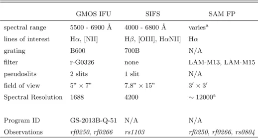
To extract spatially-resolved velocity and continuum information, we rely primarily upon the strong H↵ emis-sion line. Depending on the wavelength range of the instrument setup, we may also use the [NII] doublet, the [OIII] doublet, and H . In all cases, the field-of-view must cover the full spatial extent of emission for the galaxy. In several cases, this has necessitated spa-tial tiling of exposures. The centroiding accuracy of the H↵ line should be ⇠5 km/s at the half-light radius of galaxy to avoid unacceptable errors in velocity calcula-tions. Table 1 contains a summary of the instrument setups.
In order to probe the dynamical properties of our ob-jects, we require reduced data cubes with spatial infor-mation in the x-y plane, and spectral inforinfor-mation along the z-axis. From these we obtain spatially resolved ve-locity fields, continuum maps, and H↵ flux maps, as described in section 3.1. These plots serve as our pri-mary evidence for i) minor-axis or misaligned rotation and ii) double nuclei detection.
For the GMOS IFU data we have developed the Gem-ini Reduction Pipeline in order to efficiently and accu-rately transform the two-dimensional observational data into three-dimensional data cubes. For a description of the Gemini reduction process, seeAppendix A. Since we obtained the SIFS and SAM FP data in science verifica-tion (SV) time, the respective SV teams performed the data reduction into data cubes. The SAM FP reduction was performed as described inMendes de Oliveira et al.
(2017), including calibrations analogous to the GMOS IFU reduction (e.g. bias subtraction, wavelength cali-bration, cosmic ray rejection, etc.). We additionally perform astrometrical calibration on the SAM FP data by matching field stars in the Aladin Sky Atlas desk-top program (Bonnarel et al. 2000). The SIFS data reduction is performed in a process largely analogous to the GMOS IFU reduction process (including bias sub-traction, flat fielding, cosmic ray removal, etc.). How-ever, an additional side-step calibration is required to extract the fiber spectra due to the dense packing of in-formation along the spatial direction on the CCD, which would otherwise lead to severe fiber “cross-talk” in the extracted spectra (private communication with Luciano Fraga, Fraga et al. in prep).
2.3. DECaLS
We supplement our analysis of low-z blue nugget can-didate formation scenarios via double nucleus detection (section 4.2.1) with photometry from Data Release 5 (DR5) of the Dark Energy Camera Legacy Survey (DE-CaLS)3.
Table 1. Summary of spectroscopic instrument setups.
GMOS IFU SIFS SAM FP
spectral range 5500 - 6900 ˚A 4000 - 6800 ˚A variesa
lines of interest H↵, [NII] H , [OIII], H↵NII] H↵
grating B600 700B N/A
filter r-G0326 none LAM-M13, LAM-M15
pseudoslits 2 slits 1 slit N/A
field of view 5”⇥7” 7.8”⇥15” 30⇥30
Spectral Resolution 1688 4200 ⇠12000a
Program ID GS-2013B-Q-51 N/A N/A
Observations rf0250,rf0266 rs1103 rf0250,rf0266,rs0804
aThe wavelength range and spectral resolution of SAM FP are dependent on the free
spectral range (FSR). The central wavelength of the FSR is chosen to correspond to the mean heliocentric velocity of the observed object. SeeMendes de Oliveira et al.
(2017).
DECaLS images are initially calibrated using the DE-Cam Community Pipeline4 before being processed by
The Tractor (Lang et al. 2016), which creates probabilis-tically motivated models and the residual images used in
section 4.2.1. The Tractor approximates galaxy profiles with mixture-of-Gaussian models (Hogg & Lang 2013) which are fit via 2 minimization using the sparse least squares solver from the SciPy package.
3. METHODS
3.1. Analyzing Spectroscopic Data Cubes The ultimate product of the 3D spectroscopy reduc-tion process is a data cube that contains spatial data on the xy-plane and spectral data on the z-axis. Since the data cubes, regardless of instrument, are in principle the same, we apply the same analysis methods to data cubes from all three instruments. We extract three key pieces of information from these data cubes: velocity fields, continuum maps, and H↵line flux maps.
We use thempfit algorithm (Markwardt 2009), trans-lated into Python by Mark Rivers, to perform a non-linear least-squares fit of the spectra with a Gaussian line model. For SAM FP, we fit a single Gaussian to the H↵line. For GMOS IFU, we fit three Gaussian curves to the [NII] and H↵ lines. For SIFS, we fit the [OIII] doublet, H , the [NII] doublet, and H↵. For a given
4 https://www.noao.edu/noao/staff/fvaldes/CPDocPrelim/ PL201_3.html
instrument, the total model spectrum is represented as the sum of individual line models and the continuum level. For a generic single line with non-zero continuum level, our model takes the form:
I
obs=
Irestpeak
p
2⇡ 2(1+z)
exp
✓
( obs
(1+z) rest) 2
2 2
rest
◆
+
I
cont (1)whereIobsis the observed intensity a function of
wave-length, Irestpeak is the peak rest frame intensity of a
given line, restis the rest frame Gaussian sigma of the
line, Icont is amplitude of the continuum, and z is the
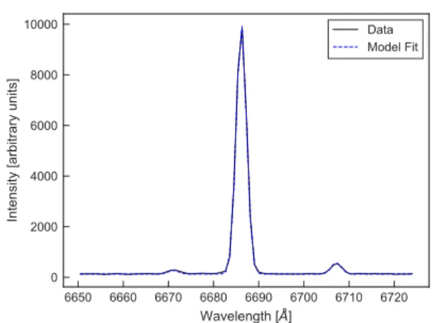
net redshift (including cosmological, peculiar, and rota-tional redshifts, as inEquation 2). This fit is performed for every spectrum in the cube, and the fitted model pa-rameters are recorded. Figure 4shows an example of a fit spectrum.
3.1.1. Velocity Fields
To produce velocity fields, we assume that the net redshift z is the product of internal rotation, peculiar motion, and cosmological redshift components:
1 +z=⇣1 +vrot c
⌘ ⇣
1 +vpec c
⌘ ⇣
1 +vcosm c
⌘
(2)
However, since we cannot disentangle peculiar and cosmological redshifts, we further assume that the pecu-liar and cosmological terms can be consolidated as such:
1 +z=⇣1 + vrot c
⌘ ⇣
1 + vhel c
⌘
Figure 4. Example spectrum extracted from GMOS
IFU data for rf0250 with Gaussian fit. The H↵
emis-sion line is plotted in blue, with the best-fit triple-Gaussian model overplotted in red. We obtain higher centroiding, and therefore velocity, accuracy by fitting to the [NII] and H↵ lines, as opposed to just H↵.
where vhel is the recessional velocity of the galaxy
in the heliocentric reference frame, estimates of which are obtained from redshift measurements as described in section 2.1.1. Rearranging Equation 3, we calculate the internal rotation velocity as:
vrot=c ✓
(1 +z)⇣1 + vhel c
⌘ 1 1
◆
, (4)
wherezis obtained from the model fit inEquation 1. We iteratively improve our measurement ofvrotby
re-measuringvhel as the average velocity in the high SNR
region of the initial velocity map. In the future, we may further improve our estimation ofvhelby employing
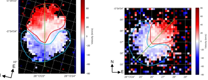
the probable minimum/maximum technique described in Kannappan et al. (2002). We find that this method produces compatible results for observations from sepa-rate instruments, as shown inFigure 5.
As shown in Tomassetti et al. (2016) and Ceverino et al. (2015), blue nuggets tend to display compli-cated rotation patterns, which are preferentially ori-ented along the minor axis. Indeed, we often ob-serve multi-component misaligned, although not purely minor-axis, rotational patterns in our velocity fields (see
section 4.1.2). We have confirmed that these complex velocity features are real physical features as opposed to erroneous detections by careful investigation of the flat-fielding (seesection A.6.1) and by comparison between observations by di↵erent instruments (seeFigure 5).
To quantify the exact magnitude and angle of the mis-alignment observed in our velocity fields, we interpret the complex velocity fields as consisting of two velocity “dipoles.” To identify the outer dipole corresponding to the bulk rotational motion of the galaxy, we first smooth
our velocity fields with a 2D median filter with kernel size 5 pixels in order to remove any spurious line fits or high frequency noise in the data. Identifying the bulk rotation is then simply a matter of finding the two po-sitions in the galaxy with the largest velocities. From these, we derive an angle and a maximum velocity for the outer rotation component. In order to quantify un-certainty on this metric, we perform 2D bootstrapping method allowing the exact values of the velocity in each spaxel to vary randomly within a Gaussian with equal to its centroiding error. We find that the error in the velocity peak positions is generally on order⇠1 arcsec-onds. The error on the min/max velocity di↵erence is typically on order⇠5 km/s.
3.1.2. Continuum and Line Flux Maps
We find continuum maps readily reveal any double nuclei, if present. The continuum level of the galaxy is simply proportional to the vertical o↵set Icont in our
Gaussian model (Equation 1).
The rapid star formation rates and low metallicities of the blue nugget candidates means that the H↵ and [OIII] lines are significant sources of flux. As a result H↵ flux maps are a promising probe of structure compared to the lower level continuum light. For a Gaussian of the generic form:
f(x) =p F 2⇡ 2exp
✓ (x µ)2
2 2
◆
, (5)
where F is the flux of the curve, is the standard deviation, and µ is the mean, the maximum height of the peakIpeak is trivially obtained atx=µ:
Ipeak=
F p
2⇡ 2exp
✓ (µ µ)2
2 2
◆
(6)
Rearranging, we find the flux is given as:
F= Ipeak⇤
0.3989 , (7)
whereIpeakand are given byIpeakrestand restfrom
the model fit inEquation 1, andp1
2⇡ ⇡0.3989.
As alluded to insection 3.1.1and described in detail in
section A.6.1, errors in flat-fielding the 2013B semester GMOS IFU observations can create the appearance of bifurcations in velocity fields, continuum maps, and H↵ maps. Nevertheless, we observe consistencies in reduc-tions between instruments (as in Figure 5), in addition to consistencies in double nuclei detection between DE-CaLS and our 3D spectroscopic data (seeFigure 6).
3.2. Classification of DECaLS Residuals
N E
E N
Figure 5. Independent observations of RESOLVE blue nugget candidate rf0266 by GMOS IFU (left) and
SAM FP (right) reveal consistency in data reduction and analysis methods. As a result of di↵erences in instrument
pointings, the two exposures are rotated with respect to each other, as shown by the overlaid celestial grids. Nonetheless, we find that the velocity fields display consistent features, which we emphasize. The green line denotes the photometric major axis, and the red and blue outlines trace the general shape of the kinematic features. The slight di↵erences between the absolute celestial coordinates in the two images is the result of imprecisions in the GMOS IFU World Coordinate Solution as described insection A.9.
N
E
N
E
Figure 6. Double nucleus confirmation inrf0250 further suggests consistency in the 3D spectroscopy analysis.
GMOS data (right) for rf0250 H↵emission reveal concentrations in two areas roughly aligned Northeast in agreement with the position of the nuclei observed in the DECaLS residuals (left). The green line corresponds to the approximate photometric major axis.
be separated by at least twice the spatial resolution of the observation), we only have these observations for 4 galaxies. In order to characterize the formation his-tory (seesection 4.2) of the whole blue nugget candidate population, we use by-eye classification of DECaLS DR5 residuals (see section 2.3 for a description of the data) to assign a binary 1/0 double nucleus flag to RESOLVE galaxies. A clear example of a double nucleus in the DECaLS data may be seen inFigure 6.
In order to compare the fractional occurrence rate of double nuclei, we perform our binary classification on both the blue nugget candidate population and a con-trol population of 175 galaxies selected only on mass (log(Mstar/M )<9.5) and morphology (µ >8.6). In
4. RESULTS
4.1. Comparing the Low- and High-z samples
Analytical modeling by Dekel & Burkert (2014) and observations of high-z blue nuggets by Barro et al.
(2013) and Williams et al. (2014) have placed certain constraints and expectations on the properties of blue nuggets, including tight constraints on specific star for-mation rates and compactness. As described in sec-tion 2.1.2, we select our low-z blue nugget candidate sample to reflect these properties. In section 4.1.1 we examine the statistical properties of our low-z sample in relation to both other star-forming galaxies in RE-SOLVE (i.e. non-blue-nugget candidates with log(SSFR [Gyr 1]) > 0.5) and to the Barro et al. (2013) and
Williams et al. (2014) blue nugget samples. In sec-tion 4.1.2, we examine the case for prolate morphology.
4.1.1. Statistical Properties
By selection, our low-z blue nugget sample has log(SSFR [Gyr 1]) > 0.5. However, star formation does not constitute the whole picture. Theory and ob-servation have both pointed to the remarkable mass den-sities which accompany the fast star formation. Barro et al.(2013),Newman et al.(2012), andWilliams et al.
(2014) employ surface density metrics in their selec-tion criteria, with the former two selecting objects with ⌃↵ = log(Mstar/r↵e [M kpc ↵]) > 10.3. They show
that setting ↵ ⇠ 1.5 separates out the red and blue nuggets at z >1.5. Dekel & Burkert(2014) show that this threshold corresponds to an e↵ective stellar mass surface density of⌃s⇠2.5⇥109 M kpc 2.
In both metrics of density,⌃s and⌃1.5, we find that
our blue nugget candidates are consistently less dense than their high-z counterparts (seeFigure 7). This ob-servation is consistent with the cosmic time evolution of compactness seen byBarro et al.(2013).
4.1.2. Prolateness and Blue Nugget Morphology
Cosmological hydrodymical simulations (as in Cev-erino et al. 2015;Tacchella et al. 2016;Tomassetti et al. 2016) have shown that the loss of angular momentum which drives the blue-nugget-forming compaction events should also create a characteristic prolate morphology. Moreover, observations byBarro et al.(2013) of blue and red nugget projected axis ratios support their hypothe-sized evolutionary paradigm, which suggests a morpho-logical evolution from prolate to oblate as blue nuggets quench into quiescent red nuggets. Barro et al. (2013) suggest that the median axis ratio of z > 1.5 blue nuggets of b/a ⇠ 0.65 is consistent with a population displaying predominantly triaxial morphologies. Com-plementary observations ofz > 1.5 red nuggets by van
Figure 7. Top: Mass-size diagram for the low-z blue nugget candidates reveals the unique scaling relation
the blue nugget candidates obey. As in theBarro et al.
(2013) high-z sample, galaxies in the low-z sample consis-tently exhibit small radii for their mass. Middle:
Posi-tion of low-z blue nuggets in the SSFR vs. ⌃1.5
cor-roborate changes in compactness over cosmic time.
The low-z blue nugget candidates all display densities lower than those selected byBarro et al. (2013). As Barro et al.
(2013) show, the compactness of star forming galaxies tend toward lower densities over cosmic time, a trend with which the low-z blue nuggets fall in line. In agreement with the redshift evolution seen inBarro et al.(2013) Figure 2, all of our blue nugget candidates fall below the⌃1.5 < 10.3 M kpc 1.5 compactness threshold used for the high-z sample while maintaining their high SSFR.Bottom: Distribution of low-z stellar mass surface densities suggests that
the low-z candidates are still unusually compact. The
Figure 8. Distribution of blue nugget candidate pro-jected axis ratios consistent with a preferentially
prolate population. Moreover, we find that the median
blue nugget candidate axis ratio of b/a ⇠ 0.74 is slightly skewed toward more spheroidal (i.e. potentially triaxial) mor-phologies than the Barro et al.(2013) median axis ratio of
b/a⇠0.65.
der Wel et al.(2011) show a slightly smaller median axis of b/a⇠0.54, suggesting that some high-z red nuggets are flattened disks.
In comparison, we find a median projected axis ratio of b/a ⇠ 0.74±0.03 (see Figure 8) for our low-z blue nugget candidate sample, where the standard error is expressed as med = 1.253pN (where is the standard
deviation on b/a and N is sample size). For a control population selected only on star formation, we find a median axis ratiob/a⇠0.61±0.01. However, the dif-ference in mass selection between our sample and the
Barro et al.(2013) sample likely plays a role in the no-table average morphology discrepancy. As shown invan der Wel et al. (2014), the population of compact star-forming galaxies below log(Mstar/M )⇠9.5 exhibits a
higher prolate fraction at all redshifts 0< z <2. These pieces of information together suggest that the larger median axis ratio of our low-z blue nugget candidates may be indicative of a prolate population.
4.2. Formation of Low-z Blue Nugget Candidates High-z blue nuggets form as the result of fast-mode gas accretion, as described inDekel & Burkert (2014). In the high-z universe, where cold gas mass fractions are much higher than at the present-day, either the ac-cretion of counter-rotating cosmic streams or wet minor mergers could sufficiently maintain the requisite gas in-flow rate. However, it is unclear whether both of these blue nugget formation mechanisms are still prevalent in the low-z universe. To probe the formation mech-anisms of our low-z blue nugget candidate sample, we examine both the internal structures for signs of
dou-ble nuclei (section 4.2.1) and the external environments for evidence of recent or ongoing minor merger activity (section 4.2.2). In section 4.2.3, we examine our sup-plemental 3D spectroscopy data in comparison to the structural and kinematic predictions made in simula-tion (e.g. Tomassetti et al. 2016; Ceverino et al. 2015;
Tacchella et al. 2016;Zolotov et al. 2015).
4.2.1. Double Nuclei
To constrain the frequency of double nuclei in our low-z blue nugget candidate sample, we use by-eye classifi-cation of DECaLS residuals as described insection 3.2. We find evidence for double nuclei in 85.3+69..21% of our 35 blue nugget candidates. In a control sample consist-ing of 175 galaxies selected to match the candidates in mass and morphology (as insection 2.1.2), we find that 49.1+44..10% show signs of double nuclei. However, the control sample exhibited a much higher fraction of “edge cases,” compared to the relatively clear-cut classification of the blue nugget candidate sample. The di↵erence in blue nugget fraction is further suggestive of a merger origin for the majority of blue nugget candidates. How-ever, it remains to be seen whether colliding gas streams can also produce double nuclei. Tomassetti et al.(2016),
Ceverino et al.(2015),Tacchella et al.(2016), and Zolo-tov et al. (2015) make no mention of double nuclei in their simulations. Likewise, Williams et al. (2014) and
Barro et al. (2013) do not mention the appearance of double nuclei in their observations.
4.2.2. Environments
We find that the blue nugget candidates’ distribution (Figure 9, left) of nearest-neighbor distances follows that of the general RESOLVE Survey for dwarf-regime galax-ies (log(Mstar)<9.5). The 90th percentile of the
near-est neighbor distribution is at about 3.03 Mpc. This large distance suggests that the blue nugget candidates have preferentially formed in isolation. Moreover, the majority (27 out of 35) of blue nugget candidates lie in their own halo (i.e. the Friends-of-Friends group finding algorithm ofBerlind et al.(2006) returns a “group” with group numberN = 1). The blue nugget candidate me-dian halo mass of log(Mhalo/M )⇠11.1 further implies
that the blue nugget candidates are the remnants of re-cent minor mergers in isolated, low-mass halos. Indeed, we observe that the majority of blue nugget candidates haveMstar/Mgas ratios exceeding unity, necessitating a
relatively recent source of fresh gas. (Figure 9, right)
4.2.3. Kinematic Structure
Figure 9. Distribution of blue nugget candidate nearest-neighbor distances revealing that they form in
envi-ronments similar to those of other dwarf galaxies. Left: Most blue nugget candidates have formed in relative isolation.
Right: The blue nugget candidates generally live in their own low-mass halo and exhibitMgas/Mstarratios greater than unity.
These data suggest that blue nuggets form in isolation as the remnants of the minor mergers which ignite their starbursts.
minor mergers in the recent past, or are currently expe-riencing an ongoing minor merger event. As seen in the figures in Figure 10 and Figure 11, the internal struc-tures and dynamics of the observed blue nuggets can be quite varied and intricate.
The blue nugget candidate rs0804 provides a very unique and informative example, as it is in the beginning stages of a minor merger. The presence of a smaller com-panion is immediately evident in the velocity field and H↵flux map. While the companion is just barely visible in the continuum image, the narrow spectral window of SAM FP prevents adequate sampling of a wide section of continuum. The velocity maps for this galaxy, which are re-zeroed for both the main galaxy and its compan-ion, reveal distinct rotation patterns in each object, cor-roborating our claim that the two objects are distinct galaxies, rather than the smaller being a stripped o↵ gas cloud or other similar structural anomaly.
The GMOS IFU observations of rf0250 and rf0266 both reveal complex, misaligned rotation structures in the velocity field. While these structures are also some-what visible in the SAM FP observations of these galax-ies, the somewhat lower SNR coupled with the slightly worse spatial resolution (due to poor seeing) of the ob-servations reduce the detail in the maps.
In the case of the the high spatial resolution and SNR observations from the GMOS IFU, we observe two dis-tinct rotation components misaligned from each other by about 90 degrees, which we identify by eye. Moreoever, in the case of the GMOS IFU observation ofrf0250, the positions of the double nuclei seen in the H↵flux map align with the peaks of the misaligned rotation, suggest-ing not only that the observed misalignment is a real, physical feature but also that it likely formed as the re-sult of recent merger activity.
Unfortunately, the lower spatial resolution of SAM FP and SIFS coupled with the lower SNR of the SV observations prevents us from resolving any potential misaligned rotation features. Nevertheless, in the galax-ies for which we have observations from multiple instru-ments (rf0250 andrf0266) we note that the alignment of the detected double nucleus (rf0250) and the direc-tions of the bulk, outer rotation are consistent between instruments.
5. DISCUSSION
Using the volume-limited RESOLVE survey, we iden-tify a population of 35 low-redshift compact dwarf star-burst galaxies analogous to high-redshift blue nuggets. We characterize the star formation, compactness, mor-phology, and evolutionary history relative to both the rest of the RESOLVE survey and the high-z popula-tions observed byBarro et al.(2013) andWilliams et al.
(2014) and modeled byDekel & Burkert(2014). As a consequence of selection, blue nuggets exhibit the rigorous specific star formation rates which characterize other observational samples (e.g.Barro et al. 2013; New-man et al. 2012). However, the low-z population is defi-cient in stellar mass surface density by about an order of magnitude compared to both the analytical prediction performed byDekel & Burkert(2014) and the observa-tions byBarro et al.(2013). While it is possible that the di↵erences in the selection criteria for the high- and low-z populations have an e↵ect on the relative properties of the populations (namely the di↵erence in the mass scale and the use ofµ instead of a simple surface mass density metric), the lower surface mass density measure-ments are compatible with the redshift-evolution of com-pactness observed by Barro et al. (2013). Specifically,
popula-N E
GMOS IFU:rf0266velocity field
N E
GMOS IFU:rf0266continuum
N E
GMOS IFU:rf0266H↵flux
E N
SAM FP:rf0266 velocity field
E N
SAM FP:rf0266continuum
E N
SAM FP:rf0266 H↵flux
N
E
GMOS IFU:rf0250velocity field
N
E
GMOS IFU:rf0250continuum
N
E
GMOS IFU:rf0250H↵flux
E N
SAM FP:rf0250 velocity field
E N
SAM FP:rf0250continuum
E N
SAM FP:rf0250 H↵flux
E N
SAM FP:rs0804 velocity field
E N
SAM FP:rs0804 continuum
E N
SAM FP:rs0804 H↵flux
E N
SAM FP:rs0804 main velocity field
E N
SAM FP:rs0804 companion velocity field
E N
SIFS:rs1103 velocity field
E N
SIFS:rs1103 continuum
E N
SIFS:rs1103 H↵flux
Figure 11.
tion begins to steadily disappear at z ⇠ 3, before be-coming nearly absent at z < 1.4. Moreover, the entire population of galaxies tends toward lower densities with cosmic time. However the Barro et al. (2013) sample does not probe blue nuggets with stellar mass below log(Mstar/M ) = 10. In this interpretation of events,
the low-z blue nugget candidates may be seen as the present-day universe analogue of blue nuggets in that they are starbursting dwarf galaxies that are notably more compact than galaxies of similar mass (Figure 7). An important prediction of the blue nugget simulation literature is the prolate morphology seen at peak com-paction (Jing & Suto 2002; Bailin & Steinmetz 2005;
Allgood et al. 2006). Moreover,Tomassetti et al.(2016) andCeverino et al.(2015) show that blue nuggets pref-erentially display minor-axis rotation aligned with the cosmic web structure in which they are embedded.
Un-fortunately, we cannot directly probe the intrinsic mor-phologies of individual blue nuggets since we observe them in projection. If we were able to observe pure minor-axis rotation in our 3D spectroscopic velocity fields, it would be possible to infer prolate morphology from this. However, we do not observe pure minor axis rotation in any of the four galaxies for which we have follow-up 3D spectroscopy. Nonetheless, we are able to statistically characterize the projected axis ratio of the low-z blue nugget candidate population. Interestingly, we observe a median projected axis ratio ofb/a⇠0.74, compared to the Barro et al. (2013) measurement of b/a⇠0.65, suggesting that our sample may be skewed slightly more toward triaxial (i.e. prolate) morphologies as a population.
spec-troscopic velocity fields, especially in the case ofrf0250 and rf0266. Moreover, the positions of the double nu-clei detected inrf0250 align with the peaks of the inner velocity structure. This fact not only provides further evidence that the bifurcated velocity structure is phys-ical, and not a calibration e↵ect, but also is extremely suggestive of a recent minor merger. In fact, we ob-serve evidence of double nuclei in DECaLS residuals for a whopping ⇠85% of our blue nugget candidate sam-ple, compared to.49% in a control population selected to resemble blue nugget candidates in mass and mor-phology. This observation highly favors a minor merger scenario for the majority of the low-z sample.
The high gas-to-stellar-mass ratios observed in the RESOLVE blue nugget candidates requires a recent source of fresh gas. As suggested by the high frequency of double nuclei observed in the sample and by the com-plex kinematics seen in the 3D spectroscopy observa-tions, fresh gas accretion is likely occurring through wet minor mergers. However, the discrepancy in compact-ness observed between the high-z and low-z samples sug-gests that the RESOLVE blue nugget candidates may not be blue nuggets in the truest sense of the term. Rather, our low-z blue nugget candidate sample may constitute a modern “tail” of the blue nugget evolu-tion story, which is transievolu-tioning to a di↵erent mode of growth distinct from the fast-mode growth observed at high redshift. In this interpretation, our low-z blue nugget candidates are not true blue nuggets but rather a transitional population of galaxies situated between high-z blue nuggets and low-z normal galaxies. As an in-termediary between these populations, they retain many of the aspects of blue nuggets (large specific star for-mation rates, color, compactness relative to similarly massive galaxies at similar redshifts, etc.), but may be more like normal galaxies in that they may form disks and other structural features typically associated with modern-day galaxies.
Kannappan et al. (2013) show that gas-dominated galaxies become typical of the blue sequence below Mstar ⇠ 109.5 1010 M (the so-called “gas-richness
threshold scale”) in the low-z universe. Indeed, we find our gas-rich blue nugget candidates below the thresh-old scale. However, extreme compactness of our can-didates relative to other RESOLVE galaxies demands a mechanism allowing for such a rapid bulge growth. As evidenced by the high double nucleus fraction and the complex kinematics seen in the 3D spectroscopy ob-servations, the mechanism for bulge growth is occur-ring dominantly via wet minor mergers at the present epoch. Nevertheless, these present-day wet minor merg-ers cannot reproduce the same compactnesses measured
for high-redshift galaxies, suggesting that the RESOLVE blue nugget candidates have evolved along neither the “fast-track” or “slow-track” paths detailed in Dekel & Burkert(2014). Rather, we suggest that our blue nugget candidates may have evolved along an intermediary “accelerated-track.”
The inaccessibility of fast-track evolution in the low-z universe may result from the lower cold gas mass inven-tory and lower merger rate at the present-day. More-over, we observe that most blue nugget candidates have formed in relatively extreme isolation as the sole member of their own low-mass halo (see Figure 9). Essentially, these factors make it more difficult to produce incredibly compact objects as cosmic time progresses, as suggested by the trend in decreasing compactness demonstrated by Barro et al. (2013) that continues into the present epoch (as seen inFigure 7, middle).
Interestingly, accelerated-mode evolution leaves open the possibility of disk regrowth following the starburst stage observed in the low-z blue nugget candidate pop-ulation. Stark et al. (2013) show that galaxies in the low-z universe should evolve along a triangle-shaped “fu-eling diagram” which relates global H2/HI and mass-corrected blue-centeredness. Specifically they demon-strate that galaxies on the right branch of their fueling diagram, which contains blue-sequence E/S0s and blue compact dwarfs (BCDs), have likely formed via gas-rich mergers between galaxies of similar mass. The dou-ble nucleus, environmental, and kinematic data for blue nuggets point precisely toward this scenario, suggesting that the low-z blue nugget candidates may share sim-ilar evolutionary histories as the right-branch galaxies. Indeed, subsequent molecular gas observations might re-veal that the present-day blue nugget candidates fall on the right branch given the properties and potential evo-lutionary histories they share with blue E/S0s.
high-z counterparts which preferentially quench into red nuggets after hot-halo quenching rapidly shuts down star formation and fresh gas accretion.
Accounting for all factors, we note that our population of low-z blue nuggets resembles the high-z population in their high specific star formation rates, low masses, and extreme compactness relative to galaxies of similar masses. Moreover, the distribution of their projected axis ratios is compatible with a population skewed more toward triaxial (and potentially prolate) morphologies relative to the Barro et al.(2013) sample. Nonetheless, the low-z blue nugget candidates are notably less com-pact than their high-z counterparts, by as much as a dex in stellar surface mass density. As such, our low-z blue nugget candidate sample likely consists of the mod-ern universe’s analogue to high-z blue nuggets. Barro et al. (2013) demonstrate that on average galaxies, in-cluding blue and red nuggets, consistently decrease in density with cosmic time. With this in mind, we con-clude that our sample, while perhaps not bona fide blue nuggets, exhibit specific star formation rates, morpholo-gies, and formation mechanisms akin to blue nuggets, and therefore may be conservatively recognized as low-z blue nuggetanalogues.
6. CONCLUSIONS
In this work, we aimed to explore the existence, prop-erties, and formation of low-z blue nugget analogues in the RESOLVE survey, a volume-limited census of galax-ies in the local universe.
• To identify a population of low-z galaxies analo-gous to high-z blue nuggets, we implement selec-tors in mass, morphology, color, and star forma-tion (Figure 2), yielding a population of 35 RE-SOLVE galaxies. Comprising about ⇠ 1.5% of the galaxies in RESOLVE, these objects represent some of the most compact, blue, and star forming galaxies in the survey.
• We compare the statistical properties of our low-z sample with the observed and simulated charac-teristics of high-z blue nuggets using various an-cillary RESOLVE data. We find that the low-z sample exhibits a similar distribution of specific star formation rates to the high-z sample (by se-lection), shows a distribution of projected axis ra-tios suggestive of prolate morphology, and demon-strates notable compactness relative to galaxies of the same mass at the same redshift. However, the low-z population is on average less dense than the typical high-z sample by about a dex.
• By-eye classification of the low-z blue nugget can-didate population and a control population se-lected on mass and morphology has revealed that low-z blue nuggets are much more likely to host resolved double nuclei. We find that⇠85% of RE-SOLVE blue nugget candidates have visible double nuclei in the DECaLS DR5 residuals, compared to .49% for the control sample selected to resemble the blue nugget candidates in mass and morphol-ogy.
• We find that the distribution of nearest-neighbor distances for the low-z blue nugget candidates fol-lows that of the general RESOLVE survey ( Fig-ure 9, left). Moreover, the typically low halo masses (Figure 9, right) coupled with the high fraction of double nuclei presence suggests that the majority of blue nuggets form as the result of wet minor mergers in their own small halos. This evolutionary picture is narratively consistent with merger mechanism of angular momentum loss and compaction proposed in high-z simulation, such as in Zolotov et al. (2015) and Tomassetti et al.
(2016).
• Follow-up 3D spectroscopy with the GMOS IFU, SAM FP, and SIFS has revealed the complex inner workings of four of the low-z blue nugget candidate galaxies. In the case of rf0250 andrf0266, we di-rectly detect double nuclei as well as a character-istic “misaligned” rotation pattern. The peaks of the inner rotation align with the double nuclei po-sition, suggesting a merger origin for these galax-ies.
• We speculate that the low-z blue nugget ana-logues evolve in an “accelerated-mode” which leaves open the possibility for subsequent disk regrowth and evolution into normal galaxies (as opposed to quenched red nuggets) as suggested by theStark et al.(2013) fueling diagram.
In total, we have demonstrated that a highly unique class of galaxies at high redshift – blue nuggets – have analogues in the present-day universe. These low-z blue nugget analogues suggest that the violent compaction events which drove rapid galaxy evolution and star for-mation in the early universe still exist to some extent at the present epoch.
This work is in part based on observations obtained at the Gemini Observatory acquired through the ini Observatory Archive and processed using the Gem-ini IRAF package, which is operated by the Associa-tion of Universities for Research in Astronomy, Inc., un-der a cooperative agreement with the NSF on behalf of the Gemini partnership: the National Science Foun-dation (United States), the National Research Council (Canada), CONICYT (Chile), Ministerio de Ciencia,
Tecnolog´ıa e Innovaci´on Productiva (Argentina), and Minist´erio da Ciˆencia, Tecnologia e Inova¸c˜ao (Brazil). This work was funded in part by the National Space Grant College and Fellowship Program and the North Carolina Space Grant Consortium.
Facilities:
Gemini:South, SOARSoftware:
Astropy (The Astropy Collaboration et al. 2018), Matplotlib (Hunter 2007), PyCosmic (Husemann et al. 2012)APPENDIX
A. THE GEMINI REDUCTION PIPELINE
The ultimate goal of the Gemini Reduction Pipeline is to transform raw 2D scientific and calibration exposures into a 3D data cube, that contains spatial data on thexy-plane and spectral data on thez-axis. To do so, the Pipeline uses the GMOS IRAF package5, which contains a variety of tasks designed to aid in the reduction process. The GMOS
IRAF tasks are tailored for use with Gemini instruments, which store raw data as Multiple-Extension FITS (MEF) files. The Pipeline itself is a long Python script which sequentially calls the GMOS reduction tasks with the proper inputs.
The Pipeline is designed to run in a working directory initially containing the raw data, obtained from the Gemini Observatory Archive, and a handful of calibration files (e.g. a bias frame and a file containing a list of strong lamp lines used in the wavelength calibration step). At each step in the reduction process, the Pipeline writes out a new file with a prepended identifying letter, rather than overwriting the input files.
A.1. Pre-reduction Tasks
Before the Pipeline can perform the reduction of the scientific data of interest, we must perform several miscellaneous tasks to create the calibration files the Pipeline later uses in the processing of the scientific data. The two major tasks required are the creation of a bias frame (section A.1.1) and the creation of the sensitivity function from the standard star data (section A.1.2).
A.1.1. Creation of the Bias Frame
Early in the reduction process, the Pipeline performs a bias subtraction of the flat, arc, and science frames. To perform this step, a single bias frame must be constructed from the five bias frames taken before the start of the night. Outside the Pipeline, this task is performed using the GMOS IRAF taskgbias, which subtracts and trims the overscan regions (the parts of the detector array where no light falls) before combining the individual biases.
A.1.2. Reduction of the Standard Star Data
In order to flux calibrate the scientific data, the Pipeline uses a sensitivity function which defines the conversion ratio between Analog-to-Digit Units (ADUs) and physical flux in each pixel. The sensitivity function files are produced by a “mini-reduction” which is largely analogous to the scientific reduction process, but with a few added steps. The Standard Star Reduction Pipeline is used to perform the mini-reduction, which culminates with the creation of a summed 1D spectrum of the standard star. Since the standard star’s flux as a function of wavelength is well-known, the Pipeline is able to compare the known flux with the ADU count at each wavelength to compute the sensitivity function. If the scientific observations consist of multiple wavelength dithers, a sensitivity function will be created for each.
A.2. First Steps and Initial Calibrations
Before performing any actual reduction, the Pipeline first identifies and sorts the raw files in the working directory. This step is quite simple: the Pipeline loops over the files with the correct name convention (“S*.fits”), opening them, and sorting them using the “obsclass” keyword in the FITS headers.
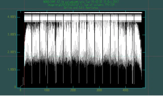
With the files sorted, the Pipeline perform three initial calibrations on the flats, which are used to both flat-field the scientific data and identify the fibers. The first step of the flat reduction is the creation of a “Mask Definition File” (MDF), which is appended (or “attached”) as a new extension to each MEF file. The MDF defines the sky coordinates of each fiber on the CCD, which allow the Pipeline to remap the 2D detector data into a 3D cube later in the reduction. To define and attach the MDF, we use the GMOS IRAF task gfreduce on the dome flat images. The task gfreduce can perform many di↵erent reduction procedures, but here we simply use it to perform the initial calibrations of the flats. The MDF defines bad fibers of the instrument, which we are required to verify by manually checking the results of the automated fiber identification. Figure 12 shows an example fiber identification window.
Figure 12. Example fiber identification window. Each “bundle” of lines is a fiber bundle consisting of 50 fibers. The numeric
ID assigned to each fiber bygfreducemust be manually checked. Incorrectly identifying the fibers can prevent proper data cube creation.
gfreducenow handles the bias subtraction and overscan subtraction and trimming of the flats. The overscan regions correspond to portions of the CCD array where light does not fall. We therefore must subtract the counts in these regions from the rest of the data and then trim them from the images.
The Pipeline repeats the above procedure of MDF attachment, overscan subtraction, and trimming for the lamp arcs. Since the arc readout speed is much faster than for the other data, we cannot use the usual bias frame to perform the bias subtraction here. Instead, we rely on the overscan levels as a rough estimate as the bias level. Finally, the Pipeline performs the bias and overscan subtraction of the science frames, as for the flats.
A.3. Bad Pixel Identification and Interpolation
A.4. Arc Extraction and Wavelength Solution Creation
The Pipeline then uses the taskgfextract to extract the arc spectra using the fiber IDs created from the flats in the first step. Now, the Pipeline calls the taskgswavelength, which creates a wavelength solution for the arc frames. This task compares each extracted spectrum to a provided list of strong emission lines and makes a polynomial fit to the data. In order to obtain a robust wavelength solution, we require that the RMS of each fit be below⇠0.09. Once the wavelength solution has been created, the Pipeline usesgftransform to apply the solution to the arc lamp images.
A.5. Quantum Efficiency Correction, Flat-Fielding, and Wavelength Solution Redo
The Pipeline now performs quantum efficiency (QE) correction on the flats usinggqecorr, and then re-extracts the BPM- and QE-corrected flat spectra. With these steps completed, the Pipeline, with gfresponse, now uses the re-extracted flats and the twilight twilight flats to create the response function which will be used to flat-field the arc lamp and science data. The response function will correct for three factors: pixel-to-pixel variations in the CCD, the wavelength-dependent efficiency of the pixels, and illumination variations.
The Pipeline usesgqecorr on the arcs, and then applies the response function created in the previous step to the now QE-corrected arcs usinggfreduce. The QE correction step changes the pixel values in the arcs, which necessitates the recreation of the wavelength solution. The wavelength solution redo is performed identically as before, using gswavelength to make the solution, and then gftransform to apply the new solution to the arcs. Figure 13 shows example wavelength-transformed science data.
Figure 13. At left: Copper-Argon (CuAr) arc lamp spectrum prior to the wavelength transformation. Note the curved
emission lines on the detector. At right: CuAr arc lamp spectrum after performing the wavelength transformation. The curved emission lines are now straight. Jagged or curved lines would indicate a bad wavelength solution. The change in image dimension between the untransformed and transformed images is the result ofgftransformstitching together the data from each chip amplifier into a single image.
A.6. Calibration of the Scientific Data
With the arcs re-transformed, the Pipeline’s processing of the calibration data has finished. The final steps of the reduction apply these calibrations to the science frames and map the 2D science data to 3D data cubes. The Pipeline first uses PyCosmic6 (Husemann et al. 2012) to identify and scrub cosmic rays from the science spectra. PyCosmic
uses the same Laplacian edge detection method as L.A. Cosmic (van Dokkum 2001), but with various extensions to
Figure 14. Example fiber spectra before (left) and after (right) cosmic ray removal. PyCosmic has e↵ectively removed the cosmic ray hits (circled in green) without harming the delicate scientific data.
the algorithm specifically tailored for use with fiber-fed spectrograph data. Whereas L.A. Cosmic frequently falsely construes the bead-like structure of the fiber data as cosmic ray hits, PyCosmic is better able to di↵erentiate the scientific data and therefore avoids destruction of strong emission lines, such as H↵. Following cosmic ray removal, the Pipeline then applies the response function and the wavelength solution to the science spectra by usinggfreduce andgftransform in succession.
A.6.1. Improper Flat-fielding and the “Two-slit” Issue
Unfortunately, observations in the Gemini program GS-2013B-Q-51 consistently lack twilight flats in one of the wavelength dithers. Therefore, we are unable to create a response function to properly flat-field any observations in the redder wavelength dither. Moreover, without proper flat-fielding, the di↵erential throughput of the pseudoslits is unaccounted for. Unfortunately, this “two-slit issue” can create a false bifurcation in the final scientific data cube (see section A.8) which may persist in the velocity fields, continuum, and line flux maps described in section 3.1.1
andsection 3.1.2. Unfortunately, we have only managed to free ourselves from the two-slit issue by excluding the red dither exposures in the 2013B semester from the data cube creation step. Consequently, these observations have SNR reduced by a factor ofp2. Insection 3.1.1, we show that consistency between GMOS IFU red dither data and SAM FP data suggest that any double nuclei and velocity field misalignment features are genuine physical features, as opposed to calibration e↵ects.
A.7. Sky Subtraction and Flux Calibration of Science
⇠6686 ˚A ⇠6687 ˚A ⇠6688 ˚A
Figure 15. Slices of the assembled data cube forrf0266 sampled at three points on the redshifted H↵line suggest complex
kinematics. We later use the shape and position of this line to extract a velocity map of the galaxy from the data cube. See
section 3.1.1.
A.8. Data Cube Creation and Mosaicking
At this point in the reduction, the Pipeline resamples the science spectra into data cubes usinggfcube. This step produces a data cubes for every science exposure. For blue nugget observations, there are generally four science exposures (two spatial and two spectral o↵sets). The Pipeline then combines the separate data cubes into a single, final cube. To perform this step, the Pipeline uses the PyFu package7 written by Gemini sta↵member James Turner.
The actual merging of the cubes is performed in a two step process. First, the PyFu taskpyfalign makes a centroid fit over the brightest feature in each wavelength-summed cube and calculates the spatial o↵sets of the centroid in each region. With the spatial o↵sets quantified, the pyfmosaic task resamples the cubes onto a common grid and then co-adds them. Any bad pixels noted in the data quality extension of the MEF are ignored in this step.
A.9. WCS Creation
Finally, the Pipeline creates a World Coordinate Solution (WCS) for the merged data cube. The known pixel scale of the scientific data and rotation✓ of the final acquisition image are used to calculate the FITS CD matrix given by:
0
@CD1 1 CD1 2
CD2 1 CD2 2
1 A=
0
@ cos✓ sin✓
sin✓ cos✓
1
A (A1)
The RA and DEC coordinates of the reference pixel are calculated as an o↵set, which depends on both the disperser used and the semester of the observation, from the commanded telescope pointing. However, the actual and commanded pointings vary with respect to each other by up to a few arcminutes. So while the rotation and scale of the WCS are well-determined, the WCS reference coordinate tends to be quite inaccurate. Normally, the WCS reference coordinate could be improved by calculating the o↵sets of field stars in the image, but the small field-of-view of our blue nugget observations does not contain any. To compensate for this issue, we manually change the coordinates of the reference pixels to center on the object.
REFERENCES
Aihara, H., Allende Prieto, C., An, D., et al. 2011, The Astrophysical Journal Supplement Series, 193, doi:10.1088/0067-0049/193/2/29
Allgood, B., Flores, R. A., Primack, J. R., et al. 2006, MNRAS, 367, 1781,
doi:10.1111/j.1365-2966.2006.10094.x
Bailin, J., & Steinmetz, M. 2005, ApJ, 627, 647, doi:10.1086/430397
Barro, G., Faber, S. M., P´erez-Gonz´alez, P. G., et al. 2013, ApJ, 765, doi:10.1088/0004-637X/765/2/104
Berlind, A. A., Frieman, J., Weinberg, D. H., et al. 2006, The Astrophysical Journal Supplement Series, 167, 1, doi:10.1086/508170
Bonnarel, F., Fernique, P., Bienaym´e, O., et al. 2000, Astronomy and Astrophysics Supplement Series, 143, 33, doi:10.1051/aas:2000331
Ceverino, D., Primack, J., & Dekel, A. 2015, MNRAS, 453, 408, doi:10.1093/mnras/stv1603
Chang, Y.-Y., van der Wel, A., Rix, H.-W., et al. 2013, ApJ, 773, doi:10.1088/0004-637X/773/2/149
Codis, S., Pichon, C., & Pogosyan, D. 2015, MNRAS, 452, 3369, doi:10.1093/mnras/stv1570
Colless, M., Dalton, G., Maddox, S., et al. 2001, MNRAS, 328, 1039, doi:10.1046/j.1365-8711.2001.04902.x
Damjanov, I., Zahid, H. J., Geller, M. J., & Hwang, H. S. 2015, ApJ, 815, doi:10.1088/0004-637X/815/2/104
Damjanov, I., McCarthy, P. J., Abraham, R. G., et al. 2009, ApJ, 695, 101, doi:10.1088/0004-637X/695/1/101
Dekel, A., & Burkert, A. 2014, MNRAS, 438, 1870, doi:10.1093/mnras/stt2331
Driver, S. P., Hill, D. T., Kelvin, L. S., et al. 2011, MNRAS, 413, 971, doi:10.1111/j.1365-2966.2010.18188.x
Eckert, K. D., Kannappan, S. J., Stark, D. V., et al. 2016, ApJ, 824, doi:10.3847/0004-637X/824/2/124
—. 2015, ApJ, 810, doi:10.1088/0004-637X/810/2/166
Eggen, O. J., Lynden-Bell, D., & Sandage, A. R. 1962, ApJ, 136, 748, doi:10.1086/147433
Falco, E. E., Kurtz, M. J., Geller, M. J., et al. 1999, Publications of the Astronomical Society of the Pacific, 111, 438, doi:10.1086/316343
Hambly, N. C., Collins, R. S., Cross, N. J. G., et al. 2008, MNRAS, 384, 637,
doi:10.1111/j.1365-2966.2007.12700.x
Haynes, M. P., Giovanelli, R., Martin, A. M., et al. 2011, AJ, 142, doi:10.1088/0004-6256/142/5/170
Hogg, D. W., & Lang, D. 2013, Publications of the Astronomical Society of the Pacific, 125, 719, doi:10.1086/671228
Hopkins, P. F., Cox, T. J., & Hernquist, L. 2008, ApJ, 689, doi:10.1086/592105
Hunter, J. D. 2007, Computing in Science and Engineering, 9, 90, doi:10.1109/MCSE.2007.55
Husemann, B., Kamann, S., Sandin, C., et al. 2012, A&A, 545, doi:10.1051/0004-6361/201220102
Ilbert, O., Salvato, M., Le Floc’h, E., et al. 2010, in SF2A-2010: Proceedings of the Annual meeting of the French Society of Astronomy and Astrophysics. Eds.: S. Boissier, M. Heydari- Malayeri, R. Samadi and D. Valls-Gabaud, p.355, 355
Jing, Y. P., & Suto, Y. 2002, ApJ, 574, 538, doi:10.1086/341065
Jones, D. H., Read, M. A., Saunders, W., et al. 2009, MNRAS, 399, 683,
doi:10.1111/j.1365-2966.2009.15338.x
Kannappan, S. J., Fabricant, D. G., & Franx, M. 2002, AJ, 123, 2358, doi:10.1086/339972
Kannappan, S. J., & Gawiser, E. 2007, ApJ, 657, L5, doi:10.1086/512974
Kannappan, S. J., Stark, D. V., Eckert, K. D., et al. 2013, ApJ, 777, doi:10.1088/0004-637X/777/1/42
Khochfar, S., & Silk, J. 2006, ApJ, 648, L21, doi:10.1086/507768
Laigle, C., Pichon, C., Codis, S., et al. 2015, MNRAS, 446, 2744, doi:10.1093/mnras/stu2289
Lang, D., Hogg, D. W., & Mykytyn, D. 2016, The Tractor: Probabilistic astronomical source detection and
measurement, Astrophysics Source Code Library.
http://ascl.net/1604.008
Law, D. R., Steidel, C. C., Shapley, A. E., et al. 2012, ApJ, 745, doi:10.1088/0004-637X/745/1/85
Markwardt, C. B. 2009, in Astronomical Data Analysis Software and Systems XVIII ASP Conference Series, Vol. 411, proceedings of the conference held 2-5 November 2008 at Hotel Loews Le Concorde, Qu´ebec City, QC, Canada. Edited by David A. Bohlender, Daniel Durand, and Patrick Dowler. San Francisco: Astronomical Society of the Pacific, 2009., p.251, Vol. 411, 251
McCall, M. L. 2004, AJ, 128, 2144, doi:10.1086/424933
Mendes de Oliveira, C., Amram, P., Quint, B. C., et al. 2017, MNRAS, 469, 3424, doi:10.1093/mnras/stx976
Mo↵ett, A. J., Kannappan, S. J., Berlind, A. A., et al. 2015, ApJ, 812, doi:10.1088/0004-637X/812/2/89
Morrissey, P., Conrow, T., Barlow, T. A., et al. 2007, The Astrophysical Journal Supplement Series, 173, 682, doi:10.1086/520512


![Figure 3. Left: SIFS spectrum for rs1103 displaying dominant H↵ and [OIII] emission lines typical of blue nugget spectra](https://thumb-us.123doks.com/thumbv2/123dok_us/8330597.2209777/6.918.129.801.98.343/figure-spectrum-displaying-dominant-emission-typical-nugget-spectra.webp)