Critical Analysis of Implementation of Just-In-Time in an Industry

(1)

International Journal of Research in Engineering & Applied Sciences

http://

www.euroasiapub.org

45

Critical Analysis of Implementation of Just-In-Time in an Industry

S. K. Jarial

Associate Professor

Mechanical Engineering Department

Deenbandhu Chhotu Ram University of Science & Technology, Murthal, India

Abstract

The purpose of this work is to check the status of implementation of Just-In-Time (JIT) inventory management technique in an Indian industry. And also investigate whether Just-In-Time (JIT) inventory management technique is a worthwhile approach or not to manage inventories. Some experts in the field maintain that the additional transportation costs derived from using JIT and its costs due to frequent transportation is more than offset by the reduction in inventory levels. In this study a simulation is developed using the cost structure of some parts of an automobile in an automobile company. This work results indicate that despite all the advantages of using JIT, JIT is not always the lowest cost technique.

(2)

International Journal of Research in Engineering & Applied Sciences

http://

www.euroasiapub.org

46

1. Introduction

JIT is a tool of lean manufacturing, which seeks to eliminate the ultimate source of waste; Variability, in all of its forms throughout the producing processes, from purchasing through distribution. By eliminating waste, JIT targets production with the minimum lead-time and at the lowest total cost. The JIT philosophy has its roots after World War II when the Japanese were striving to compete with the U.S. manufacturing system (also known as Mass Production). Tai sachi Ohno was the founder of this philosophy in the 1940s when he began developing a system that would enable Toyota to compete with U.S. automakers. Note that the environment dominating U.S. manufacturing over the last five decades has been based on the Material Requirements Planning (MRP) formalized by Joseph Orlicky, Oliver Wight, and George Plossl. In an MRP environment, planning is performed based on the independent (customers‟) demand, in an almost JIT basis. However, shop floor control is performed based on a push philosophy in which manufacturing orders are introduced in the system and pushed through production. This is the fundamental difference between JIT and MRP.According to Ohno, JIT rests on two pillars:

1. Just-in-time as it is described in the following chapters and

(3)

International Journal of Research in Engineering & Applied Sciences

http://

www.euroasiapub.org

47

2. Literature Review

Guido Nassimbeni (1995) analyses the intensity and nature of the relationship between the principal operational Just-In-Time purchasing practices. Norio Watanabe and Shusaku Hiraki (1996) consider a multi-stage multi-product production, inventory and transportation system including lot production processes and develop a goal programming model for a pull type ordering system based on the concept of a Just-In-Time (JIT) production system. Knut Richter (1996) an EOQ model is studied in which the stationary demand can be satisfied by newly made products and repaired used products. A. Gunasekran and J. Lyu (1997) implement JIT in a small company in Taiwan that produces different kinds of lamps such as rear combination lamps and front turn signal lamps. Richard Ehrhardt (1998) formulated a variety of models for studying the trade -off between finished goods inventory costs and JIT manufacturing schedule stability. Mohamad Y. Jaber, Maurice Bonney (1999) surveys work that deals with the effect of learning on the lot-size problem. It also explores the possibility of incorporating some of the ideas adapted by JIT to such models. Yan Donga, Craig R. Carter, Martin E. Dresner (2000) they developed a model and tested to determine whether the use of JIT purchasing reduces logistics costs for both suppliers and buyers. The results indicate that JIT purchasing directly reduces costs only for buyers. Vikas Kumar, Dixit Garg and N.P Mehta (2004) examine the implementation of JIT based managerial philosophy of Indian industries. Specifically JIT elements, JIT benefits and reasons for slow implementation of JIT in Indian industries are investigated through a survey. Low Sui Pheng and Wu Min (2005) Implementing just-in-time (JIT) management in the ready mixed concrete (RMC) industry seems viable. Rajeev N (2008)provide a guideline for entrepreneurs in enhancing their IM performance, as it presents the results of a survey based study carried out for machine tool Small and Medium Enterprises (SMEs) in Bangalore. Yufang Chiu (2009) proposes an inventory model that considers the defect rate to conform the real production environment. Manoj P K (2011) JIT implementation in KAMCO, an agro machinery manufacturing company based in Kerala state of Indian union.

3. Inventories Costs

a. Ordering Costs

(4)

International Journal of Research in Engineering & Applied Sciences

http://

www.euroasiapub.org

48

b. Holding Costs

Holding costs are the costs of having inventories of material on hand to distribute to meet customer demand. SPD department expresses this expense as a percentage of the value of average on-hand inventory during annual operation. It is assumed that this cost is linear due to the constant holding cost rate applied over the average inventory figure. Holding Cost Rate = Time Value of Money 10%, Warehousing 2%, Obsolescence 10%, Theft and Shrinkage 3% Total = 25% of unit price per year

4. Economic Order Quantity Model

To help solve the problems of inventory, it is necessary to build mathematical models which describe the inventory situation. Since it is never possible to represent the real world with total accuracy, approximations and simplifications must be made during the model-building process. The two fundamental questions faced by any traditional inventory system are when should an order be placed and what quantity should be ordered. To answer the second question, the Inventory Management System use some form of the Economic Order Quantity (EOQ) to determine the size of the reorder quantity. Economic order quantity model was derived originally by Harris Wilson in 1915.This model is also known as deterministic model. EOQ applies only when demand for a product is constant over the year. EOQ is the quantity to order, so that ordering cost + holding cost finds its minimum.

Total Annual cost, (TAC) = Purchase cost + Ordering cost +holding cost

𝑇𝐴𝐶 𝑄 = 𝐷𝑃 +𝐷𝐶

𝑄 +

𝑄𝐻 2

Where: D = Annual demand in units, P = Purchase cost of an item, C = Ordering cost per order, H = Holding cost per unit per year, Q = Lot size or order quantity in units,

𝐷𝐶

𝑄 =

𝑄𝐻 2

𝑄2₌2𝐷𝐶

𝐻

𝑄∗₌2𝐷𝐶

𝐻

𝑄∗₌2 × 𝐴𝑛𝑛𝑢𝑎𝑙 𝐷𝑒𝑚𝑎𝑛𝑑 × 𝑂𝑟𝑑𝑒𝑟𝑖𝑛𝑔 𝐶𝑜𝑠𝑡

(5)

International Journal of Research in Engineering & Applied Sciences

http://

www.euroasiapub.org

49

5. Analysis and Results

This study focuses on a set of ready-to-issue tractor parts. These items are consumable parts. Table 5.1 shows a sample of the items that are the focus of this study. The data are collected from Merchandiser of SPD (Spare part Division) of the company. We have select 21 parts of tractor for this study.

Table 5.1 Selected Parts with Annual Demand and Unit Price

Sr. No.

Part No. Part Description Annual Demand (D)

Unit Price(Rs.)

1 99272001 FAN 2000 258.66

2 99991770 FUEL PIPE FILTER ASSY. TO

F.I.P

3500 57.65

3 99272006 RECOVERY BOTTLE 2500 74.87

4 99991705 FILTER ELEMENT PRIMARY 12000 32.98

5 99991706 FILTER ELEMENT

SECONDARY

12000 28.09

6 99272003 ENGINE V-BELT (AV15×1125) 1000 94.7

7 99272009 OIL PRESSURE SWITCH 4000 100.28

8 99359056 GEAR SHIFTER LEVER 600 259.23

9 99358024 FIXED GEAR Z-24 1200 476.37

10 99352516 SPACER 16.5mm 350 36.88

11 99359060 GEAR SHIFTER ROD (2nd) 500 101.92

12 99359063 GEAR SHIFTER FORK (2nd) 300 234.06

13 99352524 SPACER (GEAR Z-24) 450 77.36

14 99357024 SLIDING GEAR Z-24 (M) 550 562.69

15 99991707 HYDRAULIC FILTER

(K-SERIES)

15000 154.98

16 99251075 FRONT WHEEL RIM ASSY.

(5.50F)

120 1845.91

17 99251077 FRONT TYRE 7.50"×16"-GYT 90 6384.47

18 99251057 BUMPER ASSY. 150 2188.83

19 99252025 BONNET ASSY. 150 2662.5

20 99657015 FENDER RIGHT

(13.6×28)-OLD

250 2471.74

(6)

International Journal of Research in Engineering & Applied Sciences

http://

www.euroasiapub.org

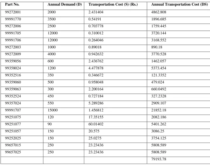
50 Table 5.2 shows that the traditional inventory management method would incur a total annual holding cost of Rs. 47421.04 for the 21 items examined. Table 5.3 shows that the transportation costs for the same group of items being managed under JIT would result in a total annual transportation cost of Rs. 79193.78. These figures indicate that a further analysis should be conducted in order to decide which technique is the more appropriate.

Table 5.2 Annual holding costs under Non JIT

Part No. Annual Demand (D)

Ordering Cost (C) (Rs.)

Holding Cost/unit per year (H) (Rs.)

Transportation Cost (S) (Rs.)

EOQ (√2DC/H)

Annual Holding Cost (HQ/2)

99272001 2000 43.97 64.665 2.431404 53 1713.62

99991770 3500 8.65 14.41 0.54191 65 468.41

99272006 2500 10.31 18.72 0.703778 53 496.01

99991705 12000 5.17 8.25 0.310012 123 507.08

99991706 12000 4.15 7.02 0.264046 120 421.35

99272003 1000 15.19 23.68 0.89018 36 426.15

99272009 4000 17.05 25.07 0.942632 74 927.59

99359056 600 41.86 64.81 2.436762 28 907.31

99358024 1200 78.65 119.09 4.477878 40 2381.85

99352516 350 6.05 9.22 0.346672 22 101.42

99359060 500 14.65 25.48 0.958048 24 305.76

99359063 300 39.79 58.52 2.200164 21 614.41

99352524 450 10.47 19.34 0.727184 23 222.41

99357024 550 90.36 140.67 5.289286 27 1899.08

99991707 15000 23.41 38.75 1.456812 135 2615.29

99251075 120 313.81 461.48 17.35155 13 2999.60

99251077 90 1085.36 1596.12 60.01402 12 9576.71

99251057 150 372.1 547.21 20.575 15 4104.06

99252025 150 452.63 665.63 25.0275 15 4992.19

99657015 250 440.2 617.94 23.23436 19 5870.38

99657025 250 440.2 617.94 23.23436 19 5870.38

47421.04

(7)

International Journal of Research in Engineering & Applied Sciences

http://

www.euroasiapub.org

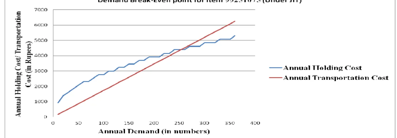
51

5.1 Graphical and Mathematical Analysis

The next step in this investigation will be a graphical and mathematical break-even point analysis of two items picked from the initial group. These items were selected randomly. They had different recommendations in Table 5.4 as far as the practice of JIT in managing those items. Table 5.5 reproduces the different annual holding and transportation costs for distinct levels of demand throughout the same year for item 99251075 (FRONT WHEEL RIM ASSY. (5.50F)). This item was selected to be under the JIT umbrella.

Table 5.3 Annual Transportation Cost of managing inventory under JIT

Part No. Annual Demand (D) Transportation Cost (S) (Rs.) Annual Transportation Cost (DS)

99272001 2000 2.431404 4862.808

99991770 3500 0.54191 1896.685

99272006 2500 0.703778 1759.445

99991705 12000 0.310012 3720.144

99991706 12000 0.264046 3168.552

99272003 1000 0.89018 890.18

99272009 4000 0.942632 3770.528

99359056 600 2.436762 1462.057

99358024 1200 4.477878 5373.454

99352516 350 0.346672 121.3352

99359060 500 0.958048 479.024

99359063 300 2.200164 660.0492

99352524 450 0.727184 327.2328

99357024 550 5.289286 2909.107

99991707 15000 1.456812 21852.18

99251075 120 17.35155 2082.186

99251077 90 60.01402 5401.262

99251057 150 20.575 3086.25

99252025 150 25.0275 3754.125

99657015 250 23.23436 5808.589

99657025 250 23.23436 5808.589

79193.78

According to the Figure above, Demand break-even-point is approximately 250. Mathematically

D = CH 2S2=

313.81 × 461.4

(8)

International Journal of Research in Engineering & Applied Sciences

http://

www.euroasiapub.org

52 The break-even point graphically and mathematically is not exactly the same due to the successive approximation built in the graphical approach.

Table 5.4 Test for JIT acceptability

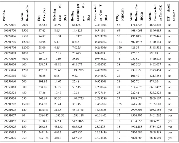
P a r t N o . A n n u a l D e m a n d (D ) U n it P r ic e (R s. ) O r d e r in g C o st (C ) (R s. ) H o ld in g C o st/ u n it p e r y e a r (H ) (R s. ) Tr a n sp o r ta ti o n C o st (S ) (R s. ) EO Q (√ 2D C /H ) A n n u a l H o ld in g C o st (H Q /2 ) A n n u a l Tr a n sp o r ta ti o n C o st (D S ) J IT sh o u ld b e u se d ?

99272001 2000 258.66 43.97 64.665 2.431404 53 1713.623 4862.808 no

99991770 3500 57.65 8.65 14.4125 0.54191 65 468.4063 1896.685 no

99272006 2500 74.87 10.31 18.7175 0.703778 53 496.0138 1759.445 no

99991705 12000 32.98 5.17 8.245 0.310012 123 507.0675 3720.144 no

99991706 12000 28.09 4.15 7.0225 0.264046 120 421.35 3168.552 no

99272003 1000 94.7 15.19 23.675 0.89018 36 426.15 890.18 no

99272009 4000 100.28 17.05 25.07 0.942632 74 927.59 3770.528 no

99359056 600 259.23 41.86 64.8075 2.436762 28 907.305 1462.057 no

99358024 1200 476.37 78.65 119.0925 4.477878 40 2381.85 5373.454 no

99352516 350 36.88 6.05 9.22 0.346672 22 101.42 121.3352 no

99359060 500 101.92 14.65 25.48 0.958048 24 305.76 479.024 no

99359063 300 234.06 39.79 58.515 2.200164 21 614.4075 660.0492 no

99352524 450 77.36 10.47 19.34 0.727184 23 222.41 327.2328 no

99357024 550 562.69 90.36 140.6725 5.289286 27 1899.079 2909.107 no

99991707 15000 154.98 23.41 38.745 1.456812 135 2615.288 21852.18 no

99251075 120 1845.91 313.81 461.4775 17.35155 13 2999.604 2082.186 yes

99251077 90 6384.47 1085.36 1596.118 60.01402 12 9576.705 5401.262 yes

99251057 150 2188.83 372.1 547.2075 20.575 15 4104.056 3086.25 yes

99252025 150 2662.5 452.63 665.625 25.0275 15 4992.188 3754.125 yes

99657015 250 2471.74 440.2 617.935 23.23436 19 5870.383 5808.589 yes

(9)

International Journal of Research in Engineering & Applied Sciences

http://

www.euroasiapub.org

53

Table 5.5 Demand Break-even-point for the item which is under JIT 99251075 (Front Wheel

Rim Assy. (5.50F))

Annual Demand = 120, Ordering cost = 313.81, Holding cost = 461.4775, transportation cost = 17.35155.

Annual Demand EOQ=

√2*D*C/H EOQ Rounding off Annual Holding Cost= HQ/2 (Rs.) Annual Transportation Cost= DS (Rs.)

10 3.687839 4 922.96 173.5

20 5.215392 6 1384.44 347

30 6.387524 7 1615.18 520.5

40 7.375678 8 1845.92 694

50 8.246259 9 2076.66 867.5

60 9.033324 10 2307.4 1041

70 9.757105 10 2307.4 1214.5

80 10.43078 11 2538.14 1388

90 11.06352 12 2768.88 1561.5

100 11.66197 12 2768.88 1735

110 12.23118 13 2999.62 1908.5

120 12.77505 13 2999.62 2082

130 13.29669 14 3230.36 2255.5

140 13.79863 14 3230.36 2429

150 14.28294 15 3461.1 2602.5

160 14.75136 15 3461.1 2776

170 15.20535 16 3691.84 2949.5

180 15.64618 16 3691.84 3123

190 16.07492 17 3922.58 3296.5

200 16.49252 17 3922.58 3470

210 16.8998 17 3922.58 3643.5

220 17.2975 18 4153.32 3817

230 17.68625 18 4153.32 3990.5

240 18.06665 19 4384.06 4164

250 18.43919 19 4384.06 4337.5

260 18.80436 19 4384.06 4511

270 19.16257 20 4614.8 4684.5

280 19.51421 20 4614.8 4858

290 19.85962 20 4614.8 5031.5

300 20.19913 21 4845.54 5205

310 20.53302 21 4845.54 5378.5

320 20.86157 21 4845.54 5552

330 21.18502 22 5076.28 5725.5

340 21.50361 22 5076.28 5899

350 21.81755 22 5076.28 6072.5

(10)

International Journal of Research in Engineering & Applied Sciences

http://

www.euroasiapub.org

54

Fig. 5.1 Demand Break-even-point for the item which is under JIT

Table 5.6 Demand Break-even-point for the item which is under Non JIT 99352516SPACER 16.5mm

Annual Demand = 350, ordering cost = 6.05, holding cost = 9.22, transportation cost = 0.346 Annual

Demand

EOQ=√2*D*C/ H

EOQ Rounding off

Annual Holding Cost= HQ/2 (Rs.)

Annual Transportation Cost= DS (Rs.)

80 10.24642 11 50.71 28

90 10.86797 11 50.71 31.5

100 11.45585 12 55.32 35

110 12.01499 13 59.93 38.5

120 12.54925 13 59.93 42

130 13.06168 14 64.54 45.5

140 13.55474 14 64.54 49

150 14.03049 15 69.15 52.5

160 14.49063 15 69.15 56

170 14.9366 15 69.15 59.5

180 15.36963 16 73.76 63

190 15.7908 16 73.76 66.5

200 16.20101 17 78.37 70

210 16.6011 17 78.37 73.5

220 16.99177 17 78.37 77

230 17.37365 18 82.98 80.5

240 17.74732 18 82.98 84

250 18.11329 19 87.59 87.5

260 18.472 19 87.59 91

270 18.82388 19 87.59 94.5

280 19.1693 20 92.2 98

290 19.50861 20 92.2 101.5

300 19.84211 20 92.2 105

310 20.1701 21 96.81 108.5

320 20.49284 21 96.81 112

330 20.81058 21 96.81 115.5

340 21.12354 22 101.42 119

350 21.43193 22 101.42 122.5

(11)

International Journal of Research in Engineering & Applied Sciences

http://

www.euroasiapub.org

55

Fig. 5.2 Demand Break-even-point for the item under non JIT

From Figure 5.2 Demand break-even-point is approximately 230. Mathematically

D =CH 2S²=

6.05 × 9.22

2 × 0.346² = 232.97

For the item 99251075 (FRONT WHEEL RIM ASSY. 5.50F) annual demands are 120. The graphical and mathematical analysis shows that the break-even point will occur when the annual demand is over 120 units. Graph 5.1, in particular, shows that the crossing point occurs all the way to the right of the normal annual demand which is 120 units.

(12)

International Journal of Research in Engineering & Applied Sciences

http://

www.euroasiapub.org

56

Table 5.7 Demand break-even-point for all items

P a r t N o . U n it P r ic e (R s. ) A n n u a l D e m a n d (D ) O r d e r in g C o st (C ) (R s. ) H o ld in g C o st/ u n it p e r y e a r (H ) (R s. ) Tr a n sp o r ta ti o n C o st (S ) (R s. ) EO Q (√ 2D C /H ) A n n u a l H o ld in g C o st (H Q /2 ) A n n u a l Tr a n sp o r ta ti o n C o st (D S ) J IT sh o u ld b e u se d ? D e m a n d Br e a k e v e n p o in t (C H /2 S ²)

99272001 258.66 2000 43.97 64.665 2.431404 53 1713.623 4862.808 No 240.4814

99991770 57.65 3500 8.65 14.4125 0.54191 65 468.4063 1896.685 No 212.2614

99272006 74.87 2500 10.31 18.7175 0.703778 53 496.0138 1759.445 No 194.8073

99991705 32.98 12000 5.17 8.245 0.310012 123 507.0675 3720.144 No 221.7656

99991706 28.09 12000 4.15 7.0225 0.264046 120 421.35 3168.552 No 209.0021

99272003 94.7 1000 15.19 23.675 0.89018 36 426.15 890.18 No 226.9144

99272009 100.28 4000 17.05 25.07 0.942632 74 927.59 3770.528 No 240.5273

99359056 259.23 600 41.86 64.8075 2.436762 28 907.305 1462.057 No 228.438

99358024 476.37 1200 78.65 119.0925 4.477878 40 2381.85 5373.454 No 233.5655

99352516 36.88 350 6.05 9.22 0.346672 22 101.42 121.3352 No 232.0699

99359060 101.92 500 14.65 25.48 0.958048 24 305.76 479.024 No 203.3445

99359063 234.06 300 39.79 58.515 2.200164 21 614.4075 660.0492 No 240.4922

99352524 77.36 450 10.47 19.34 0.727184 23 222.41 327.2328 No 191.4629

99357024 562.69 550 90.36 140.6725 5.289286 27 1899.079 2909.107 No 227.1754

99991707 154.98 15000 23.41 38.745 1.456812 135 2615.288 21852.18 No 213.688

99251075 1845.91 120 313.81 461.4775 17.35155 13 2999.604 2082.186 Yes 240.4975

99251077 6384.47 90 1085.36 1596.118 60.01402 12 9576.705 5401.262 Yes 240.4934

99251057 2188.83 150 372.1 547.2075 20.575 15 4104.056 3086.25 Yes 240.4927

99252025 2662.5 150 452.63 665.625 25.0275 15 4992.188 3754.125 Yes 240.4961

99657015 2471.74 250 440.2 617.935 23.23436 19 5870.383 5808.589 Yes 251.9426

99657025 2471.74 250 440.2 617.935 23.23436 19 5870.383 5808.589 Yes 251.9426

47421.04 79193.78

The majority of items which have been proposed for JIT management are materials with low demands, and very low weight. These characteristics lead to high inventory carrying costs and low transportation costs. These factors endorse just-in-time methodology as the primary inventory management technique. On the other hand, items with high demand, and high weight should have inventory carrying cost figures much less than their transportation costs: therefore, the traditional methodology is more cost beneficial. Each item has different parameters that influence the holding cost and transportation cost calculations as noted throughout this research. For example, the majority of those items elected for JIT show the profile of:

 Low demand (less than 250 units per year)  High unit price

In contrast, the items rejected for JIT:  High transportation cost

(13)

International Journal of Research in Engineering & Applied Sciences

http://

www.euroasiapub.org

57

6. Conclusions and Recommendations

1. JIT is the most appropriate technique for a particular set of items, after a thorough cost analysis, JIT inventory management techniques result in cost savings and add value to the final product. Hence, when the cost analysis indicates savings under a JIT environment, such techniques should be definitely adopted.

2. JIT is not always the minimum cost approach when considering a wide range of items. Hence, the cost elements under each technique should be delineated as the first step in the decision making process.

3. An item by item analysis may lead to a different diagnosis than an analysis performed for the entire group of items being managed. Therefore, a comparison between carrying costs and transportation costs should be performed on an individual item basis.

4. A graphical and mathematical break-even analysis is an excellent tool in assuring the appropriateness decision between the two techniques. Therefore, the trade-off analysis using the break-even point between the major cost drivers for each technique should be used as a filter to take advantage of the full benefits associated with JIT.

5. Inventory managers should develop the costs associated with each technique and develop a trade-off methodology, on an individual item basis. This should determine the approach that is the most suitable for each item. This is done in the context of the firm's operation, according to the company's cost structure and the demand level for each item.

References

1.

Guido Nassimbeni “Factors underlying operational JIT purchasing practices: Results of an empirical

research” Int. J. Production Economics 42, 275-288 (1995).

2.

Knut Richter “The extended EOQ repair and waste disposal model” Int. J. Production Economics 45,

443-447 (1996).

3.

Norio Watanabe and Norio Watanabe “An approximate solution to a JIT-based ordering system” Published by Elsevier Science Ltd. Printed in Great Britain Vol 31, No. 3/4, pp. 565 - 569, 1996.

4.

A. Gunasekran and J. Lyu “Implementation of JIT in a small company: a case study” vol. 8, no. 4,

406-412, (1997).

5.

Richard Ehrhardt “Finished goods management for JIT production: new mode is for analysis” VOL. 11, NO. 3, 217 ± 225, (1998).

6.

Mohamad Y. Jaber, Maurice Bonney “The economic manufacture/order quantity (EMQ/EOQ) and the learning curve: Past, present, and future” Int. J. Production Economics 59, 93-102 (1999).

(14)

International Journal of Research in Engineering & Applied Sciences

http://

www.euroasiapub.org

58

8.

Vikas Kumar, Dixit Garg and N.P Mehta “JIT practices in Indian context: a survey” vol. 63, pp. 655-662 (2004).

9.

Low Sui Pheng and Wu Min “Just-in-time management in the ready mixed concrete industries of Chongqing, China and Singapore” 23, 815–829 (2005).

10.

Rajeev N “Do inventory management practices affect economic performance? An empirical

evaluation of the machine tool SMEs in Bangalore” Vol. 3 No. 4, pp. 312-320 (2008).

11.

Yufang Chiu “Optimal JIT Production and Delivery Lot Size Model That Considers Vendor Reworking Process and Variable Setup Cost” Vol. 26, No. 2 (2009).