Veri
fi
cation of Complex Real-time
Systems Using Rewriting Logic
Mustapha Bourahla
Computer Science Department, University of Biskra, Algeria
This paper presents a method for model checking dense complex real-time systems. This approach is imple-mented at the meta level of the Rewriting Logic system Maude. The dense complex real-time system is specified using a syntax which has the semantics of timed automata and the property is specified with the temporal logic TLTL (Timed LTL). The well known timed automata model checkers Kronos and Uppaal only support TCTL model checking (a very limited fragment in the case of Uppaal). Specification of the TLTL property is reduced to LTL and its temporal constraints are captured in a new timed automaton. This timed automaton will be composed with the original timed automaton repre-senting the semantics of the complex real-time system under analysis. Then, the product-timed automaton will be abstracted using partition refinement of state space based on strong bi-simulation. The result is an untimed automaton modulo the TLTL property which represents an equivalent finite state system to be model-checked using Maude LTL model checking. This approach is successfully tested on industrial designs.
Keywords: complex real-time systems, rewriting logic, Maude LTL model checking, timed automaton, strong bi-simulation, partition refinement
1. Introduction
Many formal frameworks that have been pro-posed to reason about complex real-time sys-tems are based on timed automata [2]. These automata are equipped with clocks, variables used to measure time, ranging over the non negative real numbers(R+). Consequently, the state space is infinite and cannot be explicitly represented by enumerating all states. Among the different description languages for specify-ing real-time requirements, we are particularly interested in the temporal logic TLTL[16, 28]. Real-time model checking techniques based on partition refinement [30, 33] build a symbolic
state space that is as coarse as possible. Start-ing from some (implicit) initial partition, the partition is iteratively refined until the verifica-tion problem can be decided.
In this paper, we have augmented the LTL syn-tax used by Maude LTL model-checker[17]by operators to specify TLTL properties. Then, we have proposed a reduction technique from TLTL model-checking to LTL model-checking. This reduction will help us to analyze our sys-tem using Maude LTL model checker. Given a complex real-time system specification, a writ-ten parser with Maude [12, 13], will generate an equivalent timed automatonA. For a TLTL property specificationψ, we construct an equiv-alent LTL formulaϕ and a new timed automa-ton capturing its temporal behavior. Then, the captured behavior will be composed with the original timed automaton. This is noted byA+. We prove that A satisfiesψ if and only if A+ satisfiesϕ.
In this paper we have defined an equivalence re-lation based on strong bi-simure-lation[24], which is used by our algorithm to generate the quo-tient graph. Each edge in the timed automaton represents a discrete transition which has infor-mation concerning the source and target states, the enabling condition and the set of clocks to be reset after making this transition. Initially, the timed automaton represents the states of com-plex timed system as blocks (zones) of states
(also called symbolic states). We call this the initial partition of states. We refine any source block of states if there is an outgoing edge with an enabling condition (which is a constraint) formula different fromtrue, using the invariant of the block of states and the enabling condi-tion of this transicondi-tion. The produced sub-blocks represent classes of equivalent states where each sub-block has new invariant that either satisfies or does not satisfy the enabling condition. The refinement process will terminate if there is no block of states to be refined.
1.1. Related work
While LTL model checking is PSPACE com-plete, the TLTL model checking is undecidable
[5]. To our knowledge, it doesn’t exist until now a tool for TLTL model checking. How-ever, there are different techniques [6, 22] us-ing TLTL for the diagnosis of reactive systems and runtime verification. The problem is less severe in the case of branching-time timed log-ics, where TCTL model checking is PSPACE complete[4, 1] (whereas CTL model checking is possible in polynomial time). In contrast to TLTL model checking, there are industrial tools for TCTL model checking(KRONOS and UP-PAAL)used successfully.
In our previous work [10], an approach is pro-posed to reduce TCTL model checking to CTL model checking. This approach is implemented and tested using the SMV tool. Another simi-lar work can be found in[8], where the model checking is based on the on-the-fly exploration of a simulation graph. The simulation graph is the graph reachable, generated from the region graph[1] and from an initial region. A region is a set of states with the same location and a convex set of clock valuations. This forward-reachability approach is used in tools such as
KRONOS [15] and UPPAAL [23]. Thus, be-cause the nodes in the simulation graph are re-gion sets and only discrete transitions are ex-plicit, while time passes implicitly inside the nodes, the simulation graph is much smaller than the region graph. The simulation graph is used to solve the model checking problem for a proposed automata-based branching-time tem-poral logic (TECTL∗∃). The on-the-fly model checking procedure consists in solving the empti-ness problem, that is, in checking whether an au-tomaton(the automaton product of the system automaton and the property automaton)has an infinite execution sequence that satisfies a given acceptance condition. In our work, the property automaton capturing the temporal constraints, is automatically generated from the TLTL specifi-cation. Our quotient graph is produced directly from the initial automaton of timed system spec-ification, which resembles the simulation graph, without passing by the region graph. On the other hand, as it has been shown in[8], the sim-ulation graph preserves only linear-time proper-ties and it is used in practice mainly for reacha-bility properties. Moreover, symbolic states in the simulation graph are not necessarily disjoint, so that this graph can be much larger than the quotient graph. The quotient graph is coarser than the initial automaton but finer, and there-fore bigger, than the initial graph. Another al-gorithm that also combines the on-the-fly and the symbolic approaches has been proposed in
refin-ing unreachable classes) is adapted to infinite state space of timed automaton. This new al-gorithm which generates a finite region graph using partitioning, uses decision procedures for computing intersection, set difference and pre-decessors of classes, and testing whether a class is empty. Also, the TCTL specification is re-duced to CTL logic extended with new atomic propositions to deal with the specification con-straints. Then, a TCTL model checker has been developed based on techniques of the clas-sic CTL model-checker. The generated region graph has size exponential in the number of clocks and the highest constant used in the def-inition of timing constraints. The other closest work is in[21], where the authors propose an ap-proach to produce a compact reachability graph from a timed automaton. In this work, a state is defined as a history: execution upto the state. It is defined as a pair(location, timed history)
instead of(location, clock valuation). A timed history is a set of pairs(transition, time) upto the location of the state. An execution is de-fined as the transitions between the states( de-fined as histories). To generate an infinite state space, the algorithm uses the notion of history equivalence(states with the same untimed his-tories are merged into an equivalence class). To generate a finite state space, a transition bisim-ulation technique(the states that have the same future behaviors are further collapsed)is used to produce equivalent classes. The resultant state space is finite and can be used to analyze real-time properties. The authors have implemented this approach and analyzed applications, where the real-time properties to be verified are ex-pressed as timed automata to be composed with the system timed automata. Other techniques are based on abstraction of the constraints spec-ified in the system and in the property, using the framework of predicate abstractions as abstract interpretation[9, 25].
The rest of the paper is organized as follows. Section 2 presents a background about Rewrit-ing Logic and Maude LTL Model-Checker. In Section 3, we present the semantics based on Rewriting Logic for specification of complex real-time systems and their semantics based on the formalism of timed automata. Our approach for transformation of the TLTL specifications to LTL specifications is presented in Section 4. In Section 5, we present our method for generat-ing finite bi-similar graphs of the complex timed
systems. In Section 6, we explain how to use these graphs for Maude LTL model checking and how the results can be projected back to original complex timed systems. Complexity and implementation results of our approach are presented in Section 7. At the end, a conclusion is given.
2. Rewriting Logic and Maude LTL Model-Checker
Maude specifications are executable logical the-ories in Rewriting Logic [12, 13], a logic that is a flexible logical framework for expressing a very wide range of concurrency models and distributed systems.
A term is constructed by function and constant symbols. Each term belongs to one or sev-eral sorts. Equations specify equivalent terms. Rewriting rules specify how to transform a term into another. A rewrite theory R = (Σ,E,R)
consists of equations and rewriting rules for terms. If a rewrite theory does not contain any rewriting rules, we also call it an equational the-ory(Σ,E).
In Rewriting Logic, function and constant sym-bols are declared by the keywordop. Sorts are
declared by the keyword sort. Equations are
specified by eq lhs = rhs; conditional
equa-tions are specified byceq lhs = rhs if cond.
Similarly, rewriting rules and conditional rewrit-ing rules are defined byrl [l] : lhs => rhs
andcrl [l] : lhs => rhs if cond
respecti-vely, where lis the label of the rule. The
left-hand side of equations and rewriting rules al-lows pattern matching. Since there may be sev-eral ways to match a term, applying a rewriting rule to a given term may yield multiple results. All results obtained by any of these applications are admissible in Rewriting Logic.
Two terms are equivalent if they can be reduced to the same normal form by the equations of a rewrite theory. Equations therefore define equivalence classes of terms. For any term t, we write[t]for its equivalence class. LetRbe a rewrite theory and t, t two terms in R. We write
R l [t]→[t]
In Rewriting Logic, there is a universal theory
U such that any rewrite theory R and a termt can be presented as meta-level termsRandtin
U respectively. Furthermore, we have
R l[t]→[t]⇔ U l,n[R,t]→[R,t]
iftis the n-th result obtained by applying the rewriting rule labeledltot. By the universal the-ory U, we can manipulate meta-level terms at object level. We call the feature that can repre-sent meta-level objects at object level as reflec-tion. We have used this feature during the imple-mentation of our approach. The system Maude has metalevel operators for moving between re-flection levels asupModule,upTerm,downTerm,
and others. Other operators are used to act on metalevel terms as for parsing(metaParse)and
pretty-printing(metaPrettyPrint)terms.
Since no domain-specific model of concurrency is built into the logic, the range of applica-tions that can be naturally specified is indeed very wide. Another advantage of Maude as the system specification language is that integra-tion of model checking with theorem proving techniques becomes quite seamless. The same rewrite theory R = (Σ,E,R)can be the input to the LTL model checker and to several other proving tools in the Maude environment[17]. Thus, a Maude module is a rewrite theoryR = (Σ,E,R). Fixing a distinguished sortState, the initial model TR of the rewrite theory R =
(Σ,E,R) has an underlying Kripke structure
K(R,State) given by the total binary relation extending its one-step sequential rewrites. In the framework, the Kripke structure is specified as a rewrite theory K. The states are equiva-lence classes of terms defined inK. The tran-sitions of the Kripke structure correspond to rewriting rules in K. Since the Kripke struc-ture is specified as a rewrite theory and system configurations as equivalence classes of terms, the universal theory U can be used to explore successors of the current system configuration. To the initial algebra of statesTΣ/Ewe can like-wise associate equationally-defined computable state predicates as atomic predicates for such a Kripke structure. In this way we obtain a lan-guage of LTL properties of the rewrite theory
R.
Maude supports on-the-fly LTL model check-ing [17] for initial states [t], say of sort State,
of a rewrite theoryR= (Σ,E,R)such that the set {[t] ∈ TΣ/E|R l [t] → [t]}, of all states
reachable from[t]is finite. The rewrite theoryR should satisfy reasonable executability require-ments, such as the confluence and termination of the equationsEand coherence of the rulesR relative toE.
In Maude the rewrite theoryRis specified as a module, say M. Then, given an initial state, say initof sortStateM, we can model check
differ-ent LTL properties beginning at this initial state by doing the following[17]:
• defining a new module, say CHECK-M, that
includes the modules M and the predefined
moduleMODEL-CHECKERas submodules;
• giving a subsort declaration,
subsort StateM < State .
where State is one of the key sorts in the
moduleMODEL-CHECKER;
• defining the syntax of the state predicates we wish to use by means of constants and operators of sortProp, a subsort of the sort Formula (i.e., LTL formulas) in the
mod-uleMODEL-CHECKER; we can define
parame-terless state predicates as constants of sort
Prop, and parameterized state predicates by
operators from the sorts of their parameters to thePropsort.
• defining the semantics of the state predicates by means of equations.
Once the semantics of each of the state predi-cates has been defined, we are then ready, given an initial state init, to model check any LTL
formula, say form, involving such predicates.
We do so by evaluating in Maude, the expres-sioninit |= form .Two things can then
hap-pen: if the propertyformholds, then we get the
result true; if it doesn’t, we get a
counterex-ample expressed as a finite path followed by a cycle.
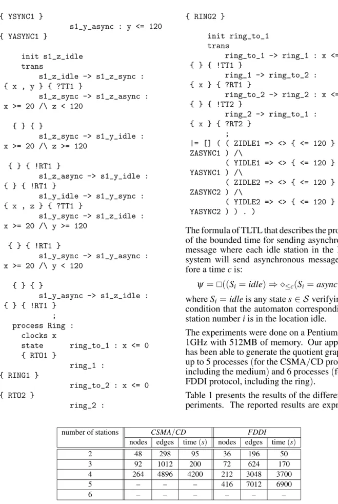
3. Complex Real-time Systems Specification
represented by a timed automaton. The pro-cesses can communicate by sending and receiv-ing messages via channels. This mechanism of communication will be used as synchroniza-tion between the different processes to compute their composition. The following is the overall system specification semantics.
op system_:’prop_;’chan_;_|=_. : Token NeTokenList
NeTokenList GProcesses Bubble -> GTProblem .
The first argument is the system identifier. A list of atomic propositions is the second argument. The third argument is a list of channels iden-tifiers. The fourth argument will represent the semantics of system processes. The last argu-ment is for the semantics of the TLTL formula. The semantics of a process is defined with the following operator. It has an identifier, a list of clock variables, a list of states, an initial state and a list of transitions.
op process_:’clocks_state_init_trans_; : Token
NeTokenList Bubble Token Bubble -> GProcess .
Clocks are real-valued variables increasing uni-formly with time. Several independent clocks may be defined for the same process. A state can have an invariant formula and a list of atomic propositions holding at this state.
op _:_{_} : Token NeTokenList NeTokenList -> GTState .
A transition is between two states(source and target, first and second argument, respectively). The transition is conditioned by a temporal con-straint. As actions, a transition can reset clocks and it can send and receive messages via the specified channels. This mechanism of sending and receiving messages will be used for syn-chronization.
op _->_:_{_}{_} : Token Token NeTokenList NeTokenList
NeTokenList -> GTTransition .
A temporal constraint has the following seman-tics.
ops True False : -> TConstraint . op _=_ : Token Time -> TConstraint . op _>_ : Token Time -> TConstraint . op _>=_ : Token Time -> TConstraint . op _<_ : Token Time -> TConstraint . op _<=_ : Token Time -> TConstraint . op _/\_ : TConstraint TConstraint ->
TConstraint [id: True] . op _\/_ : TConstraint TConstraint ->
TConstraint [id: False] .
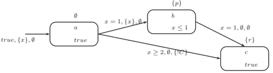
The following is an example, which has two atomic propositions,pandr. One
communica-tion channel C. This complex real-time system
is composed of one process with three states:
a, b, and c and three transitions. The
real-time specification is followed by specification of a TLTL property which can be omitted and given separately to allow the specification of different TLTL properties.
system Example : prop p r ; chan C ; process P :
clocks x state
a : { }
b : x <= 1 { p }
c : { r }
init a trans
a -> b : x = 1 { x } { } a -> c : x >= 2 { } { !C } b -> c : x = 1 { } { } ; |= True U { >= 2 } r
The semantics of a complex real-time system is represented by timed automata[2]which ex-tend the automata formalism by adding clocks. These semantics will be defined by the follow-ing two main operators. The first partial opera-tor(getSystem)is called when the parsing of a
complete specification is succeeded (the result of the parsing is a Term), to generate needed
semantics as system identifier, atomic propo-sitions, and channels identifiers. This opera-tor calls the second (solveProcesses)to
op getSystem : Term ~> TimedSystem . op solveProcesses : Term ~>
TimedAutomaton .
A timed automatonAis a tuple
Q,X,Σ,E,L1,L2,I, where:
• Qis a finite set of locations. We denote by q0∈ Qthe initial location.
• X is a finite set of clocks. A valuationv is a function that assigns a non negative real-valuev(x) ∈ R+ to each clockx ∈ X. The valuation v[X := δ] assigns the value δ to all clocks in the setX. The set of valuations is denotedVX. Forδ ∈ R+, v+δ denotes
the valuation v such that v(x) = v(x) +δ
for allx∈ X.
• Σis a finite set of labels(message channels).
• Eis a finite set of edges. Each edgee∈ E is a tupleq,θ,X,σ,q where
– q,q ∈ Q are the source and the target locations respectively,
– θ ∈ Θ is an associated clock constraint which governs the triggering of the tran-sition. It is called its enabling condition or its guard. We denote the set of con-straints over X by Θ. A constraint is defined as a conjunction of atoms of the form x ∼ c, where x ∈ X, ∼∈ {=, >, ≥, <,≤}andcis a natural constant. – X ⊆ X is the set of clocks to be reset
after making this transition.
– σ is a subset of synchronization events from the setΣ. A synchronization event is the combination of a channel name pre-ceded by the symbol ! to indicate send
event, or?for receive event.
• L1 : Q → 2AP is a function that associates
to each location a set of atomic propositions from the setAP.
• L2 : E → 2Σ is a function that associates
to each edge a set of synchronization events from the setΣ. We have two kinds of syn-chronization events(send events and receive events).
• I is a function that associates a condition
I(q)∈Θto every locationq∈ Qcalled the invariant ofq.
Figure 1 shows an example of a timed automa-ton representing the semantics of the example above. AP = {p,r} and Q = {a,b,c}. A state ofAis a pairq,v ∈ Q × VX such that v satisfies I(q). The initial state is the pair
q0,v0 such that v0(x) = 0 for all x ∈ X.
Let S denote the set of states of A. We will refer to L1(s) by L1(q), for all s ∈ S, where
s = q,v. The set S can be partitioned to zones(symbolic states). A zonez= (q,Vz)is
a set of states fromSwhich are associated with the same discrete stateq∈ Qand a convex set of valuationsVz = {v | ∃q,v ∈ S}. The state
of a timed system can be changed through an edge that changes the location and resets some of the clocks (discrete transition), or by letting time pass without changing the location (time transition).
Let e = q,θ,X,σ,q ∈ E be an edge. The stateq,v has a discrete transition toq,v, denoted q,v → d q,v, if v satisfiesθ and v = v[X := 0] (we should note that the set of valuations respecting θ is always in the set of valuations respectingI(q)). Letδ ∈ R+. The stateq,v has a time transition toq,v+δ, denotedq,v → τ q,v+δ, if for allδ ≤δ,
v+δsatisfies the invariantI(q).
For timed automata, we label each discrete tran-sition with a label (or an action) a. The label is composed of a temporal constraint to exe-cute the transition when it holds and an ac-tion of resetting clocks. The time transiac-tions
true,{x},∅
∅
a true
x= 1,{x},∅
x≥2,∅,{!C} {p}
b
x≤1 x= 1,∅,∅ {r}
c true
have a particular label namedτ denoting time elapse which is considered as an internal or hid-den action. Let A be the set of actions and Aτ =A∪ {τ}. We noteM= (S,Aτ,T,s0,L)
the labeled transition system of A (its seman-tics),Sis the set of reachable states froms0with
respect toT. L :S →2AP andL(s) = L1(q),
for eachs∈q. T ⊆ S ×Aτ×Sthe(discrete or time)transition relation and s0the initial state.
For each labela and each state s, we consider the image set Ta(s) = {s ∈ S | (s,a,s) ∈
T }. We extend this notation for sets of states:
Ta(B) = ∪{Ta(s) | s ∈ B}. T−1 denotes the
inverse relation.
A run r ofMis an infinite sequence of states and transitions. We denote R the set of runs ofM. A run is divergent if ∞i=0δi (the sum of all delays δi on this run) diverges. We de-note R∞ the set of divergent runs of M. In the following, we will consider timed automata with only divergent runs(if the automaton has non-divergent runs, called also zeno runs, it is possible to restrict the behavior to divergent runs
[19]).
A complex real-time system is composed of many processes using the operator Compose.
Their different timed automata will be com-posed to construct the timed automaton of the overall complex real-time system.
op Compose : TimedAutomaton TimedAutomaton ->
TimedAutomaton .
The parallel composition of two timed automata
()is defined as follows. LetAibe Qi, Xi, Σi,
Ei, L1i, L2i, Ii, for i = 1,2. We assume
that Q1 ∩ Q2 = ∅ and X1 ∩ X2 = ∅. The
product-timed automaton A = A1 A2 =
Q,X,Σ,E,L1,L2,I is such that: Q=Q 1×
Q2,X =X1∪ X2,Σ=Σ1∪Σ2,I(q1,q2) =
I1(q1) ∧ I2(q2), L1(q1,q2) = L11(q1) ∪
L1
2(q2), L2 is defined during the composition
of edges. The set E of edges is obtained as follows.
1. for all q1,θ1,X1,σ1,q1 ∈ E1 and
q2,θ2,X2,σ2,q2 ∈ E2:
• ifreceive(σ1)
⊆ send(σ2) ∧receive(σ2) ⊆ send(σ1)
then E includes(q1,q2),θ1∧θ2,X1 ∪
X2,send(σ1∪σ2),(q1,q2).
• ifreceive(σ1)⊆send(σ2)∧(receive(σ2) =∅∨receive(σ2)⊆send(σ1))thenE in-cludes(q1,q2),θ1,X1,send(σ1∪σ2)∪
receive(σ2)\send(σ1),(q1,q2).
• ifreceive(σ2)⊆send(σ1)∧(receive(σ1) =∅∨receive(σ1)⊆send(σ2))thenE in-cludes(q1,q2),θ2,X2,send(σ1∪σ2)∪
receive(σ1)\send(σ2),(q1,q2).
2. for allq1,θ1,X1,σ1,q1 ∈ E1, ifchannel
(σ1) ∈ Σ1∩Σ2 then∀q2 ∈ Q2, E includes
(q1,q2),θ1,X1,σ1,(q1,q2).
3. for allq2,θ2,X2,σ2,q2 ∈ E2, ifchannel
(σ2) ∈ Σ1∩Σ2 then∀q1 ∈ Q1, E includes
(q1,q2),θ2,X2,σ2,(q1,q2).
receive(σ) and send(σ) are used to extract channel names used by receive and send events, respectively. channel(σ) returns the name of the communication channel used by the event
(receive or send) σ. Note that receive(∅) =
send(∅) =channel(∅) = ∅. A transition wait-ing reception of messages from transitions in other processes via defined transmission chan-nels, will be composed only with those transi-tions delivering these messages.
The first case of (1) indicates that the receive events on both transitions are sent mutually by these two transitions. The second case of (1)
indicates that the receive events of the first tran-sition are all sent by the second trantran-sition, but the receive events of the second are empty or not all sent by the first transition. The third condition of(1)is the symmetry of the second. The cases(2)and(3)are for automata not shar-ing communication channels. The composition of two automata without synchronization events equals to their Cartesian product. This compo-sition of timed automata representing different processes of a system, terminates by producing one timed automaton without synchronization events. The produced system timed automaton will be composed with the property timed au-tomaton generated from the TLTL specification.
4. Transformation of TLTL Specifications
linear time logic LTL [16, 3, 28]. This exten-sion either augments temporal operators with time bounds, or uses reset quantifiers. We use a version of TLTL with time bounds.
Maude LTL model checker [17] provides the common LTL operators U, W, R, , and O, written as until, until weak, releases, al-ways, eventually, and next in addition to the well known set of Boolean operators : ¬,∧,∨,
⇒and ⇔. The formulas ϕ of the linear tem-poral logic LTL are defined inductively by the grammar:
ϕ ::= true | p | ¬ϕ | ϕ ∧ϕ | ϕUϕ | ϕWϕ |
ϕRϕ |ϕ | ϕ |Oϕ.
Wherep ∈ AP is an atomic proposition. The LTL semantics over a labeled transition system, are defined using the satisfaction relation, de-noted bys|=ϕ, on the syntax ofϕ:
• s|=true
• s|=piffp∈ L(s) • s|=¬ϕiffs|=ϕ
• s|=ϕ∧ϕiffs|=ϕ∧s|=ϕ
• s |= ϕUϕ iff ∀r ∈ R∞ andr(0) = s,∃i
andr(i)|=ϕand∀j<i.r(j)|=ϕ • s|=ϕWϕiffs|=ϕUϕ∨s|=ϕ • s|=ϕRϕiffs|=ϕWϕ
• s |= ϕ iff ∀r ∈ R∞ and s = r(0),∀i ≥
0.r(i)|=ϕ
• s|=ϕiffs|=trueUϕ
• s |=Oϕ iff∀r ∈ R∞ andr(0) = s,r(1) |=
ϕ
The added TLTL (Timed LTL) operators are: O∼cϕ states that the next occurrence of ϕ is within the time bounds∼c. ϕU∼cψ states that
ϕis true until the next occurrence ofψ, and that this occurrence ofψ is within the time bounds
∼ c. ∼cϕ states that ϕ must always be true
within the time bounds∼ c. ∼cϕ states that
ϕ must be true at some point within the time bounds ∼ c, where ∼∈ {=, >,≥, <,≤} and c∈N (Nis the set of natural numbers).
The formulas ψ of the timed linear temporal logic TLTL are defined inductively by the gram-mar:
ψ ::=ϕ |O∼cψ |ψU∼cψ |∼cψ | ∼cψ.
Where ϕ is an LTL formula. The formulas of TLTL are interpreted over the set of states of a timed automaton represented by a transition systemM. Letq,v ∈ Sbe a state reachable in M and let a TLTL-formula ψ. The satis-faction relation, denoted by q,v |=M ψ, is defined inductively on the syntax ofψ:
• q,v |=Mϕ Its semantics is defined using the semantics of the logic LTL.
• q,v |=M O∼cψ iff∀r ∈ R∞ andr(0) =
q,v,∃i.Σj≤iδj ∼ c and r(i) |=M ψ and ∀j<i.r(j)|=Mψ
• q,v |=M ψU
∼cψ iff ∀r ∈ R∞ and
r(0) = q,v,∃i.Σj≤iδj ∼ c andr(i) |=M
ψand∀j<i.r(j)|=Mψif∼∈ {=,≥, >}
thenr(j)|=Mψ
• q,v |=M∼cψiffq,v |=M TrueU∼cψ
• q,v |=M ∼cψ iff∀r ∈ R∞andr(0) =
q,v,∃i.Σj≤iδj ∼cand∀j∼i,r(j)|=Mψ
We augmented the LTL syntax used by Maude LTL model-checker by the following operators to specify TLTL properties.
op O’{=_}_ : Time Formula -> Formula . op O’{>_}_ : Time Formula -> Formula . op O’{>=_}_ : Time Formula -> Formula . op O’{<_}_ : Time Formula -> Formula . op O’{<=_}_ : Time Formula -> Formula . op _U’{=_}_ : Formula Time Formula -> Formula .
op _U’{>_}_ : Formula Time Formula -> Formula .
op _U’{>=_}_ : Formula Time Formula -> Formula .
op _U’{<_}_ : Formula Time Formula -> Formula .
op _U’{<=_}_ : Formula Time Formula -> Formula .
Our objective is to transform a TLTL formula
ψ to an LTL formulaϕ. Any TLTL formulaψ
will introduce a new set of specification clocks
Xψ. This set of specification clocks does not
control the behavior of any system under con-sideration. The transformation process reduces the TLTL formulaψ recursively by decompos-ing ψ. At the end, it generates an equivalent LTL formulaϕand a timed automatonAψ,
cap-turing the timed behavior specified in the TLTL formulaψ. If the formula does not contain tem-poral constraint(it is already an LTL formula), the transformation process returns this formula and an empty timed automaton.
On the other hand, if the TLTL formula con-tains temporal constraints, these can be of one of the forms presented below. The constructed timed automaton Aψ, is almost the same for
all the forms which have a set of one clock variable Xψ = {z}, two discrete statesQψ =
{qψ0,qψ1} with invariants z ≤ c and true re-spectively(these two discrete states are labeled according to the formula), and one edgeEψ = {(qψ0,z = c,∅or {z},∅,qψ1)}. This timed au-tomaton will be composed(using the operator
TComposeof linear composition)with the
prod-uct of the two timed automata Aψ and Aψ constructed by the recursive call to the functions
Transform(ψ,Pr)andTransform(ψ,Pr)
re-spectively. The second argument is used to label one of the two discrete states(Qψ ={qψ0,qψ1}). The following is an example for transformation of the formulas of the formϕU≥cψ andϕU≤cψ
respectively.
op Transform : Formula Id -> AutomatonFormula .
ceq Transform(F U { >= T } F’, Pr) = {
TCompose(getCapAutomaton (AF1:AutomatonFormula),
TCompose(
("U" : { "z" } ; { "q1" } ; { ("q1" : "z" <= T { empty }) ,
("q2" : True { Pr }) } ;
{ ("q1" -> "q2" : "z" = T { empty } { empty }) }
),
getCapAutomaton
(AF2:AutomatonFormula))) ; (getTrsFormula
(AF1:AutomatonFormula) /\
~ getTrsFormula
(AF2:AutomatonFormula)) U (getTrsFormula
(AF2:AutomatonFormula) /\ Prop(qid(Pr)))
}
if AF1:AutomatonFormula := Transform(F, Pr + "1") /\
AF2:AutomatonFormula := Transform(F’, Pr + "2") .
ceq Transform(F U { <= T } F’, Pr) = {
TCompose(getCapAutomaton (AF1:AutomatonFormula),
TCompose(
("U" : { "z" } ; { "q1" } ; { ("q1" : "z" <= T { Pr }) ,
("q2" : True { empty }) } ;
{ ("q1" -> "q2" : "z" = T { empty } { empty }) }
),
getCapAutomaton
(AF2:AutomatonFormula))) ; (getTrsFormula
(AF1:AutomatonFormula) /\ Prop(qid(Pr))) U
(getTrsFormula
(AF2:AutomatonFormula)) } if AF1:AutomatonFormula := Transform(F, Pr + "1") /\
AF2:AutomatonFormula := Transform(F’, Pr + "2") .
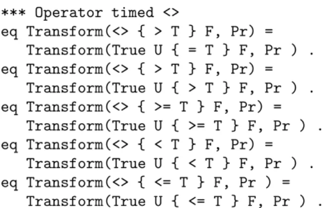
The transformations for the other TLTL opera-tors are coded almost by the same manner. The formulas using the timed operatorsOandare converted to equivalent formulas before trans-formation as follows.
*** Operator timed O
eq Transform(O { = T } F, Pr) = Transform(([] { < T } (~ F)) /\
(True U { <= T } F), Pr) . eq Transform(O { > T } F, Pr) =
Transform((~ F) /\ ((~ F) U { > T } F), Pr) .
eq Transform(O { >= T } F, Pr) =
Transform((~ F) /\ ((~ F) U { >= T } F), Pr) .
eq Transform(O { < T } F, Pr) =
Transform((~ F) U { < T } F, Pr) . eq Transform(O { <= T } F, Pr) =
*** Operator timed <>
eq Transform(<> { > T } F, Pr) = Transform(True U { = T } F, Pr ) . eq Transform(<> { > T } F, Pr) =
Transform(True U { > T } F, Pr ) . eq Transform(<> { >= T } F, Pr) =
Transform(True U { >= T } F, Pr ) . eq Transform(<> { < T } F, Pr) =
Transform(True U { < T } F, Pr ) . eq Transform(<> { <= T } F, Pr ) =
Transform(True U { <= T } F, Pr ) .
Example 1. For the TLTL formula ψ = ≥2r
(which is equivalent to trueU≥2r), the function Transform generates the equivalent LTL
for-mulaϕ and the timed automatonAψ shown in Figure 2.
true,{z}
∅
q1
z≤2
z= 2,∅,∅
“Z”
q2
true ϕ= (¬P rop(r))U(P rop(Z)∧P rop(r))
Figure 2.Generated timed automatonAwith LTL formulaϕforψ =≥2r.
The following is the result of the Maude com-mand.
reduce in VRTS : Transform(<>{>= 2}Prop (’r), "Z") .
rewrites: 13 in -157072442571ms cpu (0ms real)
(~ rewrites/second)
result AutomatonFormula: {"U" :{"z"}; {"q1"};
{("q1" : "z" <= 2{empty}),"q2" : True{"Z"}};{"q1" -> "q2" : "z" = 2{empty}{empty}} ;
(~ Prop(’r)) U (Prop(’Z) /\ Prop(’r))}
Example 2. This is another example. Let the TLTL formulaψ = ≤2(a∧ ≤1b). The
func-tion Transform generates the equivalent LTL
formulaϕand the timed automatonAψ shown
in Figure 3.
red Transform(<> { <= 2 } (Prop(’a) /\ (<> { <= 1 }
Prop(’b))), "Z") .
reduce in VRTS : Transform(<>{<= 2}((<> {<= 1}Prop(’b))
/\ Prop(’a)), "Z") .
rewrites: 79 in -3902117295ms cpu (0ms real)
(~ rewrites/second)
result AutomatonFormula: {"UU" :{"z"}; {"q1q1"};
{("q1q1" : "z" <= 2{"Z","Z2111"}), ("q1q2" : "z" <= 2{"Z"}),("q2q1" : "z" <= 3{"Z2111"}),"q2q2" :
True{empty}};
{"q1q1" -> "q2q1" : "z" = 2{empty}{empty},
"q2q1" -> "q2q2" : "z" = 3{empty}{empty}} ;
(Prop(’Z)) U ((((Prop(’Z2111)) U (Prop(’b)))
/\ Prop(’a)))}
The constructed timed automaton Aψ will be
composed with the original timed automatonA
(A Aψ). The operator Transform is using
the operator TCompose to realize a linear
com-position(denoted by⊕)of two timed automata. It is defined to compose the constructed timed automata Aψ and Aψ, where ψ and ψ are sub-formulas of ψ, to get only one timed au-tomatonAψ with one clock variablez. Its
dif-ference from the operator is in the construc-tion of the set of edges E, which is obtained as follows. Let ei ∈ Ei of the form qi,zi =
ci,∅,∅,qi, for i = 1,2. Then, if c1 < c2,
we add e = (q1,q2),z = c1,∅,∅,(q1,q2)
to E, where I(q1,q2) = z ≤ c1. We
re-place e2 in E2 by q2,z2 = c2− c1,∅,∅,q2
and we remove e1 from E1. Else, if c2 < c1,
true,{z}
“Z”, “Z2111”
q1q1
z≤2
z= 2,∅,∅
“Z2111”
q2q1
z≤3
z= 3,∅,∅
∅
q2q2
true ϕ=P rop(Z)U((P rop(Z2111)UP rop(b))∧P rop(a))
we adde = (q1,q2),z =c2,∅,∅,(q1,q2) to
E, where I(q1,q2) = z ≤ c2. We replace
e1 inE1byq1,z1 = c1−c2,∅,∅,q1 and we
removee2 from E2. Else, e = (q1,q2),z =
c1,∅,∅,(q1,q2), whereI(q1,q2) =z ≤c1
and we removee1fromE1,e2fromE2.
This process will continue until Ei = ∅, for
i = 1,2 or one of the following two cases is satisfied. In the case where E1 = ∅ and
E2 = {q2,z2 = c2,∅,∅,q2 }, we assume
thatq1 ∈ Q1 is the discrete state without
out-going edge. Then, we add the edge e = (q1,q2),z = c2,∅,∅,(q1,q2) to E, where
I(q1,q2) = z ≤c2. In the other case where
E2 = ∅ and E1 = {q1,z1 = c1,∅,∅,q1 },
we assume that q2 ∈ Q2 is the discrete state
without outgoing edge. Then, we add the edge e = (q1,q2),z = c1,∅,∅,(q1,q2) to
E, where I(q1,q2) = z ≤ c1. At the
end, if there are discrete states in the produced timed automaton, without ingoing and outgo-ing edges, they will be removed from the set of discrete statesQ.
Theorem 1. LetMbe the transition system of the timed automaton A modeling a real-time system. If the function Transform produces
an LTL formulaϕ and a timed automatonAψ from a TLTL formulaψ, and if q,v |=M ψ
(the state q,v satisfies the TLTL formula
ψ), and q,v |=M+ ϕ (the state q,v sat-isfies the LTL formula ϕ (M+ is the tran-sition system of A+ = A Aψ)). Then,
q,v |=Mψ ⇔ q,v |=M+ ϕ
Proof. The proof proceeds by induction on the structure ofψ. The basis case whereψ is of the formϕ (an LTL formula) is immediate. In this basis caseAψ =∅; andM+ =M, this means q,v |=Mψ ⇔ q,v |=M+ ϕ.
We will prove the caseψ = ψU
≥cψ and the
other cases can be proved by the same way. Consider a state q,v in M. Assume that
q,v |=Mψ. Then, by the semantics of TLTL,
for any run r=q0,v0,q1,v1,· · ·,qi,vi,
· · · ∈ R∞withq0,v0 =q,v, where i≥ 0
such that Σi
k=0δk ≥ c and qi,vi |=M ψ,
and for all 0 ≤ j < i we have qj,vj |=M ψ∧ ¬ψ.
If the timed automaton Aψ = Aψ ⊕ {Q =
{qψ0,qψ1},X = {z},Σ = ∅,eψ = (qψ0,z =
c,∅,∅,qψ1),L1 = {L1(qψ
0) = True,L1(qψ1) =
“Z"},L2 = ∅,I = {I(qψ
0) = z ≤ c,I(qψ1) =
True}} ⊕ Aψ and the TLT formulaϕ =ϕ∧
¬ϕUϕ∧“Z"are the results ofTransform(ψ =
ψU∼cψ), where⊕is the operatorTCompose
as defined before,{Aψ,ϕ}and{Aψ,ϕ}are the results of Transform(ψ) and Transform (ψ), respectively.
By the induction hypothesis,qi,vi |=M ψ⇔ (qi,qψ),vi |=M+
ψ ϕ
(M+
ψ is the model
of A Aψ) and qj,vj |=M ψ ∧ ¬ψ ⇔
(qj,qψ),vj |=M+
ψ ϕ
∧ ¬ϕ (M+
ψ is the model ofA Aψ). It is clear from the parallel composition that (qi,qψ,qψ),vi |=M+
ψψ
ϕ and(qj,q
ψ,qψ),vj |=M+ ψψ ϕ
, where
M+ψψis the model ofA (Aψ⊕ Aψ)(⊕is the operatorTComposeas defined before).
IfM+ is the model of A Aψ, then it is clear that vi(z)≥c and using the property of parallel
composition, we have(qi,qψ,qψ,qψ1),vi
|=M+ ϕ∧“Z"(L1(qψ1) =“Z") and for all0≤ j < i we have (qj,qψ,qψ,qψ0),vj |=M+
ϕ∧ ¬ϕ. By the semantics of TLTL, we have q,v |=M+ ϕ∧ ¬ϕUϕ∧“Z".
5. Generating Bi-similar Finite System
The model of a timed automaton is an infinite transition-state system due to dense time. Then, it is not possible to perform a model checking. In this section we present our method that gen-erates a strongly bi-similar finite system based on a defined equivalence where exact delays are abstracted away while information on the dis-crete changes of the system is retained.
5.1. Strong Bi-simulation
For a labeled transition systemM= (S,Aτ,T, s0,L), a partition℘(or equivalence relation on
S)of the elements ofSis a set of disjoint blocks
{Bi | i ∈N}such that∪i∈NBi =S. Let ℘and
℘ be partitions of S. ℘ is a refinement of ℘ (℘ ℘) if and only if ∀B ∈ ℘ : ∃B ∈ ℘ : (B ⊆ B). Intuitively, two states s1 and s2 are
bi-similar if for each states1 reachable froms1
3)there is a states2, reachable from s2 by
ex-ecution of the action a such thats1 and s2 are bi-similar.
Definition 1. Given a labeled transition sys-tem M = (S,Aτ,T,s0,L), a binary relation
℘⊆ S × S is a strong bi-simulation if and only if the following conditions hold ∀(s1,s2) ∈ ℘
and∀a∈Aτ: 1. L(s1) =L(s2),
2. ∀s3(s3 = Ta(s1) ⇒ ∃s4(s4 = Ta(s2) ∧
(s3,s4)∈℘))and
3. ∀s4(s4 = Ta(s2) ⇒ ∃s3(s3 = Ta(s1) ∧
(s3,s4)∈℘)).
The set of bi-simulations onS, ordered by inclu-sion has a minimal element which is the identity relation denoted by℘0and it has a maximal
el-ement denoted by℘maxwhich is an equivalence
relation on(or a partition of)S. We will be in-terested in the maximal element which induces the smallest number of equivalence classes in terms of relation inclusion. ℘max (which is
unique) may be obtained as the limit of a de-creasing sequence of relations℘i.
Most algorithms used to solve the bi-simulation problem are based on some form of partition re-finement, i.e. they perform successive iterations in which blocks of the current partition are split into smaller blocks, until no block can be split any more. While splitting a block, states that cannot be distinguished are kept in the same block. Two states can be distinguished if one of the states allows a transition with a certain label to a state in a certain block and the other state does not have a transition with the same label to a state in the same block. This means that in our case of timed automata the time associated to a state doesn’t satisfy the temporal constraint labeling the transition.
Let℘be a partition ofS. ℘is compatible with
T (it is also called stable) if and only if the following propertyP holds:
P(℘)≡ ∀a∈Aτ :∀B,B ∈℘:
(B ⊆ T−1
a (B)∨B∩Ta−1(B) =∅).
Correctness of a partition refinement algorithm follows from two facts. First, a stable partition is a bi-simulation relation (states are equiva-lent if they are in the same block). Second,
each computed partition by the refinement of the previous one respects the propertyP.
Definition 2. Let M = (S,Aτ,T,s0,L) be a
labeled transition system and℘an equivalence relation which is a strong bi-simulation, the quotient labeled transition system denoted by
M/℘is defined as follows:M/℘= (S/℘,Aτ, T/℘,s0,L/℘), where:
• S/℘ is the set of equivalence classes noted
C,C =B⊆ S | ∀s1,s2∈B:(s1,s2)∈℘)
• ((B=Ta(B))∈ T/℘)if and only ifTa−1(B)
∩B =∅
• ∀C ∈ C :L/℘(C) =L(s), where s∈C.
• C0 = [s0]is the equivalence class of s0.
M/℘maxis the normal form ofMwith respect
to℘max. We present below the implementation
with Maude of our partition-refinement algo-rithm based on strong bi-simulation. We start from an initial partition of the state space in zones. Each time a zoneZis to be refined, it is split with respect to all its discrete successors by some edgee. We can prove that if all successors are zones, then the result of the split is also a set of zones, that is, convexity is preserved by the split operation.
5.2. Partition-refinement Algorithm
A product timed automatonA = Q,X,Σ,E, L1,L2,I can contain spurious behaviors. This
means that there are paths in the product-timed automaton that will never be executed. These spurious behaviors are due to parallel compo-sition which doesn’t predict them. Thus, it is necessary to get rid of them before the pro-cess of(time abstraction)partition refinement. If not, these spurious behaviors will be part of the overall system behavior and will yield false negative counterexamples. There are tech-niques to remove spurious behaviors. We have used simulation of the product-timed automa-ton. The unfired transitions during simula-tion will be removed from the timed automa-ton. The result of simulation is a timed graph
G = Q,X,E,L,I, where E is the set of edges without event labels, andLis defined ex-actly as L1. Let e = q,θ,X,q ∈ E be an
The objective of refinement is to abstract the quantitative aspect of time needed to measure the constraintθ. So, this block of states(zone) is refined into sub-zones. The invariant of one of these sub-zones satisfies the constraintθ. But, the invariants of the other sub-zones don’t sat-isfy this constraint. This process of refinement will continue until there are no blocks to refine. The operators over temporal constraints, used in the algorithm of partition refinement are defined as follows.
1. Var(θ) is the set of clock variables in the
formulaθ.
2. With(θ, x)is the constraint θ reduced to a
constraint defined only on the clock variable x (e.g. With(x = 1∧y < 2∧z ≤ 3, x)
≡x=1)
3. Without(θ,x)is the constraintθ reduced to
a constraint defined without the clock vari-ablex(e.g. Without(x=1∧y<2∧z≤3,
x)≡y<2∧z≤3)
4. &is the intersection operator (e.g. x ≤ 2 &
x ≥2 ≡ x =2). θ1 &θ2 = ∅ifVar(θ1)∩ Var(θ2)=∅.
5. \is the set difference operator(e.g. x≤2\
x =1 ≡ x <1∨(x >1∧x≤ 2), it is not convex).
6. floor(θ)if θ is convex, then this operator
will return θ itself, else it returns the con-straint representing the lower convex valua-tions. The constraint θ is defined on one clock variable (e.g floor(x < 1 ∨ (x >
1∧x≤2))≡x<1).
7. ceil(θ) if θ is convex, then this operator
will return ∅, else it returns the constraint representing the upper convex valuations. The constraintθis defined on one clock vari-able (e.g ceil(x < 1∨(x > 1∧x ≤ 2))
≡x>1∧x≤2).
Our defined Maude operatorsplitsplits a zone
that is a source of an edge e = q,θ,X,q, taken arbitrarily from the set E of the current partition, where θ = true. The refinement
(splitting)is based on a clock variablex taken also arbitrarily from the set of clock variables in the constraintθ. The zone is split into at most three sub-zones. These sub-zones have the same locationq, but with different invariants. Their union equals toI(q). Because their invariants
are different and for algorithm simplicity, we will denote their locationqdifferently to distin-guish them. This will not have any effect on the algorithm results.
The first sub-zeno (with discrete stateqx) has
the invariantI(qx) =With(θ,x)∧Without(I(q),
x)and an outgoing edgeqx,Without(θ,x),∅,q.
Iffloor(With(I(q),x)\With(θ,x))=∅, we
have a second sub-zone with a discrete stateql
with an invariantI(ql) =floor(With(I(q),x)
\ With(θ,x)) ∧ Without(I(q),x). This
sub-zone has an outgoing edgeql,true,∅,qx.
Ifceil(With(I(q),x)\With(θ,x))=∅, then
we have a third sub-zone with a discrete state qu and an invariant I(qu) = ceil(With(I(q),
x) \ With(θ, x)) ∧ Without(I(q), x). This
sub-zone has an ingoing edgeqx,true,∅,qu.
The three new sub-zones will be marked by the same set of atomic propositionsL(q).
At the end of this iteration, the edgee and the zoneZwill be removed and replaced by the new edges and the new sub-zones. The other outgo-ing and incomoutgo-ing edges from and to the zoneZ will be updated according to the new partition. The non-zenoness of the timed automaton and the convexity of its constraints guarantee that the produced partition has zones preserving the convexity and the non-zenoness. Moreover, the algorithm terminates.
5.3. Quotient Graph
The partition-refinement algorithm generates a stable partition℘maxwhich is the coarsest. Each
block in this partition is characterized by an invariant and a unique discrete state. These blocks are reachable and their invariants are convex. The edges of this partition are of the formq,true,∅,q. This partition can be eas-ily represented by a graph, we call it the quo-tient graphG℘max. The setC of nodes of G℘max is the set of the partition blocks. Thus, a node corresponding to block Bi is denoted Ci. The
edges of G℘max are the edges in the partition
℘maxbetween the different blocks in addition to
by the algorithm of partition refinement and, as it is defined, has the following properties: G℘max-Property 1: G℘max is stable which means
that ∀C1,C2 ∈ G℘max, then by definition, if
C1 →τ C2 then ∀s1 ∈ C1 there exists s2 ∈ C2,
such that s1 →δ s2, for some δ ∈ R+ and if
C1 →e C2, for some edgee, then∀s1∈C1there
existss2∈C2, such thats1 →e s2.
G℘max-Property 2: Given a path ρ = C1 ⇒
C2 ⇒ · · · ofG℘max (⇒ means discrete or time
transition)and a runr=s1⇒s2 ⇒ · · ·, we say
thatr is inscribed inρif for alli≥ 1 :si ∈ Ci
and, ifCi →τ Ci+1then there existsδ >0 such
thatsi →δ si+1, ifCi →e Ci+1 thensi →e si+1. It
is easy to conclude that every runris inscribed in a unique pathρ inG℘max. And inversely, if
ρ=C1⇒C2⇒ · · ·is a path inG℘max then for
alls1 ∈ C1there exists a runr starting froms1
and inscribed inρ.
G℘max-Property 3: Any time transition
tra-verses a unique (finite) set of classes. Also, if (s,s) ∈ ℘max then for any time transition
s →δ s+δ, there exists a time transition s →δ s+δsuch that(s+δ,s+δ)∈℘max and the
two transitions traverse the same classes.
Example 3. The following is the generated Maude module representing the quotient graph of the example (the specification of the complex real-time system and its property) presented in Section 3. Each name ("a-q2x", for example) of
an equivalent class is separated to two names. One is known from the system specification (a),
and the other is transparent produced by the transformation of the TLTL formula and by the bi-simulation process (q2x). The equations are
used to mark the different states by propositions and the rules are used to represent the transi-tions.
mod ’MC-Model is
including ’MODEL-CHECKER . sorts none .
subsort ’String < ’State . op ’Z : nil -> ’Prop [none] . op ’p : nil -> ’Prop [none] . op ’r : nil -> ’Prop [none] . none
eq ’_|=_[’"a-q2x".String,’Z.Prop]= ’true.Bool [none] .
eq ’_|=_[’"a-q2xl".String,’Z.Prop]= ’true.Bool [none] .
eq ’_|=_[’"b-q1z".String,’p.Prop]= ’true.Bool [none] .
eq ’_|=_[’"b-q1zl".String,’p.Prop]= ’true.Bool [none] .
eq ’_|=_[’"b-q2x".String,’Z.Prop]= ’true.Bool [none] .
eq ’_|=_[’"b-q2x".String,’p.Prop]= ’true.Bool [none] .
eq ’_|=_[’"b-q2xl".String,’Z.Prop]= ’true.Bool [none] .
eq ’_|=_[’"b-q2xl".String,’p.Prop]= ’true.Bool [none] .
eq ’_|=_[’"c-q2".String,’Z.Prop]= ’true.Bool [none] .
eq ’_|=_[’"c-q2".String,’r.Prop]= ’true.Bool [none] .
rl ’"a-q1zlx".String => ’"a-q1zlxu" .String [none] .
rl ’"a-q1zlx".String => ’"a-q1zxux" .String [none] .
rl ’"a-q1zlx".String => ’"b-q1zl" .String [none] .
rl ’"a-q1zlxl".String => ’"a-q1zlx" .String [none] .
rl ’"a-q1zlxl".String => ’"a-q1zxux" .String [none] .
rl ’"a-q1zlxu".String => ’"a-q1zlxu" .String [none] .
rl ’"a-q1zlxu".String => ’"a-q1zxux" .String [none] .
rl ’"a-q1zx".String => ’"a-q1zxuxl" .String [none] .
rl ’"a-q1zx".String => ’"a-q2xl" .String [none] .
rl ’"a-q1zx".String => ’"b-q1zl" .String [none] .
rl ’"a-q1zxl".String => ’"a-q1zx" .String [none] .
rl ’"a-q1zxl".String => ’"a-q2xl" .String [none] .
rl ’"a-q1zxux".String => ’"a-q1zxux" .String [none] .
rl ’"a-q1zxux".String => ’"a-q2xl" .String [none] .
rl ’"a-q1zxux".String => ’"c-q2" .String [none] .
rl ’"a-q1zxuxl".String => ’"a-q1zxux" .String [none] .
rl ’"a-q1zxuxl".String => ’"a-q2xl" .String [none] .
.String [none] .
rl ’"a-q2x".String => ’"c-q2" .String [none] .
rl ’"a-q2xl".String => ’"a-q2x" .String [none] .
rl ’"b-q1z".String => ’"b-q2xl" .String [none] .
rl ’"b-q1zl".String => ’"b-q1z" .String [none] .
rl ’"b-q2x".String => ’"c-q2" .String [none] .
rl ’"b-q2xl".String => ’"b-q2x" .String [none] .
rl ’"c-q2".String => ’"c-q2" .String [none] .
endm
6. Maude LTL Model Checking
In this section we show that the strong bi-simulation℘max preserves the LTL properties.
The timed automaton model checking can be reduced to model checking a finite graph, the strong bi-simulation quotient graph(Gmax)
gen-erated by the algorithm of partition refinement. Consider a labeled transition system M =
(S,Aτ,T,s0,L)modeling a strongly non-zeno
timed automatonAand an LTL formulaϕ. We want to check whether M satisfies ϕ. Let
℘max be a strong bi-simulation on M. From
G℘max-Property 3 ofG℘max, we can conclude that for any LTL formula ϕ and any pair of states
(s,s)∈℘max,s|=Mϕif and only ifs|=Mϕ.
A formula is said to hold in a nodeC ofG℘max if it is satisfied in some state ofC(this implies that the formula is satisfied in any state ofC). Now, the problem of verifying if a states ∈ S
satisfies the LTL formula ϕ (s |=M ϕ) is re-duced to checking if the nodeC∈ Ccontaining the statessatisfies the formulaϕ(C|=ϕ). The following lemma gives the correctness of the model checking.
Lemma 1. Let M = (S,Aτ,T,s0,L) be a
labeled transition system modeling a strongly non-zeno timed automaton,Lis a labeling func-tion associating to each discrete state a set of atomic propositions from AP. Let ℘max be a
strong bi-simulation onMand G℘max is its quo-tient graph with the set of nodesC. Let C be in
C andϕan LTL formula. C |= ϕif and only if
∀s ∈C, s |=Mϕ.
Proof. The proof is by induction on the syntax of ϕ. The basis (ϕ is an atomic proposition) comes from the fact that℘max respectsL.
Consider the case where ϕ = ¬ϕ1. By the semantics of LTL, C |= ¬ϕ1 if and only if C |= ϕ1. Now using the induction hypothe-sis, C |=ϕ1if and only if∀s∈C,s|=M ϕ1(i.e.
∀s∈C,s|=M ¬ϕ1).
Consider the case whereϕ =ϕ1∧ϕ2. By the se-mantics of LTL C|=ϕ1∧ϕ2⇔C|=ϕ1∧C|=
ϕ2. By induction hypothesis, C |= ϕ1 ⇔ ∀s ∈ C,s|=M ϕ1and C|=ϕ2⇔ ∀s∈C,s|=Mϕ2. Using the semantics of LTL, ∀s ∈ C,s |=M
ϕ1∧ϕ2.
The case whereϕ is of the formϕ1Uϕ2can be proved by the fact that if C |= ϕ, we can ex-tract a run r which falsifies ϕ, from the path
ρ starting from the node C using the property G℘max-Property 2.
Consider the case where ϕ = ϕ1. By the
se-mantics of LTL, C|=ϕ1if and only if any node C on any path starting from C, C |= ϕ1. By the induction hypothesis, C|=ϕ1if and only if
∀s∈C,s|=Mϕ1. Then, using G℘max-Property 1, G℘max-Property 2, and the LTL semantics, C|=ϕ if and only if∀s∈C,s|=Mϕ.
Example 4. The TLTL model checking of the problem a,x = 0 |= ≥2r on the model of
the timed automaton of Figure 1 is then re-duced to Maude LTL model checking ofC0 |=
(¬Prop(r))U(Prop(Z)∧Prop(r))on the model
represented by the graph shown as a Maude module in the previous section, whereC0= a-q1zlxl. This LTL formula is not satisfied and
the model checking returns a trace as a coun-terexample.
The property is not satisfied ... This is a counter example:
q1zlxl -> q1zlx -> q1zlxu -> a-q1zxux ->
a-q2xl -> a-q2x
By mapping to the concrete timed automaton, the discrete states of the nodes (classes) a-q1zlxl,a-q1zlx,a-q1zlxu,a-q1zxux,a-q2xl,
and a-q2x are a. Thus, the concrete trace