Vol. 7, No. 1, 2014, 22-36
ISSN 1307-5543 – www.ejpam.com
Empirical Likelihood Ratio Based Goodness-of-Fit Test for the
Generalized Lambda Distribution
Wei Ning
Department of Mathematics and Statistics, Bowling Green State University, Bowling Green, OH, USA
Abstract. In this paper, we propose a goodness-of-fit test based on the empirical likelihood method for the generalized lambda distribution (GLD) family. Such a nonparametric test approximates the optimal Neyman-Pearson likelihood ratio test under the unknown alternative distribution scenario. The p-value of the test is approximated through the simulations due to the dependency of the test statistic on the data. The test is applied to the roller data set and the pollen data set to illustrate the testing procedure for the sufficiency of the GLD fittings.
2010 Mathematics Subject Classifications: 62G05, 62G10, 62G20
Key Words and Phrases: Generalized lambda distribution; Empirical likelihood; Nonparametric; Goodness-of-fit test.
1. Introduction
Modeling the skewed or the heavy tailed data is an important issue in statistical data fitting. There are extensive distribution families proposed by many researchers to achieve this goal. The generalized lambda distribution (GLD) family was originally introduced by Tukey[20], who proposed an one-parameter lambda distribution. Tukey’s lambda distribution was generalized, for the purpose of generating random variables for Monte Carlo simulation studies, to the four parameters GLD proposed by Ramberg and Schmeiser[13, 14]. Ramberg
et al. [15]developed a four-parameter system with the tables for fitting a wide variety of curve shapes. Since the early 1970s, the GLD has been applied to fitting phenomena in many fields of endeavor with continuous probability density functions (pdf). The GLD family with four parameters λ1, λ2, λ3, λ4, which is denoted as G L D(λ1,λ2,λ3,λ4), has a probability
density function
f(x) = λ2
λ3yλ3−1+λ4(1− y)λ4−1
, atx =Q(y), (1)
Email address:[email protected]
whereQ(y)is the percentile function defined as
Q(y) =λ1+
yλ3−(1−y)λ4 λ2
,
where 0 ≤ y ≤ 1, λ1 and λ2 are location and scale parameters respectively. Karian and
Dudewicz[4]gave the first four moments ofG L D(λ1,λ2,λ3,λ4)withλ3>−1/4,λ4>−1/4
as
α1=µ=E(X) =λ1+
A
λ2
,
α2=σ2=E[(X−µ)2] =
B−A2
λ22 ,
α3=E(X−E(X))3/σ3=
C−3AB+2A3
λ33σ3 ,
α4=E(X−E(X))4/σ4=
D−4AC+6A2B−3A4
λ42σ4
(2)
where
A= 1
1+λ3
− 1
1+λ4
,
B= 1
1+2λ3
+ 1
1+2λ4
−2β(1+λ3, 1+λ4),
C= 1
1+3λ3
− 1
1+3λ4
−3β(1+2λ3, 1+λ4) +3β(1+λ3, 1+2λ4),
D= 1
1+4λ3
+ 1
1+4λ4
−4β(1+3λ3, 1+λ4) +6β(1+2λ3, 1+2λ4)
−4β(1+λ3, 1+3λ4),
the other recent work related to the GLD family and its applications, the readers are referred to Karian and Dudewicz[5].
As for data fitting, the extent to which how well the proposed distribution family can fit the data is an important issue. Goodness-of-fit test is the test that is always used to check the sufficiency of the data fitting by a given distribution. Neyman-Pearson lemma indicates that the likelihood ratio test (LRT) is the uniformly powerful (UMP) test for the hypotheses:
H0: f = f0 versusH1: f = f1 with f0 and f1 both known. However, the alternative distribu-tion is usually not known in practice. Recently, Vexler and Gurevich[22]and Vexleret al.[23] constructed goodness-of-fit test based on the empirical likelihood method to approximate the optimal Neyman-Pearson likelihood ratio test with an unknown alternative density function.
In this paper, we will consider the goodness-of-fit test for the generalized lambda distri-bution (GLD) family. We will adopt the idea as that of Vexler and Gurevich[22]similarly to construct a nonparametric goodness-of-fit test to test the null hypothesis of a GLD versus the alternative hypothesis of some other unknown distribution. This paper is organized as fol-lows. In Section 2, a brief introduction of the empirical likelihood method will be given. The empirical likelihood ratio based goodness-of-fit test is proposed and its asymptotic properties will be derived. In Section 3, an empirical procedure based on the simulations is provided to approximate the p-value of the test statistic in Section 2 due to the dependency of the test statistic on the estimated parameters. The proposed goodness-of-fit test is applied to the roller data set and the pollen data set in Section 4 to illustrate the testing procedure and fitting results are given. Discussion is provided in Section 5.
2. Statistical Method
2.1. The Empirical Likelihood (EL) Method
Consider the independently and identically distributed p-dimensional observations, say
x1,· · ·,xn, from an unknown population distributionF. The main idea of empirical likelihood methods, proposed and systematically developed by Owen[10]is to place a probability mass at each observation. Therefore, let pi =P(X = xi)and the empirical likelihood function ofF be defined as
L(F) = n
Y
i=1
pi.
It is clear thatL(F)subject to the constraints
pi ≥0 and X i
pi=1
is maximized at pi = 1/n, i.e., the likelihood L(F) attains its maximum n−n under the full nonparametric model. When a population parameter θ identified by Em(X,θ) = 0 is of interest wherem(x,θ)is a real-valued function, the empirical log-likelihood maximum when θ has the true valueθ0 is obtained subject to the additional constraint
X
The empirical log-likelihood ratio statistic to testθ=θ0 is given by
R(θ0) =max{
X
i
lognpi:pi ≥0,
X
pi =1,
X
pim(xi,θ0) =0}.
Owen[10, 11]shows that similarly to the likelihood ratio test statistic in a parametric model setup, with mild regular conditionsθ0,−2 logR(θ0)→χ2r in distribution under the null model θ=θ0, where ris the dimension ofm(x,θ). More details of the empirical likelihood and the
related work refer to Owen[12].
2.2. The EL Goodness-of-Fit Test
We will test the following hypothesis:
H0:f = f0∼G L D(λ1,λ2,λ3,λ4)
H1:f = f1G L D(λ1,λ2,λ3,λ4).
The likelihood ratio test statistic for this hypothesis is defined as
LR=
Qn
i=1fH1(xi)
Qn
i=1fH0(xi) =
Qn
i=1 fH1(xi)
Qn
i=1f(xi|λ)
where x1,x2,· · ·,xn follows a GLD distribution with the parameterλ= (λ1,λ2,λ3,λ4)under
the null hypothesis. Neyman-Pearson lemma guarantees that such a test is the UMP test with
f0 and f1 both known. If they are both unknown, the maximum likelihood method will be
applied to estimate the parametersλˆ = (ˆλ1,λˆ2,λˆ3,λˆ4)of a GLD distribution under the null
hypothesis. The parameters can be estimated by using the R packageGLDEXdeveloped by Su [18]. We then will apply maximum empirical likelihood method to estimate the numerator. We rewrite
Lf = n
Y
i=1
fH1(xi) = n
Y
i=1
fH1(x(i)) =
n
Y
i=1
fi,
where x(1)≤ x(2)≤ · · · ≤ x(n)are the order statistics of the observations x1,· · ·,xn. We will apply the empirical likelihood method introduced in Section 2.1 to derive the values of fi to maximize Lf with the constraint R f(s)ds = 1 corresponding to the alternative hypothesis. We first give the following lemma by Vexler and Gurevich[22]to express this constraint more explicitly.
Lemma 1. Let X1,· · ·,Xn be independent and identically distributed random variables with a
density function f(x). Then
n
X
j=1
Z X(j+m)
X(j−m)
f(x)d x=2m
Z X(n)
X(1)
f(x)d x−
mX−1
k=1
(m−k)
Z X(n−k+1)
X(n−k)
f(x)d x
− mX−1
k=1
(m−k)
Z X(k+1)
X(k)
f(x)d xt2m
Z X(n)
X(1)
f(x)d x− m(m−1)
n ,
where X(j)=X(1)if j≤1, and X(j)=X(n), if j≥n. X(1)<X(2)<· · ·<X(n)are order statistics of X1,· · ·,Xn.
See Vexler and Gurevich[22]for the detailed proof. SinceRXX(n)
(1) f
(x)d x≤R−∞∞ f(x)d x=1, from Lemma 1 we have
Λm≤1,Λm= 1 2m
n
X
j=1
Z X(j+m)
X(j−m)
f(x)d x (4)
Therefore, Λm →1 as mn → ∞. The integration on the right side of the equation (4) can be approximated as,
n
X
j=1
Z X(j+m)
X(j−m)
f(x)d xt(X(j+m)−X(j−m))f(x(j)) = (X(j+m)−X(j−m))fj.
Thus,
Λmt 1 2m
n
X
j=1
(X(j+m)−X(j−m))fj¬Λem,
therefore,Λem≤1. To maximizeQfj with this constraint, we apply the Lagrange multiplier method and have
l(f1,· · ·,fn,η) = n
X
j=1
logfj+η( 1 2m
n
X
j=1
(X(j+m)−X(j−m))fj−1), (5)
whereηis a lagrange multiplier. By taking the derivative of the equation (5) respect to each
fj andη, we obtain
∂l
∂fi =0⇒
1
fj +
η
2m(X(j+m)−X(j−m)) =0 (6)
∂l
∂ η =0⇒ 1 2m
n
X
j=1
(X(j+m)−X(j−m))fj−1=0. (7)
from the equation (6) and (7), we have,
X
fj· 1
fj +η
1 2m
X
fj(X(j+m)−X(j−m)) =0⇒η=−n. (8)
Hence, we will obtain the estimate of fj to maximize
Q
fj as
fj= 2m
whereX(j)=X(1), if j≤1, andX(j)=X(n), ifj≥n. We then construct the likelihood ratio test
statistic for the goodness-of-fit test for the GLD based on the maximum empirical likelihood method as
G L Dmn=
Qn j=1
2m
n(X(j+m)−X(j−m))
max λ
Qn
j=1fH0(Xj|λ)
, (10)
where λ= (λ1,λ2,λ3,λ4)is the parameter vector of a GLD. We notice that the test statistic
G L Dmnstrongly depends on the integerm. To make the test more efficient, Vexler and Gure-vich [22] and Vexler et al. [23] reconstructed the test statistic according to the properties of the empirical likelihood method. We follow their suggestions here to reconstruct the test statistic in (10) as
G L Dn= min
1≤m<nδ
Qn
j=1
2m
n(X(j+m)−X(j−m))
max λ
Qn
j=1fH0(Xj|λ)
, (11)
and 0 < δ <1. Here, we choose δ= 1/3 for the convenience of computations. Then the equation (11) will be changed to
G L Dn= min
1≤m<n1/3
Qn j=1
2m
n(X(j+m)−X(j−m))
Qn
j=1fH0(Xj|λˆ)
, (12)
2.3. Asymptotic Results
In this section, we will derive some asymptotic properties of the test statistic proposed in (12). First we denote
hi(x,λ) =
∂logfH0(x;λ) ∂ λi
,i=1, 2, 3, 4
andλ= (λ1,λ2,λ3,λ4). We assume the following conditions hold:
C1. E(logf(X1))2<∞.
C2. Under the null hypothesis,|λˆ−λ|= max
1≤i≤4|
ˆ
λi−λi| →0 in probability.
C3. Under alternative hypothesis, λˆ →λ0 in probability where λ0 is a constant vector with
finite components.
C4. There are open intervalsΘ0⊆R4andΘ1⊆R4 containingλandλ0 respectively. There also exists a functions(x)such that|h(x,ξ)| ≤s(x)for allx∈Randξ∈Θ0∪Θ1.
Theorem 1. Assume that the conditions C1-C4 hold. Then under H0,
1
nlog(G L Dn)→0 (13)
Theorem 2. Assume that the conditions C1-C4 hold. Then under H1,
1
nlog(G L Dn)→E log
fH1(X1)
fH0(X1,λ0)
(14)
in probability as n→ ∞. That is, the test is consistent.
Please see both proofs in the Appendix.
3. Approximations to the p-value of
G L D
nFrom (12) in section 2.3, we observe that the values of the test statistic depend on the estimated parameters based on the data, and the asymptotic null distribution is not available. Therefore, we will provide an empirical procedure through the simulations to approximate the p-value asymptotically as follows.
1. Fit the original data x1,x2, . . . ,xnwith a GLD and obtain the estimated values
ˆ
λ= (ˆλ1,λˆ2,λˆ3,λˆ4).
2. Simulate a GLD distributed data y1,y2,· · ·,ynwith the parameterλˆ.
3. Calculate the test statistic (12) for the original data and denote by G L D1n. Calculate the test statistic (12) for the simulated sample y1,· · ·,yn and denote asG L D1nB.
4. Repeat the above simulation procedureM times and obtainM test statisticsG L D1nB,· · ·,
G L DnM B.
5. The p-value then will be approximated by
ˆ
p= 1
M
M
X
i=1
I(G L DiBn ≥G L D1n),
where I(·)is an indicator function taking value 1 when G L DniB≥G L D1n, and taking value 0 whenG L DniB<G L D1n.
4. Application
In this section, we apply the proposed nonparametric goodness-of-fit test to two real data sets to show that GLD does offer sufficient fittings for both data sets.
4.1. Roller Data
The data set consists of 1150 heights measured at 1 micron intervals along the drum of a roller for the purpose of the study of surface roughness of the rollers. The data is available at from Carnegie Mellon University Statistics Department∗. We obtain the estimated parameters
of an assumed GLD distribution of the data as λˆ1 = 3.642, λˆ2 = 2.921 and λˆ3 = −0.145,
ˆ
λ4 = 0.166 with the R package GLDEX by Su [18]. Following the procedure proposed in
Section 3, we generate 1000 samples withG L D(3.642, 2.921,−0.145, 0.166)with the sample size n = 1150. The test statistic is calculated from (12) with the approximated p-value as 0.068, which leads to fail to reject the null hypothesis at the significance levelα=0.05, that is, the data can be fitted by a GLD model sufficiently.
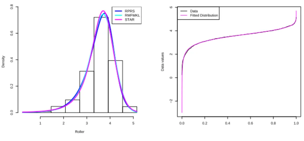
We also apply the resample Kolmogorov-Smirnov test[Su 17]for the goodness-of-fit pur-pose. There are 960 times out of 1000 times that the p-value does not reject the null hypoth-esis, which indicates the sufficiency of the GLD fitting. Left graph in Figure 1 shows the fitted GLD density function with the histogram of the roller data. Three different estimated GLD density functions with different colors provided by GLDEX package [Su 17]. The dark blue one with the label RPRS corresponds to the GLD introduced in Section 2 due to Ramberg and Schmeiser[13], which is estimated by the maximum likelihood method. The light blue one with the label RMFMKL corresponds to a slight different version of GLD due to Freimeret al.
[3], which is estimated by the maximum likelihood method. The pink one with the label STAR corresponds to the Freimeret al. [3]version of the GLD, which is estimated by the starship method [King and MacGillivray 6]). The right graph in Figure 1 is the quantile plot of the Ramberg and Schmeiser[13]version of the GLD fits. In Table 1, the estimated values of GLDs are all for Ramberg and Schmeiser[13]version of the GLD. From the graphs and tables, we can see the GLD fits the data pretty well. In Table 1, we also compare the first four moments of the real data with those of the fitted GLD distribution. From comparison we can observe that the moments of the fitted GLD are close to true moments of the data.
Roller
Density
1 2 3 4 5
0.0
0.2
0.4
0.6
0.8
RPRS RMFMKL STAR
(a) Histogram of 1150 roller with GLD fits.
0.0 0.2 0.4 0.6 0.8 1.0
−2
0
2
4
6
Data values
Data Fitted Distribution
(b) Quantile plot for GLD fits of the data using maximum likelihood estimation.
Table 1: Moments comparison of roller data and the fitted GLD.
DATA GLD
Mean 3.53474 3.53544
Variance 0.42212 0.42135 Skewness −0.98659 −0.98786
Kurtosis 4.86310 5.53253
4.2. Pollen Data
The second data is pollen data which also is available from Carnegie Mellon University†. We fit the variable “nub”, which consists of 481 values from measuring geometric charac-teristics of certain type of pollen with a GLD model. We obtain the estimated parameters of an assumed GLD distribution of the data as λˆ1 = −0.425, λˆ2 = 0.240 and λˆ3 = 0.328,
ˆ
λ4 =0.186 with the R package GLDEX. Following the procedure proposed in Section 3, we
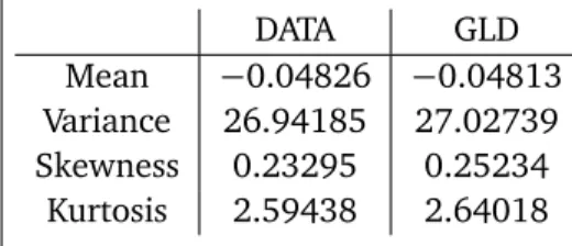
generate 1000 samples withG L D(−0.425, 0.240, 0.328, 0.186)with the sample sizen=481. The test statistic is calculated from (12) with the approximated p-value as 0.156, which leads to fail to reject the null hypothesis at the significance levelα=0.05, that is, the data can be fitted by a GLD model sufficiently. The results are listed in Table 2 provides the comparison of the moments of the data and the fitted GLD. We observe that the moments of the GLD model are close to true values of the moments of the data.
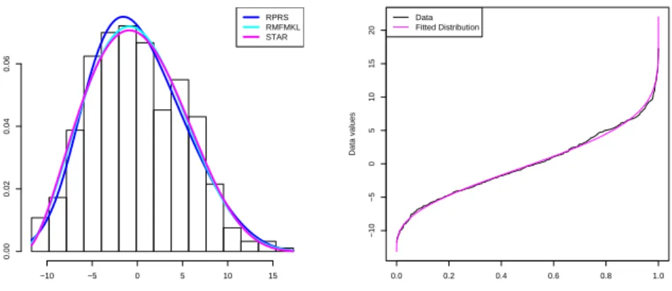
The resample Kolmogorov-Smirnov test[Su 18]shows that 959 times among 1000 times the p-value does not reject the null hypothesis, which indicates the sufficiency of the GLD fits. The histogram and quantile plots listed below also show the good fit of the GLD on the data. The left graph in Figure 2 shows the estimated density function of the GLDs by the maximum likelihood method and the starship method with the histogram of the pollen data. The colors have the same meaning as in the Figure 1. The right graph shows the quantile plot of the estimated Ramberg and Schmeiser[13]version of the GLD. We observe that the GLD fits the data very well.
Table 2: Moments comparison of pollen data and the fitted GLD
DATA GLD
Mean −0.04826 −0.04813 Variance 26.94185 27.02739 Skewness 0.23295 0.25234
Kurtosis 2.59438 2.64018
nub
Density
−10 −5 0 5 10 15
0.00
0.02
0.04
0.06
RPRS RMFMKL STAR
(a) Histogram of 481 observations with GLD fits.
0.0 0.2 0.4 0.6 0.8 1.0
−10
−5
0
5
10
15
20
Data values
Data Fitted Distribution
(b) Quantile plot for GLD fits of the data using maximum likelihood estimation.
Figure 2: Results of fitting GLD to the pollen data.
5. Discussion
In this paper, we investigate the problems of the goodness-of-fit for the generalized lambda distribution (GLD) family due to its high flexibility in the data fitting, especially for the heavy-tailed data. We propose an empirical likelihood based goodness-of-fit test for this distribution family. The motivation of the proposed test is based on the UMP likelihood ratio test guar-anteed by Neyman-Pearson lemma with the null and alternative distributions both known. However, in practice, the alternative distribution is usually not known. Therefore, the pro-posed nonparametric goodness of fit test is constructed to approximate the optimal test for the scenario with an unknown alternative distribution. Asymptotic results have been derived for the proposed test. Since the explicit form of the asymptotic null distribution is not avail-able and the test statistic is data dependent, we propose an empirical procedure through the simulations to approximate p-value of the test statistic for given data sets. The results show that the generalized lambda distribution offers sufficient fittings for both roller and pollen data sets, which match the conclusions obtained from the other goodness of fit tests such as the resample Kolmogorov-Smirnov test.
ACKNOWLEDGEMENTS The author would like to thank Professor Arjun Gupta for his valu-able discussions and suggestions.
References
[2] B. Fournier, N. Rupin, M. Bigerelle, D. Najjar, A. Iost and R. Wilcox. Estimating the pa-rameters of a generalized lambda distribution.Computational Statistics & Data Analysis, 51:2813-2835, 2007.
[3] M. Freimer, G. Mudholkar, G. Kolloa. and C. Lin. A study of the generalized Tukey lambda family.Communications in Statistics–Theory and Methods, 17:3547-3567, 1988.
[4] Z.A. Karian and E.J. Dudewicz.Fitting Statistical Distribution: The Generalized Lambda Distribution and Generalized Bootstrap Methods, Boca Raton, FL:CRC Press, 2000.
[5] Z.A. Karian and E.J. Dudewicz.Handbooks of Fitting Statistical Distributions with R. New York: CRC Press, 2011.
[6] R. King and H. MacGillivray. A starship estimation methods for the generalized lambda distributions.Australia & New Zealand Journal of Statistics, 41:353-374, 1999.
[7] A. Lakhany and H. Massuer. Estimating the parameters of the generalized lambda dis-tribution.Algo Research Quarterly, 47-58, 2000.
[8] W. Ning, Y.C. Gao and E.J. Dudewicz. Fitting Mixture Distributions Using Generalized Lambda Distributions and Comparisons with Normal Mixtures. American Journal of Mathematical and Management Science. Vol. 28, NOS. 1&2, 81-99, 2008.
[9] W. Ning and A.K. Gupta. Change point analysis for generalized lambda distributions.
Communication in Statistics-Simulations and Computation. 38:1789-1802, 2009.
[10] A.B. Owen. Empirical likelihood ratio confidence intervals for a single functional.
Biometrika, 75:237-249, 1988.
[11] A.B. Owen. Empirical likelihood ratio confidence regions.The Annals of Statistics, 18:90-120, 1990.
[12] A.B. Owen.Empirical Likelihood. New York: CRC Press, 2001.
[13] J.S. Ramberg and B.W. Schmeiser. An approximation method for generating symmetric random variables.Communications of the ACM, 15: 987-990, 1972.
[14] J.S. Ramberg and B.W. Schmeiser. An approximation method for generating symmetric random variables.Communications of the ACM, 17:78-82, 1974.
[15] J.S. Ramberg, P.R. Tadikamalla, E.J. Dudewicz and E.F. Mykytka. A probability distribu-tion and its uses in fitting data.Technometrics, 21:201-214, 1979.
[16] S. Su. A discretized approach to flexibility fit generalized lambda distributions to data.
Journal of Modern Applied Statistical Methods, 4:402-424, 2005.
[18] S. Su. Fitting single and mixture of generalized lambda distribution to data via dicretized and maximum likelihood methods: GLDEX in R.Journal of Statistical Software, 21:1-17, 2007.
[19] S. Su, A. Hasan. and W. Ning. (2013). The RS generalized lambda distribution based calibration model.International Journal of Statistics and Probability. 2:101-107, 2013.
[20] J.W. Tukey. The practice relationship between the common transformations of percent-ages of counts and of amounts. Technical Report 36, Statistical Techniques Research Group, Princeton University, 1960.
[21] O. Vasicek. A test for normality based on sample entropy. Journal of Royal Statistical Society, B, 38:54-59, 1976.
[22] A. Vexler and G. Gurevich. Empirical likelihood ratios applied to goodness-of-fit tests based on sample entropy.Computational Statistics and Data Analysis, 54:531-545, 2010.
Appendix
Proof. [Theorem 1]We consider the following statistic,
Tn=1
nlog1≤minm<n1/3 n
Y
j=1
2m
n(X(j+m)−X(j−m))
=− max
1≤m<n1/3tmn
where tmn = 1n
Pn i=1log(
n
2m(X(j+m)−X(j−m)). It is a part of n
−1log(G L D
n), where G L Dn is the test statistic defined in (12). Similar to the work by Vasicek[21], we rewrite
tmn=−1
n
n
X
i=1
logf(xi) +Vmn+Umn, (A1)
where
Vmn=− 1
n
n
X
i=1
log
F(x(i+m))−F(x(i−m))
f(x(i))(x(i+m)−x(i−m))
,
Umn= 1
n
n
X
i=1
log
n
2m(F(X(i+m))−F(X(i−m)))
.
where F is the distribution function of X0s. Denote Fn the empirical distribution function of
X0sand combine the first two terms in (A-1), we obtain
−1
n
n
X
i=1
logf(xi) +Vmn=− 1
n
n
X
i=1
logf(xi)− 1
n
n
X
i=1
log
F(x(i+m))−F(x(i−m))
f(x(i))(x(i+m)−x(i−m))
=−1
n
n
X
i=1
logf(x(i))−1
n
n
X
i=1
log
F(x(i+m))−F(x(i−m))
f(x(i))(x(i+m)−x(i−m))
=−1
n
n
X
i=1
log
F(x(i+m))−F(x(i−m))
(x(i+m)−x(i−m))
=− 1 2m
2m
X
j=1
n
X
i=1
log
F(x(i+m))−F(x(i−m))
(x(i+m)−x(i−m))
(Fn(x(i+m))−Fn(x(i−m))),
wherei≡ j (mod 2m). Let
Sj=− n
X
i=1
log
F(x(i+m))−F(x(i−m))
(x(i+m)−x(i−m))
(Fn(x(i+m))−Fn(x(i−m))),i≡ j (mod 2m),
then
tmn= 1 2m
2m
X
j=1
With the argument in Theorem 1. by Vasicek[21],
1 2m
2m
X
j=1
Sj→H(f), a.s,
as m/n→0 uniformly for all 1≤ m≤ n1/3, where H(f) =E(−logf(xi)) =E(−logf(x1). Since the statisticsUmn is a non-positive variable by the definition and is independent of F,
Umn→0 in probability asm→ ∞andn→ ∞by Lemma 1 in Vasicek[21]. Therefore,
Tn≤ −tn1/3,n p
→Ef(log(X1)),
Tn≥ − max
1≤m<n1/3(2m) −1
2m
X
j=1
Sj→p Ef(log(X1))
asn→ ∞. It implies that
Tn→Ef(log(f(X1))), asn→ ∞. (A2)
Now, we rewrite the test statisticG L Dnas
1
nlog(G L Dn) =Tn−
1
n
n
X
i=1
log(fH
0(Xi|λ))
+1
n
n
X
i=1
log(fH
0(Xi|λ))− n
X
i=1
log(fH
0(Xi|λˆn))
!
,
(A3)
whereλˆn= (ˆλ1,λˆ2,λˆ3,λˆ4). Under the null hypothesis,Tn→EfH0(log(fH0(X1)))in probability since (A2). With the condition(C1), we have
1
n
n
X
i=1
log(fH0(Xi|λ))→p EfH
0(log(fH0(X1|λ))). (A4)
With the condition(C2)holds and applying one-term Taylor Series expansion to the third part in the equation (A3), we obtain
1 n n X
i=1
log(fH
0(Xi|λ))− n
X
i=1
log(fH
0(Xi|λˆn))
∼= 1
n
n
X
i=1 4
X
j=1
hi(Xi;λnˆ )(θj−λˆn j),
wherehi(·)is defined in Section 2.3. Since(C4), we obtain
1
n{
n
X
i=1
log(fH0(Xi|λ))− n
X
i=1
log(fH0(Xi|λˆn))} ∼= 1
n
n
X
i=1 4
X
j=1
hi(Xi;λnˆ )(λj−λˆn j)
≥ 1
n
n
X
i=1 4
X
j=1
|hi(Xi;ξi)|(λj−λˆn j) p →0
where|ξi−λ| ≤ |λ−λˆn|. Thus under the null hypothesis, the equations (A3), (A4) and (A5) provide
1
nlog(G L Dn)
p
→0, asn→ ∞. (A6)
This completes the proof of Theorem 1.
Proof. [Theorem 2]UnderH1, we have 1
nlog(G L Dn) =Tn−
1
n
n
X
i=1
log(fH1(Xi)) +1
n
n
X
i=1
log
fH1(Xi)
fH0(Xi|λ0)
+1
n
n
X
i=1
log fH0(Xi|λ0)
fH
0(Xi|λˆn)
! (A7)
Since (A2), similarly underH1
Tn→EfH1(log(fH1(X1))), asn→ ∞, (A8)
and the condition (C1) leads to
1
n
n
X
i=1
log(fH1(Xi|λ))→p EfH
1(log(fH1(X1|λ))). (A9)
With the condition (C3),
1
n
n
X
i=1
log fH0(Xi|λ0)
fH
0(Xi|λˆn)
!
P
−→0 (A10)
asn→0. With the equations (A8),(A9) and (A10), we obtain,
1
nlog(G L Dn)
P −→1
n
n
X
i=1
log
fH
1(Xi)
fH0(Xi|λ0)