The Asian Journal of Technology Management Vol. 4 No. 1 (2011) 56-64
Interbank Lending Decisions in An Economic Downturn: An
Agent-Based Approach
Deddy P. Koesrindartoto*F
1
F
1, Erdi Novanto1
School of Business and Management, Institut Teknologi Bandung
ABSTRACT
Interbank lending is one mechanism that can make shock, which is accepted by one bank spread to other banks (contagion). There are several researchers that focused their research on analyzing the effect of interbank lending to systemic risk. However, there is a few research that analyzed the effect of banks’ decision maker’s behavior, especially on the bank interbank lending to the systemic risk. In this research, the author creates an agent-based simulation of the banking system to analyze the effect of banks’ decision maker’s behavior to systemic risk in economic downturn condition. The preliminary result from this research is for an economic downturn in a long time period, the banking system with a low net worth to the asset's ratio threshold will produce more default bank than the banking system with a high net worth to the asset's ratio threshold. However, for an economic downturn in small time period, banking system which all bank in their system has the higher net worth to assets ratio threshold will have the default bank first than the banking system which has the lower net worth to the asset's ratio threshold.
Keywords: agent-based simulation, banker behavior, interbank lending, economic downturn
*
1. Introduction
Systemic failure in the financial sector is one of the risk that many countries try to prevent. This caused by cost systemic failure has estimated to be large (Hoggarth et al., 2002) and crisis in all or part of banking sector can create cost on the economy of a country as a whole or parts within it (Hoggarth et al., 2002), (Kaufman, 1996).
There are several channels that can make shock accepted by one bank transmitted and to other banks (Upper, 2011). One of the channels is interbank lending. To study the effect of interbank lending and bank structure resilience to systemic failure, many researcher use computer simulation. However, there are few researches in this field that included the behavior of banks’ decision makers.
2. Literature Review
Systemic failure happened because loss (shock) that accepted by one bank transmitted to other banks. This property called bank contagion. Contagion in the banking system can take place through a multitude of channels (Upper, 2011). One of the channels of bank contagion is through interbank lending. In interbank market one bank can give lending to other banks that needs money. There are two functions that interbank market can do (Bhattacharya and Gale, 1987). The first function is as a device for co-insurance against liquidity shocks. The second function is as a mechanism to absorb shock that hit the banking system. However, interbank market also can give bad impact to the financial system. This is because interbank connection can make shock that accepted by one bank spread to other banks (contagion).
In order to study how interbank connection many researcher use computer simulation that based on graph theory. This approach used because the scarcity of theoretical results. Several researcher that use
this approach are Allen and Gale (1998), Allen and Gale (2000), Diamond and Dybvig (1983), and Rochet and Tirole (1996).
Nier et al. (2008) also used computer simulation to study about interbank connection. In their study they found that there are several aspects in bank system structure that can affect bank system resilience to systemic risk. Nier et al. (2008) shows how condition of bank’s net worth (capital), level of interbank lending, and level of capital can affect bank system resilience. One of their results is negative and non-linear relationship between contagion and capital. This result means higher capital can make the bank system more resilience to systemic risk. Although there are many research about systemic risk and interbank contagion, but there still the weakness on it. Based on Upper (2011) one of the weaknesses is there is no behavioral foundation in it. In reality, bank can anticipate the shock that can happen and make some preparation to face it. One of the anticipation that they can do is by taking back their lending from the bank that can go default.
In this paper, we analyze the effect of bank decision maker behavior and bank system structure, especially in their initial percentage of net worth.
3.1. Model Building
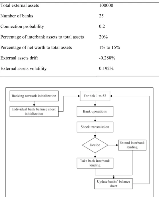
The general overview of the simulation process is described in figure 1. (See appendix figure1)
3.2. Bank Network Initialization
In this simulation, bank system represented as nodes and directed lines. Node represents a bank and directed line represented direct lending relationship from a bank that gives lending to bank that borrow money from that bank. To initialize the bank network, we use two parameters, that is the number of bank (N) and connection probability, that is, probability one bank has lent to another bank (p). We make simplification by use same connection probability for each bank.
3.3. Model of Individual Bank Balance Sheet
After banking network already constructed, we develop individual bank balance sheet. In agent-based simulation, bank represented as the agent and bank balance sheet represented as agent properties. The to develop individual balance sheet, we use same approach developed by Nier et al. (2008). In their approach, they begin from general banking system properties such as initial total external asset, initial number of bank, connection probability, percent interbank to total asset, percent net worth to total asset. From these properties, they applied some algorithm and made every bank have their individual balance sheet. Bank individual balance sheet consist of external assets and interbank assets in their asset's side and their liabilities side consists of customer deposit, interbank borrowing, and net worth.
4. Model of Banks Operation
To simulate how bank decision maker behavior react to changing in their environment, we create this simulation in multi-period simulation. In the multi-period simulation how assets and liabilities changes dynamically over time should be modeled. Assets of a bank will change every time depends on profit or loss that they get from their assets’ allocation. Their liabilities will also change because a bank must give interest to their depositor, and their net worth will change depends on the value of the assets and depositor’s deposit or interbank borrowing.
In this study, assets of a bank are divided into two parts, there are the external assets, denoted by v, and interbank asset, denoted by d. External assets in this study change dynamically following the geometric Brownian motion with constant drift μ and volatility σ > 0 where W is standard Brownian motion. This approach is also used in Liang et al. (2011) in their paper to create a model of a bank running for liquidity risk. For time t ∈ (0, T), value of external assets follows (2), value of interbank assets or bank lending with interbank lending intere rst ate ri follows (3).
(3) (2)
Liabilities sides of the bank are divided into three parts, there is the customer deposit, denoted by d, interbank borrowing, denoted by
b, and net worth, denoted by w. For time t ∈
5. Shock and Shock Transmission
In this study, shock defined as all circumstances that can reduce the value of a bank’s external assets or interbank asset. Value of a bank’s external assets can be reduced because of loss or depreciation in their investment or credit default. Reduce in interbank asset happened because other banks that borrow money from this bank default and can’t give back all money that they borrow.
In general, if a bank gets a small shock this bank only loses a small amount of money, and they will withstand the shock. However, if the shock is bigger than the bank's net worth then this bank default. If the net worth can’t absorb all shock, the residual transmitted to creditor banks through interbank liabilities. This shock will transmit equally to every bank that gives lending to bank that get that shock. If interbank liabilities still cannot absorb the shock, then shock is absorbed by depositors.
In this study, if one bank is default, then this bank takes all his lending and gives back this bank’s borrowing to bank that gives this bank lending. Banks that give lending to the default bank put money, that default bank gives back, to its external asset. Bank that borrows from this bank must give back their borrowing and balance their balance sheet by reduce their external asset.
6. Bank’s Decision on Their Interbank Lending
In each tick, every bank will analyze other banks financial condition. We simplified how each bank sees other banks financial condition by their net worth to the asset’s ratio. Bank with a low ratio indicates their financial strength is not in good condition. Bank with a high ratio indicates their financial strength in good condition and can accept bigger shock.
In this simulation, every bank has the same threshold which if other banks that they
give lending have the net worth to the asset's ratio threshold lower than this threshold, then the bank that gives lending will take back their lending. In this simulation, by using the different net worth to the asset’s threshold we analyze how bank behavior in manage their interbank lending can make the difference in bank system resilience.
7. Simulation Result
To see how the initial percentage of net worth and behavior of the bank decision makers in their interbank lending, we simulate the model that already developed with parameter that shown in table 1. (See appendix table 1)
To mimic economic downturn, we use negative external assets drift. Each simulation consists of 52 ticks. In each tick, each bank external assets decrease follows geometric Brownian motion with negative drift. In this simulation, we assume that in the economic downturn every bank not makes new lending to other banks. They only take decisions do they take their lending from other banks or not.
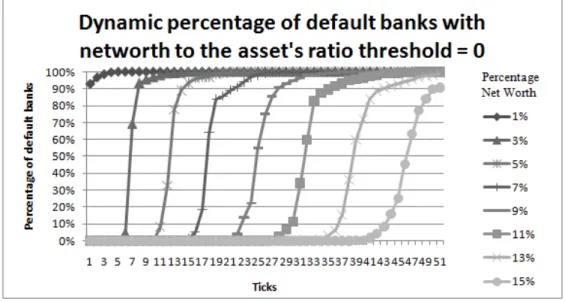
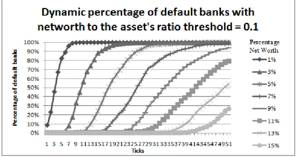
In this study, we use six net worth to the asset's ratio threshold from 0%, 2%, 4%, 6%, and 8%. Bank with the net worth to the asset's ratio threshold equals to 0% represented as the bank that their decision maker still not takes their lending even bank that borrows to them nearly default. These different thresholds represent the different behavior of the bank decision makers in the bank system. We simulate this simulation 50 times and get the average results and present the simulation results in figure 3, 4 and 5. (See appendix figure 3,4,5)
For a long-term economic downturn, we can conclude that behavior of the bank decision makers have an impact to number of the bank that defaults. In this simulation, bank system with behavior of their agent who take back their lending when their borrower net worth to the asset's ratio reaches the lower threshold have more percentage of default banks higher than the bank system with behavior of their agent who takes back their lending when their borrower net worth to the asset's ratio threshold higher.
In the small time period, we can conclude that bank system with the higher percentage of net worth can survive in the economic downturn in the small time period than the bank system with the lower percentage of net worth. Behavior of bank decision makers in extending or take back their loan effect to number of default banks. In the bank system with the same percentage of net worth, the higher net worth to the asset's ratio threshold that their agent has the increase of the number of default banks will be slower than the bank system with the lower net worth to the asset's ratio threshold that their agent has. This result happened because the bank system with behavior of their member has the higher net worth to the asset's ratio threshold have fewer probabilities to get the shock that transmitted from interbank market.
8. Conclusion
This study shows how the percentage of net worth before the bank system at the beginning of an economic downturn and how behavior of the bank's decision makers in extending their interbank lending can affect bank system resilience to systemic failure.
In general, for all percentage of net worth, banking systems with behavior of their bank that take back their lending when their borrower percentage of net worth higher has the lower number of default banks than banking systems with behavior of their bank
that take back their lending when their borrower percentage of net worth lower. However, banking system with behavior of their bank that take back their lending when their borrower percentage of net worth higher has the defaults bank in advance rather than banking systems with behavior of their bank that take back their lending when their borrower percentage of net worth lower.
From that result, the central banks or financial regulators should pay attention and monitor percentage of net worth (capital) and interbank lending, especially when a country face both in short or long time durations of an economic downturn. With appropriate policies to regulate the behavior of the bank, then the number of bank that defaults can be reduced.
References
Allen, F., & Gale, D. (2000). Financial Contagion. Journal of Political Economy , 108(1), 1.
Allen, F., & Gale, D. (1998). Optimal Financial Crises. Journal of Finance , 53(4), 1245-1284.
Axtell, R. (2000). Why agents? on the varied motivations for agent computing in social science. Working paper 17, center on Social and Economics Dynamic .
Bhattacharya, S., & Gale, D. (1987). Preference Shocks, Liquidity, and Central Bank Policy. Proceedings of the Second International Symposium in Economic Theory and Econometrics (pp. 69-88). New York and Melbourne: Cambridge University Press.
Diamond, D., & Dybvig, P. (1983). Bank Runs, Deposit Insurance, and Liquidity. Journal of Political Economy , 91(3), 401-419.
Empirical Evidence. Journal of Banking & Finance , 26(5), 825.
Kaufman, G. (1996). Bank Failures, Systemic Risk, and Bank Regulation. CATO Journal , 16(1), 17.
Liang, G., Lütkebohmert, E., & Xiao, Y. (2011). A Multi-Period Bank Run Model for Liquidity Risk. Working paper from the Oxford-Man Institute .
Nier, E., Yang, J., Yorulmazer, T., & Alentorn, A. (2008). Network Models and Financial Stability. Bank of England. Quarterly Bulletin , 48(2), 184.
Novanto, E. K. (2011). The Effects of Bankers' Strategy on Systemic Risk in Banking Industry: An Agent Based Approach. Industrial Engineering and Service Science 2011. Solo.
Rochet, J., & Tirole, J. (1996). Interbank Lending and Systemic Risk. Journal of Money, Credit & Banking , 28(4), 733-762.
Appendix
Table 1. Summary of benchmark parameter
Parameter Simulation Benchmark
Total external assets 100000
Number of banks 25
Connection probability 0.2
Percentage of interbank assets to total assets 20%
Percentage of net worth to total assets 1% to 15%
External assets drift -0.288%
External assets volatility 0.192%
Figure 2. Example bank network consists of twelve banks