Vol 62, No 1 (2019)

TECHNICAL UNIVERSITY OF CLUJ-NAPOCA

ACTA TECHNICA NAPOCENSIS

Series: Applied Mathematics, Mechanics, and Engineering Vol. 62, Issue 1, March, 2019

A THEORETICAL APPROACH ON DETERMINING THE GEOMETRICAL

ERRORS IN CASE OF ARTICULATED ROBOT STRUCTURES

Ovidiu-Aurelian DETEȘAN, Adina Veronica CRIȘAN

Abstract: The purpose of this paper is to bring in a mathematical model for determining the matrices of geometrical errors. To this effect, the matrices of input data were presented as well as a model of computing the primary errors from the driving joints, the obtained results being essential in defining the geometric errors that affect the work performances of the articulated robot structures. The assessment of robot performances can be achieved by considering the xth order differential model of errors. The linear model of position and orientation errors and the cumulative errors corresponding to transformations between robot systems are also determined.

Key words: articulated robot, geometric errors, accuracy, geometry, differential operator. 1. INTRODUCTION

Robot manipulators are essential components of any robotic manufacturing system, being used in most of the industrial applications. Both, design and the implementation of robots are based on the modeling, analysis as well as the accurate programming of the characteristic point in the work space. In different applications such as welding, handling or inspection of parts, it has been noticed that the accurate positioning of the robot's characteristic point was a very difficult task for the robot.

The factors that influences the positioning accuracy of the characteristic point in the work space are the variations of the geometric parameters from the robot joints, of which the dimensions of the kinetic elements and the joint orientation, are considered main sources of the position errors. The reason is that the kinematic modeling is achieved by considering the geometric parameters to determine the position of the characteristic point, as well as the generalized coordinates of each joint.

The main function of a robot is to handle different objects, materials or tools at any point in the workspace and it can perform various tasks, at a certain level of accuracy. In operating the articulated robot structures, the position and orientation of the end effector are influenced by

2. THE INPUT DATA

2.1 The matrices of the input data

The first step in the modeling of the kinematic accuracy of robots, according to [16] consists in computing the matrices of the input data, also known as the matrices of robot geometry.

So, considering a robot mechanical structure characterized by n degrees of freedom, for each element belonging to the nominal (errorless) and to the real (affected by errors) robot mechanical structure are established the following: the coordinates of the geometric center of each driving joint, denoted with O_i as well as the position of a certain point A_i, randomly chosen on the kinematic axis k_i, both of them being referenced to the fixed system attached to the robot base  0 .

To establish the matrices of input data the following notations are considered: n which is the number of driving joints (d.o.f), m represents the number of robot distinct configurations, q

 

n r, where n represents the nominal values and r the real values of generalized coordinates or robot links.

The matrices of the input data are established by following some steps. The first one consists in establishing the geometric model of the considered robot structure for a certain configuration. In this respect, the nominal values of the points O_i are given, with respect to 0 , according to specifications.

The collected data is entered in a n 1 6  matrix called the matrix of nominal geometry and denoted with M_vnand defined as follows:

 0

, 1 1

 

_ nT nT_T   

vn i i

M p k i n ; (1)

where p_inT represents the nominal position of the geometric center of each driving joint and

nT i

k defines the orientation of each driving axis also in the nominal configuration (errorless). The components of the real geometry matrix

 0 vr

M are determined by physical measurements:

 

 





0

1 6

, 1 1

     

 

 _ rT rT_    T

vr i i

n

M Matrix p k i n _{; (2)}

where p_ir T represents the real position of the geometric center of each driving joint and k_ir T defines the orientation of each driving axis, in the real configuration (with errors). The orientation of systems attached in the geometrical center of each robot joint is established next. All the systems will have the same orientation with the fixed system  0

attached to the robot base. For qn and 1

 

i n the length of kinetic element

 

iq is determined, according to:



 

 



1

2 2 2

1 1 1



  

 _{  } 

 

 

      

 

q q q

i i i

q q q q q q

i i i i i i

L p p

x x y y z z

; (3)

The orientation of each driving joint

 

iq is established using the following expression:





, , ,

  

 

_{ }T 

qT q q q

i iu iu iu

k c c c u x y z ; (4)

Next, the n 2 9 matrix of nominal systems denoted with T_n 0 is written:

 0

, 1 1

 

_ nT nT nT nT_T   

n i i i i

T p x y z i n ; (5)

Based on (3) and (4) the n 1 6 matrix of robot nominal geometry



M_Gn



is established:

, 1 1

  

 

_ n n n n n n_T   

G n i i i i i i

M x y z i n ; (6)

For qr and i n 1 the elements of the

 0 vr

M matrix are used, previously defined with (2).

In the real configuration the n 2 9 matrix of real systems is defined, denoted with T_r 0 , as:

 0

, 1 1

 

_ rT rT rT rT_T   

r i i i i

T p x y z i n ; (7)

as: _    _ ,   1 1

T

r r r r r r

G r i i i i i i

M x y z i n ;

(8)

For i 1 n, the next step consists in computing the homogenous transformations between the  i and i 1 mobile frames.

The general expression for defining the homogenous transformations is the following:

 



   



1

1 1

1

1 1 1 _{0 0}

10 1

0 0 0 1

0 0 0 1



 



  

 

   

 _ _ 

   

 _ _ 

 

 _{ }

 _{   }

_{  }

 _{ }

  

 

n i n i i i i n

i i

T

i n i n i n n n n

i i i i i i

R p

T

x y z _{R p p}

; (9)

where T_{i i}n_1 represents the nominal value of the homogenous transformation between the  i and i 1  frames, R_{i i}n_1 is a 3 3  matrix which defines the orientation of each driving axis of the mobile frame  n with respect to the fixed frame  0 attached to robot base, in the nominal configuration and i1p_{i i}n_1 is a 3 1 

column vector expressing the position of each frame  i with respect to the previous frame

 i1 for the same nominal configuration. Similarly, for i 1 n and qr are computed the homogenous transformations between  i and i 1  frames, where T_{i i}r_1 and its components have the same meaning as in (9) the only difference being that this time the real robot configuration is considered.

By the similarity with the properties of the time derivative of the locating matrix, according to [3] – [12], the following relation between the homogeneous transformation for robot nominal structure and the real transformation matrix

1 r i i

T _ results:

1 1 1  1 1 1

           

r n n n

ii ii ii ii ii ii

T T T T T T ; (10)

1 1  1

  

  n 

ii ii ii

T T T ; (11) where T_ii1 is the first order differential error of the homogenous transformations between

 i and i 1  reference frames.

In order to determine the expression for the matrix operator of errors, the following equation is used:

1  1 1 1

      

n r n

ii ii ii ii

T T T T ; (12) The equation is multiplied left side by

 

T_iin_1 1. Applying the matrix properties, it results finally:

 

 

 

1

1 1 1

1 1

1 1 1 1





  

 

   

 _{  } 

 

 

_{   } 

 

n n

ii ii ii

n r n n

ii ii ii ii

T T T

T T T T

; (13)

where,

 

T_iin_1 1T_iin_1I₄. (14) The final expression for the matrix operator of errors is obtained in the following form:

 

1

1 1 1 4

Tii  Tiin  Tiir  I . (15)

where T_iin_1 and T_iir_1 were previously defined according to (9) and

 

T_iin_1 1is the inverse matrix of the T_iin_1 homogenous transformation. It is a fact that the position and orientation errors are mainly caused by deviations of the relative positions of the driving joints, by the plays in driving joints, the deformations of the kinetic links or by the oscillation of the mechanical, driving or control system. So, for

1  

i n the matrices of primary errors are established, which are in fact the relative errors from the robot driving joints:





1

1

0 0 0 1



 _      

 

 

i ii

ii

p

T ; (16)

where



 _i



is a antisymmetric matrix that includes the relative errors for orientation

 

 ,  and  , p_{ii 1} representing the column vector of relative errors for positioning:

1 1 1

  

  r  n

ii ii ii

measurements). The validation tests allow to determine the value of an experiment based on the probability of occurrence of a variation in the work environment. By performing these tests, it can be determined whether a certain experimental result is not an aberrant result caused by external factors.

Also it can determine if the same result can be considered within the limits of normal variability and does not negatively influence the conduct of the experiment.

Next, the T_{ii 1} matrix operator is established by considering the following notations:

 

;

yQ yS

   y



p_Q; e; g



; (18)



; ; ;  ; ;



 

Q S xi yi zi i i i

p p p p p ; (19)

where y represents an index which highlights the locating errors (position and orientation errors) corresponding to: p_Q - each parameter, e - each element and g - to the whole robot mechanical structure.

The n 1 6 matrix of locating errors, symbolized with E_spk is established, n representing the number of elements which make up the mechanical structure of the robot. For the nominal and real structure, the n6 matrix of nominal/real configurations of the robot is determined, M_q



qn r,



defined as following:

M_q=__kqT, k 1 m_; (20)

where _kqT _q_ikq, i 1 n_. (21)

Table 1 n

M_

ij n

M_

Joint type

Nominal values

Mechanical restrictions

R_, T q_in qn_i q_in q_inmax q_inmed q_inmin

Table 2 r

M_

ij n

M_

Real values

Errors



, , 



Mechanical restrictions r

i

q qr_i qr_i q_i q_i q_i qmax_ir qmed_ir qmin_ir

In Table 1 and Table 2 the components of the matrix of nominal / real configurations of the robot are represented.

The time matrix is determined according to:



, 1



  

t i

M t i m ; (22) where t_m...[s] represents the time required to achieve the m configuration.

The matrix of real robot configurations is determined by performing physical measurements on the real structure.

3. MODELING OF GEOMETRICAL ERRORS

3.1 Determining of primary errors

This section aims to determine the primary errors from the driving joints, due to plays, manufacturing errors or to the generalized coordinate’s errors, which are used for defining the geometric errors that affect the operation performances of the articulated robot structures.

The primary errors for two important sets of rotation angles – Bryant angles and Euler angles are determined further. For the set of Bryant angles



  _x _y _z



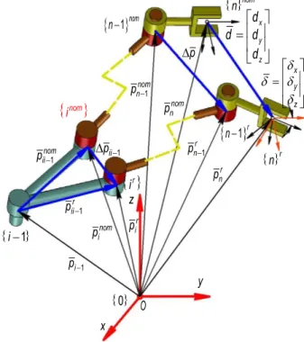
the primary errors are:

Fig. 1 The geometrical errors

z

O x  _i1

y

nom i

p pir

i

p_1

 _ir

 _inom

nom ii

p1

r ii

p_1

ii

p1



p 

x y z



 

     

   

 n1nom

 n1r

r n

p1 nom

n

p1

r n

p

nom n

p

 0

 nom

n

 r

n

x y z

d

d d

d

    

1 0

1 0 0 1 0

0 1 0 1 0 1 0

0 1 0 1 0 0 1

1 1 1                      _{  } _{ } _{  } _  _{ }           _{  }         _    _   _{  }      y _z x z x y z y z x y x

. (23)

The terms contained in (23) are identified with the terms contained in the following matrix:



 

 





 

 





 

 



1 1 1 1 1 1

1 1 1 1 1 1

1 1

1 1 1 1 1 1

                     _{  }       _    _  _{  }     

i nT i r i nT i r i nT i r

i i i i i i

nT r i nT i r i nT i r i nT i r ii ii i i i i i i

i nT i r i nT i r i nT i r

i i i i i i

x x x y x z R R y x y y y z z x z y z z

. (24)

By identification results the orientation errors:









1 1 1 1 1 1 ;              _{  }       

i nT i r

x i i

i nT i r

y i i

i nT i r

z i i

y z

x z

x y

(25)

For checking, the identities are written as:









1 1 1 1 1 1 ;               _{  }       

i nT i r

x i i

i nT i r

y i i

i nT i r

z i i

y z

x z

x y

(26)

The matrix operator of the primary errors for



  x y z



resultant rotation is defined as:





 

1

1

0 0 0 0

  _             ii ii p

T x y z ; (27)

 

 

_{ }

 

 

 

 

0 0 0                 _  _ _{ }    z y z x y x

; (28)

where 

 

_x  _y·s _z  _x·c _y·c _z; (29) 

 

_y  _y·c _z  _x·c _y·s _z; (30)

 

    · 

 _z  _z  _xs _y; (31)

1 1 1 1 1 ₁ 1 1 1 1 ·( · · · ) ·( · · · ) · · ·( · · · ) ·( · · · ) · · · · · ·                                  _                         

y_ii x z z x y z_ii x z x z y

x_ii y z y_ii x z x y z ii z_ii z x x y z

x_ii y z x_ii y z_ii x y

yii

p c s c s s

p s s c c s

p c c

p c c s s s

p p c s c s s

p c s

p s p c c

p c · 

                           

 y s x 

. (32)

For the set of Euler’s angles



_z _x _z



the angular errors are determined similar to the case presented in the previous example:

1 0 0

1 0 1 0

0 1

1 0 1 0

0 1

0 0 1 0 0 1

1 0 1 0 1                      _ _ _ __ _        _ _ _{ } _ _ _                _{   }          _      z z x z z x z z

z z x

x

.(33)

By identifying the terms from (33) with the corresponding terms from (24) are obtained:

1 1

  

  i nT i r

x zi yi ; (34)

1 1

   

    i nT i r

x z xi zi . (35)

If the condition_x 0 is satisfied, it results:





1 1

1 1 1 1 1                

i nT i r i nT i r i i

z i i _{i nT i r}

x i i

x z x z

z y ; (36)

1 1

   

   i nT i r

x z zi xi ; (37)





1 1

1 1 1 1 1                

i nT i r i nT i r i i

z i i _{i nT i r}

x i i

z x z x

z y . (38)

The analytical expression defining the differential operator relative to the primary errors contained in T_ii1



z x z 



, the equivalent with the Uicker operator, is determined as follows:





 

1

1

0 0 0 0

  _             ii ii p

The matrix of orientation errors is defined as:

 

 

 

 

 

 

 

0

0

0

 

  

 

   

 

 

    

 

_{ } 

 

z y

z x

y x

; (40)

 

  ·    · ·

 _x  _xc _z  _zs _xs _z; (41)

 

   ·  ·

 _y  _zs _xc _z  _xs _z; (42)

 

    · 

 _z  _z  _zc _x; (43)

1 1

1 1

1 ₁

1

1 1

1

·( · · · )

·( · · · )

· ·

·( · · · )

·( · · · )

· ·

· · ·

·

         

 

         

 

  









 _



 



  

  



  

    



   



x_ii z z x z z y_ii z z z x z

z_ii x z

y_ii z z z x z ii x_ii z z x z z

z_ii z x

z_ii x y_ii z x xii

p c c c s s

p c s c c s

p s s

p s s c c c

p p c s c c s

p c s

p c p c s

p s ·

 

 

 

 

 

 

 

 

 

 

 

 

 

 

 

 

 zs x 

. (44)

The expressions (32) and (44) represent the position errors from every driving joint which is a function of the orientation angles.

3.2 The matrices of geometrical errors

In this section are presented the matrices of geometrical errors according to [16], [3] - [12]. The first order differential error corresponding to homogenous transformation between  i and i1reference systems is determined using the following expression:

 1

1 1  1

  

  n 

ii ii ii

T T T ; (45) where T_{ii 1}n_ andT_{ii 1} are defined with (9) and (16). For i  1 n 1 and j 1 i the following first-order error differentiation matrix operators are determined:j1T_ii1, T_ij 1_1, T_ij1_1, T_ij1_1.

 1 1

1 1 1 1

   

      

j

ii ij ii ij

T T T T ; (46)

where j1T_ii1 represents the error differentiation matrix operator with respect to the errors from the driving joint  i , which include the local error differentiation operator. The T_ij1 along with its inverse is obtained as:





1 1

 

 



i

ij kk

k j

T T ; T_ij_1₁

 

T_ij1 T. (47)

The assessment of the robot performances is achieved by considering the xth order differential model of errors, wherex



1, 2, 3



. The differential model of errors is first applied on the homogenous transformation between the systems  0 and n . The first order differential matrix operator T_ij 1_1 is determined. It includes the cumulative error operator, as it results from:

 1  1

1 1

  

 

 



i j

ij kk

k j

T T . (48)

Thus, according to [5], [16], the matrix of geometrical errors which characterizes the linear model is defined by the expressions:

 



_{   } 1



0 1 0 1 0

1 1

   

 





n  i 

n i ii i

i

T T T T ; (49)

   



1



0 1 0 0 1 0

1 1 1 1

1 1

    

   

 





n 



n  i 

n ii i ii i

i i

T T T T T ;(50)

where 0 1T_n is the linear model of position and orientation errors, being defined as follows:

0 1

0 0 0 0

0 0

0

0 0 0 0

 

 

 

 

 _  _ 

 _ _ 

 

 

 



 

 

 

 _ 

  

 _ 

 

 

 

 _{ } 

 

n

x y z

d T

z y d

z x d

y x d

; (51)

where d  _d_x d_y d_z_T is the linear position error and   _  _{x y z}_T is the orientation error.

between  i and

 

j1 systems, are defined by means of the expression presented below:

1 1

ij 1 ij 1 ij 1

T_ T_ T_

   . (52)

In order to increase the positioning and orientation accuracy of a serial structure robot, it is recommended to compute the higher order differential errors, which are going to be presented in a future paper.

The equation (51) defines the forward model and can be applied in case that the primary geometric errors of the parameters which characterizes each element are known.

4. CONCLUSION

The main purpose of the industrial robots is to achieve the positions and orientations of the manipulated parts, which were previously prescribed, its accuracy being influenced by the values of the positional deviations, to which are added the deviations in displacements, speed, accelerations and forces respectively. In other words, the accuracy of any industrial robot can be evaluated by means of errors. The errors are defined as differential quantities which are represented by the difference between a nominal value that have to be achieved and that have been previously programmed and the reached value (actual or real value). The accuracy of industrial robots can be evaluated by means of two types of errors: systematic and random errors. The position and orientation errors are random errors while geometric (structural) errors falls into the category of systematic errors. The position error is a vector whose origin is represented by the coordinates of the point specified in the robot program and as application point the coordinates of the point that is reached in reality by the robot (the difference between the programed position and the achieved position). The orientation error is represented by means of an angle which has as its sides the programmed position and the achieved position of the characteristic straight line. The present paper aims to show a mathematical model for determining the matrices of geometrical errors. To this effect, first, the matrices of input data were presented. It was also presented a model of computing the primary

errors from the driving joints, the results being essential in defining the geometric errors that affect the working performances of the articulated robot structures. The assessment of robot performances can be achieved by considering the xth order differential model of errors, where



1, 2, 3





x . In this paper the linear model of position and orientation was determined, as well as the cumulative errors corresponding to the transformations between the systems. In order to increase the positioning and orientation accuracy of a serial robot structure, it is recommended to compute the higher order differential errors, which are going to be presented in a future paper.

5. REFERENCES

[1] Abderrahim, M., Khamis, A., Garrido, S., Accuracy and Calibration Issues of Industrial Manipulators, Industrial Robotics: Programming, Simulation and Applications, Low Kin Huat (Ed.), ISBN: 3-86611-286-6, Publisher Pro Literatur Verlag, Germany / ARS, Austria, 2006.

[2] Albers, A., Frietsch, M., Sander, C., Improving Positioning Accuracy of Robotic Systems by Using Environmental Support Constraints – A New Bionic Approach, Social Robotics , Lecture Notes in Computer Science Volume 6414, pp 192-201, Online ISBN 978-3-642-17248-9, 2010.

[3] Negrean, I., Contribuții la optimizarea parametrilor cinematici și dinamici în vederea măririi preciziei de funcționare a roboților, Teză de doctorat, Cluj-Napoca, Romania, 1995.

[4] Negrean, I., The Influence of Denavit-Hartenberg Type Parameters Upon Robot Kinematic Accuracy, The Second ECPD International Conference on Advanced Robotics, Intelligent Automation and Active Systems, Vienna, 1996, pp.474-479.

[6] Negrean, I., Vușcan, I., Modelling of Dynamic Accuracy for Robots, Second Part - The Model of Optimising Kinematic and Dynamic Accuracy, The Seventh IFToMM International Symposium on Linkages and Computer Aided Design Methods, Bucharest, August 1997, Vol.II, pg. 239-244.

[7] Negrean, I., Kinematics and Dynamics of Robots-Modelling-Experiment-Accuracy, Editura Didactică și Pedagogică R.A., ISBN 973-30-9313-0, Bucharest, 1999.

[8] Negrean, I., Negrean, D. C., The

Matrix-Differentiating Operators in Robot

Kinematics, Cluj-Napoca, Acta Technica Napocensis, Series: Applied Mathematics and Mechanics, 2001, Vol. 2, pg. 15-22.

[9] Negrean, I., Albețel, D.G., The Generalized Matrices in the Robot Accuracy, Conferința

Științifică Internațională TMCR 2003, Chișinău, 2003, Vol.3, ISBN 9975-9748-3-X. [10] Negrean, I., Negrean, D.C., New

Formulations about the Differential Matrices in Robotics, The first International Conference “Advanced Engineering in Mechanical Systems ADEMS’07” Published in the Acta Technica Napocensis, Series: Applied Mathematics and Mechanics, Vol. II, 2007, pg. 45-50, Cluj-Napoca, Romania. [11] Negrean, I., Duca, A.V, Negrean, D.C.,

Kacso, K., Mecanica avansată în robotică,

Editura UT Press, Cluj-Napoca, 2008, ISBN 978-973-662-420-9.

[12] Mircea, A., Kacso, K., Vușcan, I., Negrean, I., Morariu-Gligor, R., Determining the Errors Compensations by Using Numerical Simulation, Acta Technica Napocensis, Series: Applied Mathematics and Mechanics, Vol. 54, Issue IV, pg. 635 - 638, Cluj – Napoca, 2011.

[13] Negrean, I., New Aproaches on Notions from Advanced Mechanics, Acta Technica Napocensis, Series: Applied Mathematics and Mechanics, Vol. 61, Issue II, June, pg. 149 - 158, Cluj – Napoca, 2018.

[14] Renders, J.M, Rossignol, E., Kinematic Calibration and Geometrical Parameter Identification for Robots, IEEE Transactions on Robotics and Automation, Vol. VII, pg. 721 – 731, 1991.

[15] Ursu – Fischer, N., A Computing Method for the Positional Accuracy for the R-R-R

Type Serial Robot, Acta Technica

Napocensis, Series: Applied Mathematics and Mechanics, Vol. 59, Issue III, September, pg. 259 - 268, Cluj – Napoca, 2016.

[16] Duca, A.V., Cercetări și Contribuții privind Modelarea Preciziei Roboților cu Structură Serială, Teză de Doctorat, Cluj-Napoca, Romania, 2012.

O abordare teoretică privind determinarea erorilor geometrice in cazul structurilor articulate de roboți Scopul acestei lucrări este de a propune un model matematic pentru determinarea matricelor erorilor geometrice. În acest sens, au fost prezentate matricele datelor de intrare, precum și un model de calcul al erorilor primare care apar în cuplele motoare, rezultatele obținute fiind esențiale în definirea erorilor geometrice care afectează performanțele de lucru ale structurilor articulate de roboți. Evaluarea performanțelor unui robot se realizează luând în considerare modelul diferențial al erorilor având ordinul

x. Se determină, de asemenea, modelul liniar al erorilor de poziție și orientare și erorile cumulate de ordinul întâi corespunzătoare transformărilor omogene care au loc între sistemele atașate robotului.

Ovidiu-Aurelian DETEȘAN, Ph.D., Assoc. Prof., Eng., Technical University of Cluj-Napoca, Faculty of Machine Building, Department of Mechanical System Engineering, email: [email protected], phone: +40-64-401667, B-dul Muncii no.103-105, Cluj-Napoca, Romania.