CAS: The Optimal Number of Quantiles for Predictive Performance Testing of the NCCI Experience Rating Plan

(1)

for Predictive Performance Testing

of the NCCI Experience Rating Plan

by Jon Evans and Curtis Gary Dean

ABSTRACT

Quantile testing is a key technique for fitting parameters and

test-ing performance in workers compensation experience rattest-ing and

the number of quantile intervals must be specified for such a test.

A model is developed to compare the error in the quantile test

empirical estimates of relative pure loss ratios to the interquantile

differences between expected pure loss ratios. Theoretical model

predictions are compared to empirical results from bootstrap

quintile tests of the National Council on Compensation

Insur-ance (NCCI) Experience Rating Plan (ERP). The model predicts

that the noise-to-signal ratio grows in proportion to the 1.5 power

of the number of quantiles and in inverse proportion to the 0.5

power of the sample size of risks. Empirical quintile and decile

tests of NCCI’s Experience Rating Plan are consistent with model

predictions. Increasing the number of quantiles requires a much

greater proportional increase in data volume to maintain a

con-stant noise-to-signal ratio. This explains the use of few quantiles,

specifically quintiles, for testing NCCI’s Experience Rating Plan.

KEYWORDS

(2)

1.2. Outline

The remainder of the paper proceeds as follows. Section 2 will describe a noise-to-signal (N/S) model for the resolution of a quantile test. Section 3 shows how the properties of this model are consistently demonstrated in both empirical data and hypotheti-cal examples. Appendix A will show a connection between the N/S ratio model and credibility.

2. Background and methods

The purpose of experience rating is to improve the estimate of future expected losses for an individual risk using previous actual loss experience for that risk. The basic underlying formula for the workers compen-sation experience rating modification factor is (2.1).

Z A E

E Z

A E

E p

p p

e

e e

+ − + −

1 (2.1)

A_p= actual primary ratable loss from the experience period

A_e= actual excess ratable loss from experience period E_p= expected primary ratable loss from the

experi-ence period

E_e= expected excess ratable loss from experience period

Zp= primary credibility

Z_e= excess credibility

Although there are many other refinements to this basic formula as used in the ERP, the mod essentially compares actual loss experience to manual expected losses. The Z_p and Z_e values, which vary by size of risk, determine the credibility assigned to experience. The prospective manual premium for a policy is multi plied by this mod value, which is always positive but may be greater or less than 1.0, as part of premium calculation.

2.1. Quintile testing the experience

rating plan

Risks are sorted by mod value and based on this order split into five quintiles, each containing an equal number of risks. The performance of the ERP is tested by comparing relative pure loss ratios—the ratio of actual losses to expected losses—across the

1. Introduction

The National Council on Compensation Insur-ance (NCCI) Experience Rating Plan (ERP) is rou-tinely tested by sorting risks based on experience modification factor (mod) values into quintiles, each containing an equal number of risks. A natural ques-tion is why quintiles, that is five quantiles, are used to test the ERP. Naïve intuition would suggest that more quantiles would reveal more details about per-formance. However, like virtually all statistical tests, quantile testing attempts to uncover underlying sys-tematic or signal information by filtering out random or noisy information. Using more quantiles affects both the signal and noise properties of each quantile. This paper will explain how a constraint on the rela-tive size of noise to signal in the quantile test suggests criteria for selecting an optimal number of quantiles.

The content of this paper is primarily related to indi-vidual risk rating, predictive testing, and credibility. Although the application is to workers compensa-tion specifically, the methods shown are generally applicable to predictive models of losses for individ-ual risks in all lines of property and casindivid-ualty insur-ance. The predictive testing of individual risk rating plans has been discussed previously in Dorweiler (1934), Gillam (1992), Meyers (1985), and Venter (1987). Specifics of the NCCI Experience Rating Plan can be found in the latest NCCI manual (updated annually).

1.1. Objective

(3)

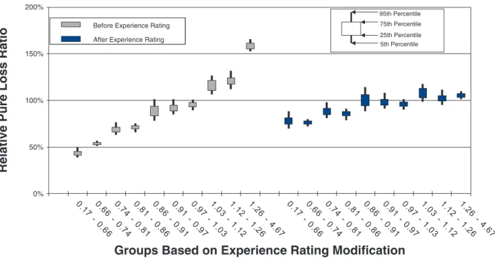
ferentiation between them. If risks were rated only on manual rates, then risks in the quintiles to the left would produce more favorable underwriting results.

The second set of bars in Figure 1 demonstrates that the combination of manual rates and the mod is equitable. The underwriting results are equal across the quintiles. Hence underwriting results are the same for risks with different mod values.

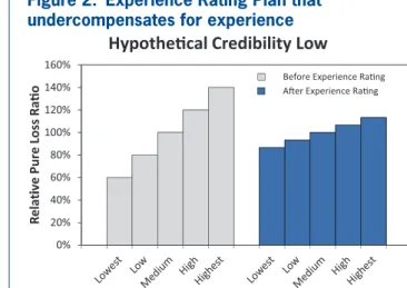
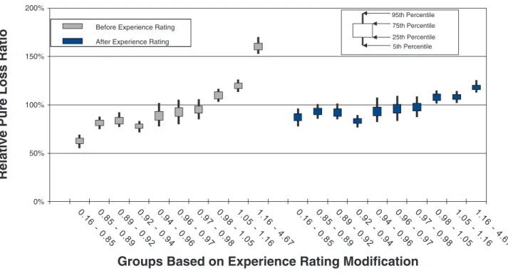
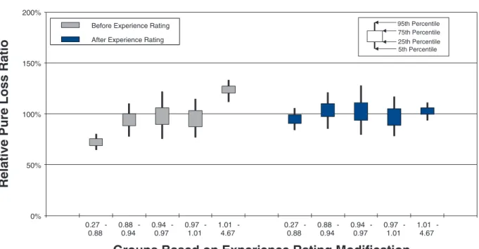
Figure 2 displays a hypothetical ERP with consider-able lift, as seen by the bars on the left side. The five bars on the right side demonstrate that the mod has not fully corrected for predictable differences in manual loss ratios. The rating plan does not charge risks with high mods enough and overcharges risks with lower mods. This inequity is generally the result of not assigning enough credibility to individual risk expe-rience. In contrast, Figure 3 displays a hypothetical ERP that over-corrects for predictable differences— this generally results from assigning too much cred-ibility to individual risk experience.

In cases where specific measures are needed to quantify how effectively the ERP is finding lift and achieving equity, the NCCI considers two statistics. The older quintile test statistic is B*/A*, where A* is the variance of the unmodified quintile pure loss ratios and B* is the variance of the modified quintile pure loss ratios: the variance in the pure loss ratios after application of the modification factors is divided by the variance in the pure loss ratios at manual rates. This traditional statistic measures equity or, perhaps quintiles for the policy year to which the experience

mod applies both before and after the mod is applied to manual expected losses. Several adjustments are made to reported actual losses and NCCI manual rates so that losses are on an ultimate basis and exclude both underwriting and loss adjustment expenses. A scale factor is also used to set total modified expected losses equal to total actual losses by risk hazard group within each state. This equalization isolates relative differences between risks, which the mod is designed to address, from issues of aggregate rate adequacy, which are addressed by manual rates levels.

2.2. Lift and equity

If the ERP can actually differentiate between risks then pure loss ratios calculated from manual rates should increase when moving from lower quintiles to higher quintiles. This increasing slope is called lift. The steeper the lift, the more value the mod offers in differentiating risks.

Including the mod in the calculation of expected losses should result in nearly equal pure loss ratios, or equity, across quintiles if the ERP is working well and there is sufficient data in each quintile. This flat-ness of the relative modified pure loss ratios reveals how well the mod achieves equity between risks.

Figure 1 displays an idealized hypothetical exam-ple. The bars on the left side of the chart demonstrate the concept of lift. The mod is able to differentiate between risks and the slope shows the degree of

dif-60% 80% 100% 120% 140% 160%

ive Pure Loss Rao

Before Experience Rang Aer Experience Rang

0% 20% 40%

Re

lati

Groups Based on Experience Rang Modificaon Hypothecal Credibility Opmal

Figure 1. Experience Rating Plan displaying lift and equity

60% 80% 100% 120% 140% 160%

Hypothecal Credibility Low

0% 20% 40%

Re

lati

Groups Based on Experience Rang Modificaon

(4)

risk has the same expected loss. σ2_{/n is the variance}

and σ n is the standard deviation in the overall pure loss ratio for a bin containing n homogeneous risks. As can be seen in Figure 4, the decreasing vari-ance as n increases results in a tighter curve clustered around the expected value.

The practical implication of this is that we expect for both manual and modified pure loss ratios the ran-dom observation error will be proportional to 1 n. Although the assumptions about homogeneity of risks are far from perfectly met in the real world, the departure will generally not cause this 1 n relation-ship to lose its practical value.

2.4. Systematic differences versus

random variation

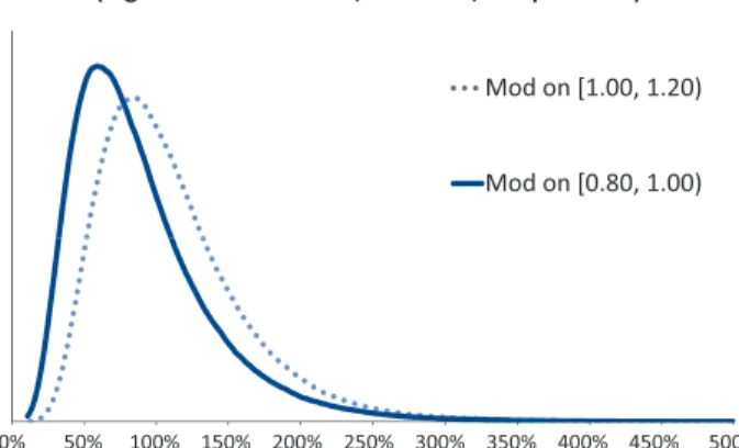
Individual quantiles should contain enough data so that the random variation of the manual pure loss ratios within quantiles is small compared to systematic dif-ferences in the underlying expected manual pure loss ratios between quantiles. As another hypothetical exam-ple, suppose that risks with mods uniformly distributed on the interval [0.80, 1.00) are compared to risks with mods uniformly distributed on the interval [1.00, 1.20). Figures 5a and 5b show, for interval sample sizes 1 and 100, respectively, hypothetical distributions for manual loss ratios for risks uniformly distributed across these two intervals, assuming individual risk loss ratios are lognormally distributed with mean equal to the mod value and 0.50 standard deviation.

more correctly, the movement towards equity with the ERP. Ideally it should be as close to zero as pos-sible. Note that B*/A* would be zero for Figure 1 because B*, the variance in the modified quintile loss ratios, is zero for this hypothetical example.

The newer quintile test statistic is sign(A-B) | A-B | 0.5_,

where A and B are equivalent to A* and B*, but may be calculated to include some extra variance due to boot-strapping the test, as will be discussed in section 3.1 This newer statistic measures how effectively the ERP is at finding lift and achieving equitable workers compensation rating. Ideally, it should be as large as possible. Using this new test statistic, Figure 1 trumps Figures 2 and 3 because all three have the same value for A but B takes on the smallest possible value of zero for Figure 1.

2.3. Sample size and the central

limit theorem

The central limit theorem says that the sum or aver-age of a large number of independent random vari-ables will be approximately normal. Even a highly skewed distribution such as the pure loss ratio for an individual risk will tend towards a normal distribu-tion if an average is computed over many risks. Fig-ure 4 illustrates this concept.

To simplify the discussion, assume that pure loss ratios for risks are independently and identically dis-tributed with mean µ and variance σ2_{and that each}

60% 80% 100% 120% 140% 160%

Hypothecal Credibility High

0% 20% 40%

Re

lati

Groups Based on Experience Rang Modificaon

Figure 3. Experience Rating Plan that

overcompensates for experience _{Probability Density of Sample Average}

(lognormal distribuon, CV = 50%)

Sample Size 1 Sample Size 10 Sample Size 100 Sample Size 1000

(5)

Figure 6 shows an idealized view of the dilemma. Here, we revisit the example from Figure 5b, break-ing up the two intervals, each with 100 sampled risks into four intervals, each with 50 sampled risks. First, note that we can safely ignore the contribution of variance of the mod within an interval to the variance of the loss ratio. The variance of the mod within the original two intervals of width 0.20 was 0.003 and for the split intervals of width 0.10 was 0.0008, triv-ial compared to the conditional variance of 0.25 for the loss ratio. So, there will be an increase of about 41% in the standard deviation of the overall loss ratio due to smaller sample size. Simultaneously, the dis-tance between the midpoints of the adjacent intervals has been cut in half. Consequently, the ratio of ran-dom variation to systematic variation in Figure 6 is about 282% of what it was in Figure 5b.

Note the substantial overlap in the distributions of actual pure loss ratios in the Figure 5a. There is a fair chance that the actual ratio for a risk from [0.80, 1.00) will exceed that for a risk from [1.00, 1.20), which would give misleading results about mod per-formance. One might conclude that the mod cannot effectively distinguish the loss potential of individ-ual risks. If there are more risks in each interval, as in Figure 5b, then the distinction is almost certainly shown in the observed loss ratios.

The systematic difference between the two previous intervals can be quantified as the differences between their midpoints of 0.90 and 1.10. Assuming that there are enough risks in the intervals so that the resulting distributions are approximately normal, standard devi-ations of manual loss ratios are a good way to charac-terize random variation. The choice of how small the random variation must be compared to the systematic difference is fairly subjective but not impractically ambiguous, as will be demonstrated in the next sections.

2.5. Tradeoffs in determining

the number of quantiles

More quantiles provide a more detailed look at how the plan is performing all along the range of mod val-ues. However, more quantiles will increase the random variation within each quantile because a fixed number of risks will be split into fewer risks per quantile. Worse still, more quantiles will simultaneously decrease the systematic differences between adjacent quantiles.

Probability Density of Sample Average (lognormal distribuon, SD = 0.50, sample size 1)

Mod on [1.00, 1.20) Mod on [0.80, 1.00)

0% 50% 100% 150% 200% 250% 300% 350% 400% 450% 500% 50% 60% 70% 80% 90% 100% 110% 120% 130% 140% 150%

Probability Density of Sample Average

(lognormal distribuon, SD = 0.50, sample size 100)

Mod on [1.00, 1.20) Mod on [0.80, 1.00)

Figures 5a and 5b. Random outcomes versus systematic differences

50% 60% 70% 80% 90% 100% 110% 120% 130% 140% 150%

Probability Density of Sample Average

(lognormal distribuon, SD = 0.50, interval sample size 50)

Mod on [0.90, 1.00) Mod on [0.80, 0.90) Mod on [1.00, 1.10) Mod on [1.10, 1.20)

(6)

nificance of noise-to-signal ratios using a normal distribution model. Note that this example shows the result of reducing the numerator, i.e., the noise, in the N/S ratio. The standard deviations of the normal curves become smaller moving from left to right and top to bottom in the figure. The distance between the means, i.e., the signal, is unchanged.

Table 1 shows the probabilities of reversals for a normal distribution model. By reversal we mean that the observed loss ratio for the higher interval is actu-ally lower than the observed loss ratio for the lower interval.

There is no precise objective standard for selecting a specific tolerance level for the N/S ratio. However, with consideration of Figure 7 and Table 1, a selec-tion of 0.25 for the N/S ratio tolerance level might

2.6. Noise-to-signal ratio

It is conceptually useful to think of random vari-ation in observed loss ratios as noise and the sys-tematic difference between the means of adjacent bins as signal. The ratio of random to systematic variation that we previously alluded to is explicitly defined and referred to as the noise-to-signal ratio (N/S) in (2.2).1

= = Noise

Signal N S

Standard deviation of random variations for an interval loss ratio Difference in expected

loss ratios between intervals

(2.2)

All other things equal, this ratio should be as small as possible. Figure 7 graphically illustrates the

sig-Noise-to-Signal = 1.00

Noise-to-Signal = 0.50

Noise-to-Signal = 0.25

Noise-to-Signal = 0.10

Figure 7. Noise-to-signal for normal distributions

1_{A formal mathematical definition of the N/S ratio could be:}

N/S = {(1/b)∑b

i=1(Var[LRi])1/2}/{(1/(b − 1)) ∑ib=−1 1| E [LRi+1]− E[LRi] |}

where LR_i is the actual loss ratio for the ith quantile and b is the number of quantiles. The numerator is simply the average of the standard devia-tions of the individual quantile loss ratios. The denominator measures the average “distance” between expected loss ratios of adjacent quantiles. Other definitions for N/S may be possible.

Table 1. Noise-to-signal ratios and ordering of pure loss ratios

Noise-to-Signal Ratio Probability of Reversal

1.00 0.2398

0.50 0.0786

0.25 0.0023

(7)

Solving for sample size n leads to (2.4).

N S (2.4)

2

2 3

n

(

R

)

b

(

)

= σ

Equation (2.4) shows, among other relations, that the amount of data needed increases as the cube of the number of quantiles: n ∝ b3_{. The ERP is}

cur-rently tested using a quintile test. A decile test would require eight times as much data for a comparable N/S ratio. Similarly, a test with 20 quantiles would require 64 times as much data.

3. Results and Discussion

3.1. Bootstrapping empirical data

demonstrates effects of number

of quantiles

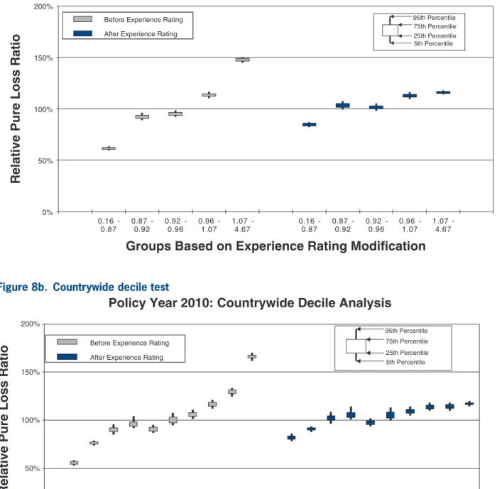
To measure the noise associated with the relative pure loss ratios in a quintile test, NCCI bootstraps the underlying data. The data set of risks used for a par-ticular test is resampled with replacement 100 times. Each time, the quintile test loss ratios are recalculated. A candlestick chart illustrates the 5th, 25th, 75th, and 95th percentiles of the bootstrapped relative pure loss ratios. The vertical spread of the quintile bars is indica-tive of the noise in the test, and the difference in the vertical location between adjacent candles is indica-tive of the signal in the test. Consider the following bootstrap quintile and decile tests for policy year 2010:

• Figures 8a and 8b are countrywide, which includes 886,976 individual risks.

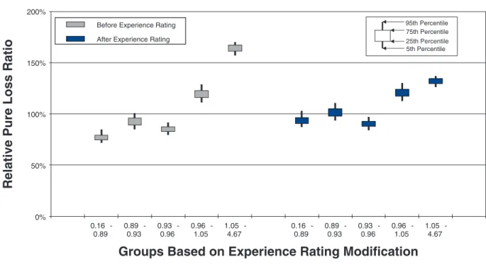
• Figures 9a and 9b are countrywide for risks whose policy period expected pure loss ranges from 1k to 10k, which includes 467,887 individual risks. • Figures 10a and 10b are countrywide for risks whose

policy period expected pure loss ranges from 100k to 1m, which includes 18,692 individual risks. • Figures 11a and 11b are for a large state, which

includes 62,629 individual risks.

• Figures 12a and 12b are for a small state, which includes 10,943 individual risks.

Comparison between the quintile and decile tests illustrates an increasing N/S ratio as the number of be judged reasonable to provide clarity of

distinc-tion in loss ratios between adjacent quantiles and a low probability of reversals between adjacent quan-tile intervals. So, the “optimal” number of quanquan-tiles is beginning to emerge. If we can estimate the N/S ratio as a function of the number of quantiles, then the maximum number of quantiles within our N/S tolerance will be that “optimal” number.

2.7. The number of quantiles

and data requirements

To address the question of the number of quantiles, the N/S signal ratio can be estimated by a formula in terms of the following quantities:

b= number of quantiles

σ2=_{variance of the manual pure loss ratio for a single}

risk

n=number of risks tested

R= a constant corresponding to the “spread” or “vari-ation” of mods

We will assume risks are all the same size. This is a reasonable simplifying starting assumption, but in reality risk sizes and the variances of their loss ratios span across orders of magnitude for the ERP. The resulting formula will be validated, or invalidated, for the general context using empirical data.

The standard deviation for the loss ratio in a single quantile will be σ n b= b

(

σ n

)

. Again, we will ignore variation in the loss ratio due to mod differ-ence within quantiles, as this usually contributes a very small part of the total random variation.

If there are more quantiles, then the differences between the expected values for the mods of adjacent quantiles is smaller. If the number of bins is doubled, then these differences should be approximately cut in half. A reasonable rule of thumb is that the typi-cal difference is inversely proportional to b, that is, equal to R/b.

Putting the pieces above together, the N/S ratio for-mula leads to (2.3).

N S (2.3)

3

b n

R b R

b n

(

)

(

)

= σ = σ

(8)

Policy Year 2010: Countrywide Quintile Analysis

0% 50% 100% 150% 200%

0.16

-0.87 0.87 -0.92 0.92 -0.96 0.96 -1.07 1.07 -4.67 0.16 -0.87 0.87 -0.92 0.92 -0.96 0.96 -1.07 1.07 -4.67

Relative Pure Loss Ratio

Groups Based on Experience Rating Modification

Before Experience Rating After Experience Rating Before Experience Rating After Experience Rating

5th Percentile 95th Percentile 25th Percentile 75th Percentile Before Experience Rating

After Experience Rating

Figure 8a. Countrywide quintile test

Relative Pure Loss Ratio

Policy Year 2010: Countrywide Decile Analysis

0% 50% 100% 150% 200%

Groups Based on Experience Rating Modification

5th Percentile 95th Percentile

25th Percentile 75th Percentile Before Experience Rating

(9)

Policy Year 2010: Prospective Period Pure Expected Losses 1K - 10K Quintile Analysis

0% 50% 100% 150% 200%

0.16

-0.89 0.89 -0.93 0.93 -0.96 0.96 -1.05 1.05 -4.67 0.16 -0.89 0.89 -0.93 0.93 -0.96 0.96 -1.05 1.05 -4.67

Groups Based on Experience Rating Modification

Before Experience Rating

After Experience Rating Before Experience Rating

Relative Pure Loss Ratio

Figures 9a. Countrywide small risk quintile test

Policy Year 2010: Prospective Period Pure Expected Losses 1K - 10K Decile Analysis

0% 50% 100% 150% 200%

Groups Based on Experience Rating Modification

5th Percentile 95th Percentile

Relative Pure Loss Ratio

(10)

Policy Year 2010: Prospective Period Pure Expected Losses 100K - 1M Quintile Analysis

0% 50% 100% 150% 200%

0.17

-0.74 0.74 -0.86 0.86 -0.97 0.97 -1.12 1.12 -4.67 0.17 -0.74 0.74 -0.86 0.86 -0.97 0.97 -1.12 1.12 -4.67

Groups Based on Experience Rating Modification

Relative Pure Loss Ratio

Figure 10a. Countrywide large risk quintile test

Policy Year 2010: Prospective Period Pure Expected Losses 100K - 1M Decile Analysis

0% 50% 100% 150% 200%

Groups Based on Experience Rating Modification

Before Experience Rating After Experience Rating Before Experience Rating

After Experience Rating _{5th Percentile}

95th Percentile

Relative Pure Loss Ratio

(11)

Relative Pure Loss Ratio

Policy Year 2010: Large State Quintile Analysis

0% 50% 100% 150% 200%

0.16

-0.89 0.89 -0.94 0.94 -0.97 0.97 -1.05 1.05 -4.67 0.16 -0.89 0.89 -0.94 0.94 -0.97 0.97 -1.05 1.05 -4.67

Groups Based on Experience Rating Modification

Figure 11a. Large state quintile test

Relative Pure Loss Ratio

Policy Year 2010: Large State Decile Analysis

0% 50% 100% 150% 200%

Groups Based on Experience Rating Modification

95th Percentile

(12)

Relative Pure Loss Ratio

Policy Year 2010: Small State Quintile Analysis

0% 50% 100% 150% 200%

0.27

-0.88 0.88 -0.94 0.94 -0.97 0.97 -1.01 1.01 -4.67 0.27 -0.88 0.88 -0.94 0.94 -0.97 0.97 -1.01 1.01 -4.67

Groups Based on Experience Rating Modification

Figure 12a. Small state quintile test

Relative Pure Loss Ratio

Policy Year 2010: Small State Decile Analysis

0% 50% 100% 150% 200%

Groups Based on Experience Rating Modification

95th Percentile 25th Percentile 75th Percentile Before Experience Rating

(13)

bins increases. Since the N/S ratio should also change in proportion to 1 n, where n is the number of risks, all other things equal (which they are not), we would expect the N/S to increase going from Figures 8a and 8b to Figures 12a and 12b. In fact, such a pattern is clearly evident. However, between tests using the same number of quantiles but different data, the random vari-ation in the loss ratio per individual risk may vary, and will certainly decrease going from the small risks in Figures 9 to the large risks in Figures 10. Another thing that can change as the underlying data set changes is the typical signal difference between the quantiles.

The general consistency between the patterns observed in these charts and what we expect from the N/S ratio model provides a reasonable validation of the model as a practical tool. The next section shows bootstrapped estimates of the N/S ratios for the ten charts.

3.2. Noise-to-signal ratio

The noise-to-signal ratio (N/S) was introduced in equation (2.2) of section 2.6.

= = Noise

Signal N S

Standard deviation of random variations for an interval loss ratio Difference in expected

loss ratios between intervals

(2.2)

Although an explicit formula for calculating noise-to-signal ratios was presented in equation (2.3), the ratios can also be estimated by bootstrapping empiri-cal data. Noise-to-signal ratios corresponding to the bootstrapping results used to create the charts in section 3.1 are displayed in Table 2. As expected,

Table 2. Bootstrapped estimates of noise-to-signal ratios Noise-to-Signal _{N/S Decile/}

N/S Quintile Quintile Decile

Countrywide (C/W) 0.086 0.229 2.67

C/W $1K–$10K 0.203 0.499 2.46

C/W $100K–$1,000K 0.128 0.354 2.75

Large State 0.192 0.482 2.51

Small State 0.748 1.973 2.64

the noise-to-signal ratios are significantly higher for deciles than quintiles. The last column of the table displays the ratio of noise-to-signal ratios for deciles to those of quintiles.

Equation (2.3) shows that N S 3 b

∝ where b is the number of quantiles. Comparing deciles and quin-tiles with this proportionality yields a value not too far from those in the last column of Table 2.

÷

= ÷ = =

N S Deciles N S Quintiles

103 53 23 2.83.

The theoretical value 2.83 is somewhat greater than values in the table because the experience modi-fication factors spread out in the two tails of the mod distribution. This would not happen if the mods were uniformly distributed over a range.

3.3. Measuring lift and equity

At the end of section 2.2 two statistics were intro-duced: (1) B*/A* (smaller is better) is a measure of how effectively the ERP achieves equity, and (2) sign(A-B) | A-B | 0.5_{(larger is better) is a}

combina-tion measure that increases with more lift, A is larger, and increases with more equity, B is smaller. A* is the variance of the unmodified pure loss ratios and B* is the variance of the modified pure loss ratios across the quantile groups. The quantities without the * are similar quantities but may include some additional variance from bootstrapping.

Table 3 displays these statistics for the 2010 pol-icy year data that was used to create the prior ten bootstrapping charts. The first column of numbers, B*/A*, shows that the ERP makes considerable prog-ress towards achieving equity because the variance in pure loss ratios is much smaller for the modified pure loss ratios than the unmodified pure loss ratios. For example, the variance in the countrywide modified pure loss ratio quintiles is only 14.9% of the vari-ance in the unmodified quintiles. The second column shows that the ERP is finding lift and moving towards more equitable rating.

(14)

for PY 2010 highlight the need for increased effec-tive credibility that prompted NCCI’s increases in the split point beginning in 2013, from $5,000 to $10,000 in year one, $13,500 in year two, and $15,000 plus two years of inflation adjustment in year three. Fur-ther routine increases based on severity indexation will follow.

3.4. Some hypothetical examples

Appendix A develops the rule of thumb, shown in (3.1), to estimate σ/R in terms of the credibility Z for an individual risk loss ratio. This is potentially par-ticularly useful, as Z can act as a reasonable measure of risk size, though not on a proportional scale.

1 1

12 (3.1)

2

R

Z

σ = −

However, before progressing too far we must recall that in principle a Z credibility value such as this, although it includes useful information about σ/R, is qualitatively very different from the Z_p and Z_e values found in the experience rating. This Z value would:

1. Estimate the true underlying mean for a single pol-icy year using that polpol-icy year’s losses, rather than using prior policy years’ experience to predict the true mean for a future policy year.

2. Cover all losses unlimited. 3. Use only one year of losses.

So, much caution must be used in attempting to apply it to the very different situation of the ERP. Unfortunately, there is no clear way to relate Z to the readily available, but fundamentally very differ-ent, Z_p and Z_e. More generally, there is probably no good way to determine such a Z that would directly apply to the context of the NCCI ERP. Statement 1 suggests Z should be higher than Z_p, but 2 and 3 suggest Z should be lower than Z_p. Since higher Z implies lower σ/R and hence lower N/S, it is pru-dent to err on the side of a lower Z. So, on balance, it is not unreasonable to speculate that Z should be on the same order as Z_p, but somewhat lower, per-haps Z ≈ Z_p/2. Ultimately, any N/S model resulting from whatever relationship we may assume can be validated or invalidated using empirical data along the lines we followed in section 3.1. Table 4 explores what different values for Z, n, and b imply for the N/S ratio. The N/S ratios in the table can be computed by substituting the right-hand side of equation 3.1 for σ/R in equation 2.3.

The formulas for Z_e and Z_p vary by state and over time, according to a fairly complicated formula that is a function of experience period expected losses rather than policy period pure expected losses. How-ever, the values in Table 4 would be roughly in the ballpark for recent years.

The conjecture Z ≈ Z_p/2 together with Table 5 suggest that Z would be around 3% to 20% for ures 9a and 9b and around 40% to 45% for Fig-ures 10a and 10b.

Next, recall that Figure 9 had a sample size approaching half a million risks and Figure 10 had a sample size a bit under 20,000. From Table 4 we can see that both Figures 9 and 10 would be expected to be well within the acceptable N/S for the quintile. The deciles test would be expected to be around the maximum N/S ratio. This is roughly the situation we see in the charts and therefore Z≈ Z_p/2, although not founded in any sort of solid mathematics or logic, is still empirically validated to be in the ballpark and therefore practically use-ful within broad limits.

Table 3. Statistical measures of lift and equity Statistics

B*/A* sign(A-B)| A-B| 0.5

Countrywide Quintile 0.149 0.261

Countrywide Decile 0.140 0.265

Countrywide Small Risks Quintile 0.265 0.272

Countrywide Small Risks Decile 0.259 0.284

Countrywide Large Risks Quintile 0.105 0.296

Countrywide Large Risks Decile 0.107 0.309

Large State Quintile 0.144 0.232

Large State Decile 0.150 0.239

Small State Quintile 0.044 0.157

(15)

4. Conclusions

The number of quantiles selected for a meaningful test of predictive performance of the NCCI Experi-ence Rating Plan is constrained by the ratio of noise-to-signal. If this ratio is not kept below a reasonable threshold, which is subjective but can be sensibly selected somewhere in the neighborhood of 0.25, the results of the quantile test will be unclear. In a sense, the “optimal” number of quantiles is the largest num-ber that produces a N/S ratio under this threshold. The N/S ratio is proportional to the standard devia-tion of observed loss ratios for individual risks and the 1.5 power of the number of quantiles. The N/S

ratio is inversely proportional to the variation in mod values and the square root of the number of risks in the data. Consequently, the data required to maintain a given N/S ratio is proportional to the cubic power of the number of quantiles. This huge data penalty in test resolution for increasing the number of quan-tiles explains the use of a relatively small number of quantiles, exactly five in the quintile test, for testing the NCCI Experience Rating Plan. These and other implications of this N/S ratio can be demonstrated consistently for both empirical tests of the ERP and hypothetical examples.

Appendix A. A Connection

Between Noise-to-Signal Ratio

and Credibility

Suppose a single credibility Z value, which can be any value in (0%, 100%) not necessarily based on any sound credibility model, is used on the total unlimited policy year loss ratio L to estimate a non predictive individual risk modification factor. That is, a risk’s actual loss ratio in a single year is used to estimate

Table 5. Approximate recent ERP credibility by risk size

Policy Period Approximate Recent ERP Credibility

Pure Premium Zp Ze

1,000 5% 0%

10,000 40% 2%

100,000 80% 10%

1,000,000 90% 40%

Table 4. Noise-to-signal by Z credibility Noise to Signal <= 0.25 Shaded

Z Credibility = 50%

Sample Size—>

Quantiles 100 1,000 10,000 100,000 1,000,000

2 0.14 0.04 0.01 0.00 0.00

5 0.56 0.18 0.06 0.02 0.01

10 1.58 0.50 0.16 0.05 0.02

20 4.47 1.41 0.45 0.14 0.04

100 50.00 15.81 5.00 1.58 0.50

Z Credibility = 10%

Sample Size—>

Quantiles 100 1,000 10,000 100,000 1,000,000

2 0.81 0.26 0.08 0.03 0.01

5 3.21 1.02 0.32 0.10 0.03

10 9.08 2.87 0.91 0.29 0.09

20 25.69 8.12 2.57 0.81 0.26

100 287.23 90.83 28.72 9.08 2.87

Z Credibility = 25%

Sample Size—>

Quantiles 100 1,000 10,000 100,000 1,000,000

2 0.32 0.10 0.03 0.01 0.00

5 1.25 0.40 0.13 0.04 0.01

10 3.54 1.12 0.35 0.11 0.04

20 10.00 3.16 1.00 0.32 0.10

100 111.80 35.36 11.18 3.54 1.12

Z Credibility = 5%

Sample Size—>

Quantiles 100 1,000 10,000 100,000 1,000,000

2 1.63 0.52 0.16 0.05 0.02

5 6.45 2.04 0.64 0.20 0.06

10 18.23 5.77 1.82 0.58 0.18

20 51.58 16.31 5.16 1.63 0.52

(16)

the difference between adjacent quantiles would be 0.035 in this situation.

References

Dorweiler, P., “A Survey of Risk Credibility in Experience Rating,” Proceedings of the Casualty Actuarial Society 21, 1934, p. 1.

Gillam, W. R., “Parametrizing the Workers Compensation Expe-rience Rating Plan,” Proceedings of the Casualty Actuarial

Society 79, 1992, p. 21–56.

Meyers, G. G., “An Analysis of Experience Rating,”

Proceed-ings of the Casualty Actuarial Society 72, 1985, p. 278. NCCI (National Council on Compensation Insurance),

Expe-rience Rating Plan Manual for Workers Compensation and Employers Liability Insurance, updated annually.

Venter, G. G., “Experience Rating—Equity and Predictive Accu-racy,” NCCI Digest, April 1987, Vol. II, Issue I, pp. 27–35.

Abbreviations and Notations

ERP—experience rating plan

NCCI—National Council on Compensation Insurance N/S—noise-to-signal ratio

A, A*—variance of un-modified quintile pure loss ratios

B, B*—variance of modified quintile pure loss ratios

b—number of quantiles

L—unlimited policy year loss ratio for a risk

n—number of risks

R—spread in modification factor values

σ2_{—variance in pure loss ratio for one risk} σˆ2

L—actual sample variance of observed loss ratios Zp—primary credibility for an experience rated risk Ze—excess credibility for an experience rated risk Z—credibility for an individual risk

Table A1. Differences between decile means for a lognormal distribution with mean 1.00 and standard deviation 0.10

Decile Mean Difference

1st 0.836

2nd 0.897 0.061

3rd 0.930 0.033

4th 0.957 0.027

5th 0.983 0.025

6th 1.008 0.025

7th 1.034 0.027

8th 1.065 0.030

9th 1.104 0.040

10th 1.186 0.082

its own true mean loss ratio for that same year. The sample variance in such a mod would be (A.1).

1

1 1 1

1 ˆ (A.1) 1 2 2 1 2 2 2

n Z L Z L Z L Z L

Z

n L L

Z i i n i i n L

∑

[

(

)

]

(

)

( ) ( ) − + − − + − = − − = σ = =

where σˆ2

L is the actual sample variance of the observed

loss ratios. The remaining or “random” part of the sam-ple variance is (A.2).

1 2 ˆ2 (A.2)

Z L

(

−

)

σ

Although a quantile test would be meaningless in this non-predictive situation, we can estimate a ratio σ/R in the N/S formula (2.3). (A.2) can be used as an estimate of σ2_{and (A.1) can be used to derive an}

esti-mate for R. As a simplification, assume that mods are effectively uniformly distributed across an interval of width R. For a uniform distribution the difference between the means of mods in adjacent quantiles, or signal, where mods are split into b quantiles would be R/b. This is the key property of R as used in (2.3). Equating the variance expression for a uniform dis-tribution with (A.1) leads to (A.3).

12 ˆ (A.3)

2

2 2 R

Z L

= σ

This would lead to (A.4).

1 ˆ 12 ˆ 1 1 12 (A.4) 2 2 2 2 2 R Z Z Z L L