EXAMINING THE ROLE OF NETWORK STRUCTURE IN HIV TRNAMISSION AMONG PEOPLE WHO INJECT DRUGS IN THE PHILIPPINES: A TALE OF TWO CITIES
Nalyn Siripong
A dissertation submitted to the faculty at the University of North Carolina at Chapel Hill in partial fulfillment of the requirements for the degree of Doctor of Philosophy in the Department of Epidemiology
in the Gillings School of Global Public Health.
Chapel Hill 2017
iii ABSTRACT
Nalyn Siripong: Examining the Role of Network Structure in HIV Transmission among People who Inject Drugs in the Philippines: A Tale of Two Cities
(Under the direction of Brian W. Pence)
While HIV growth has slowed globally, new HIV epidemics among people who inject drugs (PWID) continue to emerge [1-4]. These epidemics are marked by periods of unusually rapid growth, where HIV increases from virtually 0% to 20-50% within 3-6 years [5-6]. In concentrated epidemics, HIV epidemics among PWID could precipitate larger-scale heterosexual epidemics [7-10], which further underscores the urgent need to find effective ways to reach and deliver prevention services to PWID.
We studied the emergence of HIV among PWID in two cities in the Philippines. The epidemic began in Cebu City, where HIV prevalence grew from 0.6% in 2009 to 50% in 2010 [11]. Expanded surveillance in neighboring Mandaue City found more limited spread of infection, with HIV prevalence reaching only 3.5% in 2011[12], rising to 38% in 2013 [13]. We used exponential random graph models (ERGMs) to simulate network structures and assess whether differences in network structure could explain variation in HIV prevalence patterns in the two cities. We further analyzed genetic sequencing data to consider the extent of overlap or linkage between networks.
iv
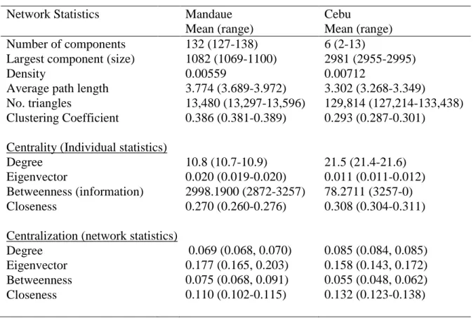
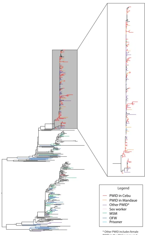
v 10.8), lower clustering (0.29 v 0.39), and shorter average paths (3.3 v 3.8), all of which would facilitate rapid spread of infection across the network. A phylogenetic tree showed high bootstrap support for a large cluster of HIV infections (N = 172), predominantly from PWID from Cebu and Mandaue (85%), which suggests that HIV infection in the two cities arose from a common source infection.
v
ACKNOWLEDGEMENTS
This is not my work, but a true collaboration in every sense of the word. I could not have the idea (or the data!) were it not for Genesis Samonte, my ‘ate’ and mentor and friend. I could not conduct the sequencing analysis without Ivo Sah Bandar, and I would not
understand any of what I was doing without the guidance of Ann Dennis. I could not
understand network concepts without Jim Moody, Jeff Smith, and Jake Fisher. I would have understood anything about respondent-driven sampling without Ashton Verdery. I would never appreciate the importance of modeling without the mentorship and teachings of Kim Powers and Annelies van Rie. I never could have completed this document (and graduated) without my adviser, Brian Pence, who . And I never would have kept my sanity without the support of my friends - especially Christine Gray, Marissa Seamans, and Joann Gruber – and my family, the ‘other’ Dr. Siripongs, and my partner, Edward Levicoff.
vi
TABLE OF CONTENTS
LIST OF TABLES ... ix
LIST OF FIGURES ...x
CHAPTER 1: SPECIFIC AIMS ...1
CHAPTER 2: BACKGROUND AND SIGNIFICANCE...4
Epidemiology of HIV among people who inject drugs ... 4
Understanding the disease dynamics from network theory and modeling ... 6
Networks among people who inject drugs (PWID) ... 10
Use of PWID network structures to estimate impacts on HIV infection ... 12
Significance ... 17
Innovation ... 18
CHAPTER 3: METHODS ...19
Study Population ... 19
Sampling methods: a brief description of RDS ... 20
RDS implementation ... 23
Estimating population characteristics ... 25
RDS Homophily ... 25
Measuring the ego-network configuration distribution ... 26
Simulating networks ... 27
vii
Aim 1 Limitations ... 37
Building the consensus sequences ... 38
Sequence alignment ... 39
Phylogenetic tree construction ... 40
Aim 2 Limitations ... 42
CHAPTER 4: IDENTIFYING NETWORK STRUCTURES THAT IMPACT HIV TRANSMISSION DISEASE DYNAMICS IN THE PHILIPPINES ...44
Introduction ... 44
Methods ... 45
Results ... 52
Discussion ... 54
Figures and Tables ... 57
CHAPTER 5: A PHYLOGENETIC ANALYSIS OF EMERGING EPIDEMICS AMONG PEOPLE WHO INJECT DRUGS IN THE PHILIPPINES ...63
Introduction ... 63
Methods ... 64
Results ... 68
Discussion ... 70
Conclusions ... 72
Figures and Tables ... 74
CHAPTER 6: DISCUSSION ...77
Aim 1: Evaluating the potential impact of network structures among PWID on HIV transmission ... 78
Summary of Findings ... 78
Public Health Significance ... 79
viii
Future Research ... 81
Aim 2: A phylogenetic analysis of emerging epidemics among people who inject drugs in the Philippines ... 82
Summary of Findings ... 82
Public Health Significance ... 82
Limitations ... 83
Future Research ... 84
Conclusions ... 84
ix
LIST OF TABLES
Table 1. Over several waves of infection, characteristics in an RDS sample will
approach the true population characteristics. ... 21 Table 2. Homophily is calculated based on the expected ties under random mixing
(left) compared to observed mixing (right). ... 26 Table 3. Building a consensus sequence usually means taking the majority base
present at each site. ... 38 Table 4. Demographic and behavioral characteristics of the sample, weighted using
Gile’s successive sampling estimator [95]. ... 57
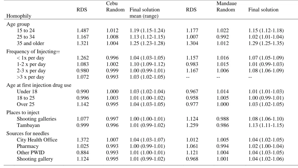
Table 5. Homophily of characteristics of interest. ... 58 Table 6 (a/b). Comparison of RDS-weighted characteristics and random network
characteristics in Cebu (a) and Mandaue (b). ... 59 Table 7. Comparison of homophily from RDS, random network and the final
solution shows homophily from our solutions are somewhat close to
empirical estimates. ... 61 Table 8. Summary network statistics of simulations in Cebu and Mandaue. ... 62 Table 9. Comparison of behavioral characteristics, by PCR amplification status, in
Cebu and Mandaue. ... 75 Table 10. Composition of the main transmission cluster (N=172), by HIV exposure
x
LIST OF FIGURES
Figure 1. Conceptual diagram describing how networks impact risk of HIV infection. ... 6 Figure 2. RDS samples will approach true population estimates, whether our seeds are
all in group A (left) or group B (right). ... 21 Figure 3. Ego-network configurations observed from RDS data collected in our survey. ... 27 Figure 4. Three components make up this network of 12 people; component A is the
largest connected component, including 58% (7 out of 12 individuals) of the
network. ... 33 Figure 5. Adding one tie to a network changes the clustering coefficient, but in
unpredictable ways. ... 36 Figure 6. Insertion of blank spaces can be necessary to align sequences with each other. .... 39 Figure 7. Best maximum likelihood (ML) phylogenetic tree of all 395 sequences in
the Philippines with 1,000 bootstrap replicates. Branches are colored by mode of transmission. The large cluster of 172 sequences has a bootstrap support of 97% and contains almost all sequences from PWID in Cebu and
1
CHAPTER 1: SPECIFIC AIMS
Over 11% of the 14 million people who inject drugs (PWID) worldwide are infected with HIV [14]. Most HIV epidemics in injection drug using populations are marked by rapid spread of infection, with prevalence rates in some communities rising from 0% to 50% in less than a year [6]. Given the high disease burden and susceptibility to rapid epidemic outbreaks, understanding HIV transmission dynamics among injection drug using populations is
critically important.
Injection epidemics are characterized by an initial rapid increase in HIV incidence followed by a plateau at some steady-state HIV prevalence. Transmission may be interrupted or facilitated through injecting behaviors like needle sharing and injecting frequency, which are the focus of most prevention efforts among injecting drug users. Yet network structure, or an injection drug user’s choice of injecting partners, may also strongly influences the spread of infection. Limitations in data and analytic methods have precluded use of network
information to target and design more effective prevention interventions.
Two distinct HIV outbreaks among injecting drug users in two neighboring
communities in the Philippines offer a unique opportunity to disentangle the contributions of individual behaviors and network structure on transmission dynamics. In Cebu City, HIV prevalence among people who inject drugs rapidly expanded from 0% in 2007 and 0.6% in late 2009 to 50% in 2010 and 53% in 2011 [11]. In neighboring Mandaue City, HIV
2
in 2013 [11-13]. PWID in both cities exhibited risky injecting behaviors, with a majority of people sharing drugs and injecting equipment in both cities. Identifying differences in the network structures between the cities may explain the differences in observed HIV spread in these two cities.
We hypothesize that the networks of PWID in Cebu City and Mandaue have different network structures, which explains the differences in HIV prevalence in the two cities.
Our specific aims are:
Aim 1: Compare network structure in Cebu City and Mandaue to identify important differences that correlate with differences in HIV prevalence.
Surveillance data were collected on a network of injecting drug users using respondent-driven sampling (RDS) recruitment methods. We will use the network-related information collected in this survey to map the injecting drug user networks in the two cities. We will compare network structures using statistics on component size, homophily, social distance, and clustering. To do this, we will simulate a network from an exponential random graph model (ERGM) aligned with initial network parameters, using three primary network measures: degree, homophily and clustering.
Aim 2: Examine phylogenetic clustering of HIV infections detected in Cebu City and Mandaue.
3
phylogenetic trees at a finer level of detail, we may find that most of the transmission is happening within each city, as opposed to across the two city boundaries.
4
CHAPTER 2: BACKGROUND AND SIGNIFICANCE Epidemiology of HIV among people who inject drugs
Among the estimated 12-14 million people who inject drugs (PWID) worldwide, 1.6 million (11%) are infected with HIV [14]. HIV infection presents a serious disease burden among PWID populations, with HIV prevalence exceeding 40% in countries across Southeast Asia, including Thailand and Indonesia [15-17]. In these concentrated epidemic settings, HIV epidemics among IDUs precipitate larger-scale heterosexual epidemics [7-10], which further underscores the urgent need to find effective ways to reach and deliver
prevention services to injecting drug users.
A striking and unique feature of PWID epidemics is the rapid HIV growth, from virtually 0% prevalence to a steady-state level of 20-50% HIV prevalence within 3-6 years. This transition has been characterized by an initial period of very high HIV incidence, with rates reaching 12.5 cases per 100 person-years [10]. As an increasing number of injecting drug users became infected, the pool of uninfected and susceptible PWID remaining is depleted. As the pool of susceptible PWID decreases, the incidence rate fall to rates as low as 2.4 cases per 100 person years [18] and settle at a rate equal to the turnover rate in the
injecting drug user population. In rare cases, adoption of safer injecting practices among new injectors can stop spread and reduce overall prevalence [19].
5
infection has been documented in many PWID populations [21], but other communities maintain low or undetectable HIV levels, despite persistent needle sharing [22,23]. We explore whether network structures may offer an explanation for unusual or unexpected patterns of HIV transmission in communities of people who inject drugs.
This dissertation explores the influence of network structures on transmission dynamics, using surveillance data from PWID in two neighboring cities in the Philippines: Cebu and Mandaue. In Cebu City, HIV prevalence among people who inject drugs rapidly expanded from 0% in 2007 and 0.6% in late 2009 to 50% in 2010 and 53% in 2013 [11]. In Mandaue, early signs suggested limited spread of infection, as HIV prevalence had reached only 3.5% in 2011 [12]. HIV prevalence grew in Mandaue, but the spread of infection was slower and its reach was limited, with just 38% HIV prevalence in 2013 [13]. PWID in both cities exhibited high-risk behaviors, with a majority of people sharing drugs and injecting equipment. Thus, identifying differences in the network structures between the cities and assessing the impacts of network structure on transmission of infection may offer insights to understanding factors that impact the patterns of disease spread in these two cities.
Aim 1: Importance of networks for disease transmission
6
networks influence decisions to share injecting equipment and ultimately how they may influence disease risk.
Figure 1. Conceptual diagram describing how networks impact risk of HIV infection.
Understanding the disease dynamics from network theory and modeling
Networks may alter perceived risk of infection in at-risk populations. For example, a person with a single sex partner appears to be at low risk, but may still be connected to a larger sexual network [24]. Similarly, an individual with multiple concurrent partners would typically appear high-risk, but actual risk of infection may be low if each of his or her partners was monogamous. In the absence of empirical data on networks among individuals at risk for HIV, modeling and simulation studies have offered a better understanding of how network structures may affect contact patterns and disease transmission.
Early simulations approximated network structure by modeling differential mixing patterns among people with different contact rates [25,26], following on work identifying the role of core groups in the transmission of sexually transmitted infections [27]. These studies show that homogenous mixing by activity group (i.e., people with many sex partners choose partners who also have many sex partners) would yield faster epidemic spread, but that in the long run, infection would remain more contained than under heterogeneous mixing
conditions. However, these models still assume random selection of sexual partners within HIV exposure
Injec ng behaviors
social context network structure
7
each group – an assumption that does not typically hold in most empirical sexual or social networks.
Further adaptation of ordinary differential equations (ODE) approximate network effects through two parameters: degree and clustering [28]. Degree is simply the average number of connections a person has. Clustering refers to how frequently closed triangles are observed when three people are connected to each other on the network. Although largely hypothetical, these simulations show how network structures could impact transmission dynamics. Epidemics were less likely to take hold in networks with low degree or high clustering, as both of these measures reduced the effective contact rate. The impacts of clustering were amplified in networks with low degree.
Although increasing average degree was found to be important for promoting disease spread, degree distribution can vary widely even while holding average degree constant. Several types of degree distribution and their implications for transmission modeling have been reviewed [29]. In latticed networks, individuals are equally spaced across the network and each person is connected to his or her nearest neighbors, resulting in a relatively constant degree distribution. This network is highly clustered, and risk of disease would be strongly associated with distance from the initial infection. So-called “small-world” networks have degree distributions similar to lattice networks, but their clustered structure is slightly modified so that a few random long-range ties are formed, which creates opportunities for infection to quickly jump and spread across a network in a less rigid manner [29-31].
8
approximate scale-free degree distributions [32-34]. One feature of scale-free networks is that most people have very few (one or two) connections so that the bulk of the distribution is at the low end of the distribution, and only one or two people are in the tail of the
distribution, connected to hundreds of others. These high-degree individuals could be considered analogous to the super-spreaders or core groups in epidemics [29,35], and simulations of transmission over scale-free networks often result in epidemics where infection is concentrated around those people with the highest degree [35,36].
Scale-free networks may not be the only relevant degree distribution for
understanding transmission of infection. Some argue that this may not be the best distribution to describe these empirical networks [37,38]. Moreover, knowing the degree distribution does not necessarily give us sufficient information to predict how infection would be transmitted over a network. Holding degree distribution constant, other network
characteristics can vary considerably, with important consequences for disease dynamics. Increases in clustering, for example, can reduce the growth of the epidemic by creating small inter-connected groups that are only weakly connected to other parts of the network [39]. Average path length on different networks has also explained observed variation in disease dynamics, even after accounting for degree distribution and clustering [40].
Several studies have collected information to explicitly identify ties among
9
increased clustering, which would make the network more robust to sustained transmission of infection [42].
Recognizing the wide variation possible even within a constrained set of network parameters (e.g., degree distribution), much work on modeling of disease transmission over networks has adopted a two-part approach, which both estimates the network formation process and simulates transmission of infection over that network. Several studies simulating transmission over sexual networks observed in empirical data found that these networks were susceptible to breaks in transmission [41,43]. Larger networks simulated from casual contact or traffic patterns suggested that more densely connected networks were not subject to the same vulnerabilities [33]. Simulations based on empirical data on social networks estimate the range of potential network realizations for a given set of network characteristics, as well as their consequences for transmission dynamics [44,45].
Pairwise-formation models approximated transmission over agent-based models by considering each tie in the network as a separate observation. While some of these models can reproduce disease dynamics consistent with the agent-based models, they do not record the disease and contact history of individuals on the network [29,46]. These models can incorporate some of the effects of network structures on transmission [47], but they do not reconstruct the complete network, and thus may not be able to identify the roles of larger structures (i.e., those made up of four or more nodes).
10
combination of network characteristics has the greatest influence on disease transmission dynamics.
Networks among people who inject drugs (PWID)
Network studies of PWID consider both the effects of local networks on drug use practices and the impacts of network structures on an individual’s exposure to infection. Local networks consider an individual’s direct social ties and shared bonds or trust can influence his or her risk behaviors. When networks were described more comprehensively, large structures, such as bi-components (cycles), could be identified and their impacts assessed by estimating whether membership to these structures was associated with higher disease prevalence.
Many network studies considered ego-networks, which refer to a central individual, or ego, and all the people directly tied to him or her, also called alters. Such analyses
11
Networks also reinforced social norms that could influence and disseminate injecting practices. HIV-negative PWID shared more frequently with people who they perceived to be HIV-negative [56-58] and in some cases, PWID who knew their own HIV-positive status might refuse to distribute or share their needles with known HIV-negative friends [59]. Such “informed altruism” could prevent spread of infection; but in more recent years, this practice was not maintained [56].
The composition of PWID networks plays an important role in network structure and separation. A strong preference for assortative mixing, or homophily, could result in
disconnected groups of people, which might limit transmission of disease across a network. Such preferences often arise from ethnic or racial differences [60,61], but could have consequences for injecting norms adopted among network members [60]. The network consequences of different homophily patterns might partially explain variation in disease prevalence across different groups [62].
12
Use of PWID network structures to estimate impacts on HIV infection
Colorado Springs
One of the oldest and most widely studied HIV risk networks is the Colorado Springs study, in which researchers collected network data on people at high risk of HIV infection (female sex workers and people who inject drugs, and sexual partners of both groups) and their sex and injecting partners. HIV prevalence among respondents was just 5%, which the authors suggest could be a consequence of limited connectivity in the risk networks [63,64]. Out of the 19 HIV-positive individuals in the sample, only five were part of the connected sexual network component, and four were on the largest connected injecting network component [64]. Most infected individuals were located in isolated groups, which offered little opportunity for transmission. Furthermore, spread of infection might have been limited due to the fragility of the network and low cohesion properties [42,43]. Analysis of follow-up data on the networks of these participants showed that while summary network structures remained stable over time, significant turnover among the individuals who made up those structures could have altered the potential for disease spread over time [65].
New York City
13
people on the periphery of the 2-core; (3) members of smaller connected components; (4) people who were named by only 1 other person on the network; and (5) people who were completely disconnected from the network. Disease prevalence was highest in the largest connected 2-core (57% HIV and 84% HBV), compared to the other categories, which ranged from 32% to 39% for HIV and 68% to 74% for HBV [66]. The strength of this association remained even after adjusting for effects of the local network, such as composition and size of a person’s injecting network [62]. However, the potential for network structures to keep infection contained in pockets or subcomponents of the network, did not explain why the disease prevalence had remained stable in the community for several years [67].
Winnipeg, Manitoba
From 2003-2004, studies of partial network structures among PWID in Winnipeg, Manitoba were used to estimate the potential association between local network structures on disease prevalence. Individual behaviors proved quite important in this population, where disease prevalence (HIV, HBV and HCV) were strongly correlated with injecting with a used syringe and injecting at shooting galleries [68], but network analyses revealed additional important insights. PWID reported low network degree, with an average of about 3 network members, which could explain the relatively low 8% HIV prevalence [52]. In addition, PWID were more likely to share injections with family members or sexual partners than with their friends [52], suggesting that PWID were selective about their sharing partners. This selectivity may have prevented the introduction and widespread transmission of HIV infection in this community.
14
network in this population. This work showed a sparsely connected network, consistent with the earlier study. However, the reach of this network expanded significantly when ties were imputed among PWID who frequented the same locations [69]. The largest connected component, after accounting for shared geographic space, connected just under half of the 600 PWID in the population. Prevalence of disease in those components was higher than the overall population, and mean path length was quite short (mean distance of 3.6), which suggested an environment that could facilitate rapid disease transmission. Low degree networks previously reported in this population may underestimate the true risk network since they do not account for potential risk exposures arising from visiting shooting galleries or other common geographic locations to shoot up.
Appalachia, Kentucky
15
Aim 2: Phylogenetic analysis of HIV infections in Cebu and Mandaue
Phylogenetic methods attempt to describe the genetic diversity of a population by comparing differences in the location and frequency of individual nucleotide bases that arise from random base substitution on the genome. Unlike most pathogens, whose evolution cannot be observed over any period of time less than years or decades, HIV evolves on a time-scale that allows us to apply phylogenetic methods to distinguish between different potential transmission sources [72-74] and identify clusters of transmission among people who share an infection strain [72].
Sequencing data, which are the main data used for phylogenetic analysis, can be combined with epidemiological data on timing of infection or surrounding social networks to further substantiate conclusions about transmission patterns. Phylogenetic patterns of
hepatitis C infections in Melbourne, Australia were found to follow the reported injecting networks in the community [75,76]. Identification of transmission clusters in RDS surveys confirmed necessary assumptions of random referral in RDS chains [77,78]. Analyses using timing and geographic locations of detected infections were used to trace the sources of two separate HIV strains in China, identifying and isolating separate points of introduction [79].
16
such analysis was used to identify a new recombinant (CRF15_01B) and to trace it back to people exposed to two HIV epidemics – one among PWID and a second primarily among heterosexuals [88].
Phylogenetic methods have also been used to link or isolate different outbreaks of HIV among PWID. When a spike in HIV infections among young PWID was observed in Thailand, phylogenetic methods were used to determine that this new epidemic was distinct from and unrelated to a community older, chronically infected PWID [89,90]. Analysis of a recent HIV outbreak among PWID in Greece identified five circulating HIV subtypes [4], suggesting introduction of infection through at least five independent transmission events and possibly five different communities of PWID that contributed to the ensuing epidemic. In Western Europe, phylogenetic analysis was used to differentiate between epidemics occurring in different regions of Europe by looking at specific mutations in a single HIV subtype [91]. In Australia, two different clusters of Hepatitis C infection were identified, and further analysis suggested injecting networks formed around shared ethnicities [61]. New HIV infections among PWID in Stockholm and Helsinki shared the same HIV subtype, but phylogenetic analysis found two separate sub-clusters of infection that correlated with their geographic locations, suggesting that an single transmission event introduced HIV infection into the PWID population in Stockholm, initiating the HIV outbreak in this community [92].
17
insights to understanding the local contexts that describe the HIV prevalence patterns observed among PWID in the Philippines.
Significance
Injecting drug use is a dangerous practice with serious public health consequences, especially the heightened risk of HIV infection through shared use of injecting equipment. Because transmission is efficient and IDUs tend to inject quite frequently, the introduction of a single HIV infection has been typically followed by rapid spread, with HIV prevalence jumping from 0% to 50% in as little as 6 months [6]. However, in some communities, the spread of HIV remained limited, despite highly prevalent risky injecting behaviors [20,23]. Understanding the network structure that describes the dynamics of HIV transmission could help elucidate how rapidly and to what extent HIV would spread across a network.
Studies of social networks among injecting drug users are challenging because of difficulties in collecting complete data; our study proposes the application of newer methods that overcome this difficulty by simulating network structure from partial data. In this
18 Innovation
We capitalize on the unique opportunity to identify key differences in network structures that may have explained differences in HIV transmission dynamics between two adjacent cities. The innovation of this study was in the synthesis of several forms of data collected from the same two networks. Using data from the ongoing Integrated HIV Behavioral and Serological Survey (IHBSS), we employed different types of data and methods to describe the network structures and to reconstruct the HIV epidemics among IDUs in two cities (Cebu City and Mandaue) in Greater Metro Cebu. As this surveillance continues, we could evaluate the validity of our approach by replicating the analysis in these IDU populations over time.
19
CHAPTER 3: METHODS
To investigate the potential role of network structures on HIV growth in Cebu and Mandaue cities, we reconstructed and compared network structures and traced the sources of HIV infection in these two populations. This work comprised two parts. First, we simulated the social networks among PWID in each city and assessed whether differences in network structures were consistent with differences in the HIV prevalence patterns observed (Aim 1). Second, we compared the genetic and spatial distribution of observed infections based on sequencing data (Aim 2). By reconstructing each PWID network, we hoped to better understand the importance and potential impacts of network structure in facilitating the spread and growth of this infectious disease in this population.
Study Population
20
Our data were drawn from the 2013 IHBSS surveillance round, which was conducted in Cebu City and Mandaue City in the Spring and Summer of 2013. The survey employed respondent-driven sampling (RDS) methods to recruit PWID in both cities. RDS is a modified snowball sampling method that can generate unbiased estimates from the population of interest starting from a small, purposive and possibly biased subset of the population. Because the RDS sample need not be initiated from a representative subset of the population, this sampling strategy has often been employed when the sampling frame is unknown, as is the case among people at high HIV risk.
Sampling methods: a brief description of RDS
RDS begins with a small group of “seed” participants who are asked to recruit 2-3 friends from their network. These friends are subsequently asked to recruit 2-3 more friends, and the process is continued until the target sample size is reached. Each wave of recruitment is treated as a single iteration on a Markov chain, such that after a sufficient number of waves, the prevalence of sample characteristics should approach an equilibrium state that approximates the true population prevalence [93,94]. Here, we provide an example of how the method might work in two categories of age group, to illustrate the process.
Let us assume that the true population is split in to two categories: group A and group B, with two-thirds of the true population in group A and the remaining one-third in group B. People in group A also have 75% of their friends also in group A. Among members of group B, half of their friends are in group A and the remaining half is in group B.
21
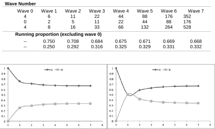
would nominate six more members of group A (75% of the 8 total recruits) and two members of group B (25% of 8). In the next wave of recruitment, those six A’s would recruit nine more A’s (0.75*12) and three B’s, while the two B’s would recruit a total of two A’s and two B’s (each B recruits half A’s and half B’s). If we exclude the seed wave (which is convention in RDS), our revised estimate of the prevalence of group B in the population after two waves of recruitment is 30%. By the seventh wave, our estimated prevalence of B matches the true prevalence to three significant figures (Table 1). While this example started with a seed population composed of only people in group A, we would have reached the estimates of comparable accuracy and efficiency if we had started with only people in group B (Figure 2). Table 1. Over several waves of infection, characteristics in an RDS sample will approach the true
population characteristics.
Wave Number
Wave 0 Wave 1 Wave 2 Wave 3 Wave 4 Wave 5 Wave 6 Wave 7
A 4 6 11 22 44 88 176 352
B 0 2 5 11 22 44 88 176
4 8 16 33 66 132 264 528
Running proportion (excluding wave 0)
A -- 0.750 0.708 0.684 0.675 0.671 0.669 0.668 B -- 0.250 0.292 0.316 0.325 0.329 0.331 0.332
22
This method is subject to a number of assumptions:
(1) The network is completely connected (i.e., we can start from any person and reach any other person on the network within a finite number of steps);
(2) Seeds do not have to be representative of the population, but they should be independently sampled;
(3) We have non-branching recruitment chains;
(4) All ties are reciprocated: this means if X recruited his friend Y, Y would also name X as a friend in the same network;
(5) Degree is accurately reported;
(6) Random referral: people randomly recruit friends in their network (everyone in a person’s network has an equal probability of being recruited);
(7) Samples go through sufficient number of waves to reach equilibrium; and (8) Sampling with replacement.
If all these assumptions hold, RDS can generate unbiased estimates of population characteristics from a non-probability-based sample of seeds. We relaxed assumptions 3 and 8 by using the successive sampling estimator [95], and several other assumptions could be verified in the data. Several additional diagnostic tests were also conducted to assess whether sampling chains reached equilibrium [96].
23 RDS implementation
The 2013 IHBSS round for PWID in Cebu and Mandaue used RDS to recruit PWID in both cities. Seven seeds were identified in each of the two cities to initiate recruitment chains. Peer educators, who were part of the previous Global Fund HIV prevention programs, identified PWID from a range of age groups and geographic areas within each city as
“seeds.” The RDS recruitment system was described to the seeds before the start of data collection, and they were encouraged to bring or inform people they would choose as recruits to go to the study site, to expedite the recruitment process.
A person who presented a coupon was eligible if they had not previously participated in the survey and also fulfilled three other eligibility criteria: (1) they had to be over 15 years old; (2) living in Cebu province; and (3) reported injecting a drug that was not prescribed to them in the last six months.
All eligible participants completed an interview about demographic and behavioral characteristics. This was followed by a blood draw to test for syphilis, Hepatitis C (HCV) and HIV. Participants received 200 Philippine Pesos (PHP, equivalent to just under US$5) as a transportation allowance and were given two coupons, which they were asked to give to friends who were willing to participate in the survey. To further promote recruitment, people were offered a secondary incentive if they were able to successfully recruit new people in the survey. They were offered 50 PHP (just over $1) per successful recruit, with a maximum of 2 recruits per person.
24
(1) How many people (if any) refused the coupon, which revealed how much of his network was saturated (i.e., people who refused because they had already participated, people who refused because they were not interested).
(2) Reciprocation and characterizing his tie with his recruit; in the primary interview, we asked the participant to describe his relationship with his recruiter, so in this interview we asked the question of the recruiter himself, to confirm whether the descriptions of the ties are reciprocated.
(3) Potential social links between his recruiter and his recruit. Because of the anonymous nature of RDS, each person explicitly knows (at most) 3 people in the study: the person who recruited him, and the two people he recruited into the study. But we can ask this person about the ties between his recruiter and recruits, which allows us to identify up to 2 additional ties on the network.
25
Aim 1 Analytic Methods
Estimating population characteristics
To estimate population characteristics, we weighted estimates based on their degree. In its most general form, the RDS-corrected estimate of a population mean of some
characteristic 𝑓 would be:
𝜇̂𝑓 = ∑
𝑓(𝑋𝑖) 𝑑𝑖
𝑛
𝑖=1
∑ 1
𝑑𝑖
𝑛
𝑖=1
⁄
where 𝑑𝑖 refers to each person’s degree, and degree is proportional to one’s probability of
being sampled. This is analogous to a Thompson-Horwitz estimator, used in typical in survey sampling. A number of adjustments or revisions have been added to estimate unbiased RDS-estimates under relaxed assumptions [95,97,98]. We employed one of the most recent of these methods: the successive sampling estimator [95], which did not require assumptions about non-branching chains and sampling with replacement. This method would proceed through an iterative process to converge on unbiased population-level estimates.
RDS Homophily
26
Table 2. Homophily is calculated based on the expected ties under random mixing (left) compared to observed mixing (right).
A B Total A B Total
A 2,670 2,666 5,336 A 3,286 2,050 5,336
B 2,666 2,662 5,328 B 2,050 3,278 5,328
5,336 5,328 10,664 5,336 5,328 10,664
Homophily = (3286 + 3278) / (2670 + 2662) = 1.23
Homophily was calculated as the ratio of the empirical number of in-group ties, compared to the expected number of in-group ties, holding the degree of the two groups constant. In this case, the number of same-group ties (A to A and B to B) was 23% higher than what we expected at random and homophily would be calculated as 1.23. The measure of homophily was centered on 1 (completely random mixing) and represent the proportion of in-group ties more (homophily > 1) or less (homophily < 1) than expected at random.
To estimate homophily from the RDS sample, we used the RDS-weighted degree for each of the groups, to reconstruct a table of in-group and out-group ties expected with random mixing. We then estimated the number of in-group and out-group ties in our population, based on recruitment patterns, weighted by individuals in the network. In this analysis, we considered homophily on variables of where and how people inject.
Measuring the ego-network configuration distribution
The ego-network configuration was used to fit the clustering network parameter in our network. Ego-networks included data on a central person (ego) and all the people directly connected to him (alters) and all the ties among them. The ego-network configurations considered ties among the alters in the ego-network, excluding their ties with the ego.
27
his recruits (i.e., the people to whom he gave RDS coupons). We could not directly ask whether the recruiter (person X) knew his recruit’s recruits (Y and Z). However, the central ego (U) knew that all three of these people were in the survey, and so U can provide
information on whether these alter-alter ties (between X, Y, and Z) exist.
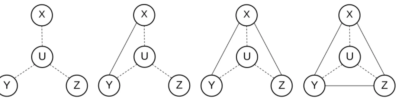
Data on the recruiter-recruit ties (X to Y, X to Z) were collected at the follow-up interview, when individuals returned to receive their secondary incentive. The survey did not explicitly ask if the two recruits knew each other; so data on the Y to Z tie was imputed based on the proportion of dyads that had ties in each city. This meant only three of the four possible ego-network configurations could be observed (first three figures in Figure 3) and the fourth could occur if an additional tie was imputed. We then weighted these
configurations using RDS-weights for each ego in the network.
Figure 3. Ego-network configurations observed from RDS data collected in our survey.
Simulating networks
To estimate the underlying networks in these two cities, we used a method that estimates parameters for an exponential random graph model (ERGM) by simulating
networks and adjusting model parameters that were consistent with the observed networks in our two cities, as demonstrated by Smith [99] and Merli [100]. The method used ERGMs in an iterative process that started from an initial guess of model parameters, which were
X
Z Y
U X
Z Y
U
X
Z Y
U
X
Z Y
28
subsequently adjusted until model fit could not be further improved. The parameters of interest in our model included mixing parameters, which aligned with the homophily in the population; and clustering ties, which we fit to the observed ego-network configurations in our empirical data.
Exponential random graph models
Exponential random graph models (ERGMs) are statistical models that estimate how network properties, such as homophily and transitivity, impact the formation of ties on a network. They follow the form:
Pr(𝑋 = 𝑥) =exp{𝜃
′𝑧(𝑥)}
𝜅(𝜃)
where X is a realization of the network structures, 𝑧(𝑥) refer to the network statistics
(homophily, clustering, etc.), and 𝜅(𝜃) is a normalizing constant, so that probabilities sum to 1 [101-104]. In all but the simplest of cases, the normalizing constant expressed in this equation is too computationally complex to calculate. We avoid estimating this constant by estimating the conditional probability of a single tie, holding the rest of the network constant. Note that if we compare the odds of the presence of a tie vs. the absence of a tie, conditional on the rest of the network, our estimation equation simplifies to:
𝑝(𝑋𝑖𝑗 = 1|𝑋𝑖𝑗𝑐) 𝑝(𝑋𝑖𝑗 = 0|𝑋𝑖𝑗𝑐)
= exp{𝜃′[𝑧(𝑥𝑖𝑗+) − 𝑧(𝑥𝑖𝑗−)]}
29
associations that describe how adolescents choose friends based on a combination of age, gender and race [102]. It has also been used to simulate networks when partial network data were available [99,105].
Fitting the ERGM formula
We seeded these models with two forms of data: (1) an initial network with the joint distribution of characteristics, including degree, of the population; and (2) an initial set of mixing parameters, drawn from the data on observed ties.
Set initial parameters: the initial network
Before we could estimate the network structures, we first estimated characteristics and properties of individuals in the network. We used the RDS weights to estimate the joint distribution of demographic and behavioral characteristics in the populations in each city, and applied this to the estimated PWID population sizes in each (3000 PWID in Cebu, 1500 PWID in Mandaue). The characteristics of interest included: age, categorized into three groups; age at first injection drug use; visits to shooting galleries and tambayan (private injecting parties); frequency of injection, drug of choice, and source for needles and syringes.
30 Initial homophily
Next, we provided ERGM mixing parameters of homophily. In the ERGM formula, these mixing parameters could be interpreted as “the odds that two people of the same group are tied.” We could estimate an analogous logistic regression parameter if we considered the unit of analysis to be a dyad (that is, any pair of two individuals) and the outcome of interest was the presence or absence of a tie. If we collected data on all the observed ties (recruitment ties in the RDS survey) and the homophily among them, compared to a random sample of observed non-ties (a random sample of dyads from the RDS survey), then the resulting logistic regression would estimate the odds of a tie, given the possible characteristics of dyads (A-A, B-B or A-B, for example). The resulting coefficient estimate values were then applied as an initial starting point for the analogous coefficients for mixing, in the ERGM equation.
Initial clustering (GWESP)
Clustering measured the potential of two people having a mutual friend, thus creating a closed triangle on the network. In an ERGM, the clustering parameter could be interpreted as the odds of a tie between two people with the same mutual friend. Unlike measures of homophily, clustering could be estimated in a dyadic logistic regression model, because it is dependent on the presence or absence of other ties on the network, which was the “outcome” of our logistic regression model for homophily. The dependent structure of the clustering coefficient made it quite difficult to estimate because of its vulnerability to model
degeneracy, a consequence of the fact that the closure of one triangle could create many more open triangles. Instead, we parameterized the clustering coefficient by using the
31
𝐺𝑊𝐸𝑆𝑃 = 𝑒𝛼∑{1 − (1 − 𝑒−𝛼)𝑖}𝑝 𝑖 𝑛−2
𝑖=1
where 𝛼 set the rate of decay for each additional partner and 𝑝𝑖 was the number of connected dyads who had individual 𝑖 in common. We initially set our GWESP parameter to 1, and allowed the fitting process to estimate the correct value.
Network estimation process
Using mixing parameters set according to observed homophily and starting the clustering (GWESP) parameter, we then sampled coefficient values within a range (+/- 1) of our original starting point, and then simulated 200 networks for each set of sampled
parameter coefficients. To reduce the sample space of possible networks, we constrained our fits to only those networks with the same degree distribution as the initial random network.
Based on these simulated networks, we extracted the networks that most closely match the ego-network distribution, based on the chi-square statistic. We then reassessed homophily coefficients on those by comparing ties in empirical data (cases) to ties on the simulated networks (controls) to estimate the difference between simulated and observed homophily. These estimates were then used to adjust the corresponding ERGM coefficients to account for this difference. Using these updated ERGM coefficients, we simulated a second set of networks while varying the clustering parameter. We then compared the ego-network distributions on this new set of simulated ego-networks to the empirical distribution, to identify the best-fitting clustering parameter. Updating ERGM parameter for clustering may have changed homophily effects, so these parameters were reassessed and fitted. This process was repeated until we arrived at ERGM formula with the best-fitting ego-network
32
Using this set of 50 networks, we compared network properties, such as homophily statistics, with RDS estimates, to check that the networks we simulated were consistent with the observed data. Consistent networks did not guarantee that our model fully described the true underlying network, but they offered one plausible version of the networks we observed. We then analyzed the properties and characteristics of these simulated networks, in an effort to identify potentially important individuals on the network using centrality measures.
Network Analysis
We analyzed simulated networks to describe the global network characteristics and to identify potentially important individuals within the networks. We looked at several
characteristics relating to the connected components and centrality on the networks, as described below.
Network components
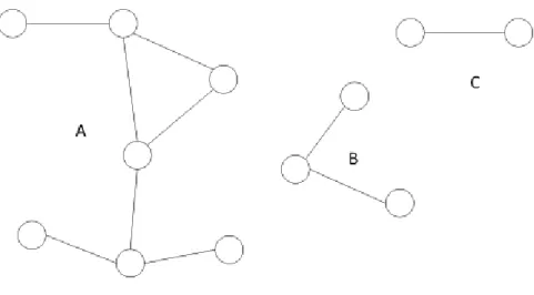
33
Figure 4. Three components make up this network of 12 people; component A is the largest connected component, including 58% (7 out of 12 individuals) of the network.
Geodesic path length and average distance
Within the largest component, we measured the geodesic, or the minimum number of steps it takes for each person to reach every other person on the network [107,108].
Geodesics were measured for every pair of individuals on the same component, so that for a component of size n, we estimated n * (n-1) / 2 paths. People who were not on the same component were an infinite number of steps away, so their geodesic could not be computed. We calculated the average distance, or the average of all geodesics, on the largest component in each of the two cities.
Network centrality
34
Degree: The most basic measure of how much a network influences a person is how many ties a person has, which is called their degree. A person with high degree centrality is well connected and thus has a higher potential for exposure to infection. Increasing degree is therefore highly correlated with higher risk of infection. Similarly, people with higher degree (more connections) can reach a large number of people within a few steps and are also at high risk for onward transmission.
Eigenvector: Degree does not always fully capture centrality. A person with low degree can be connected to one or more persons with very high degree, so that their low degree does not necessarily reflect their reach or connectedness along the network.
Eigenvector centrality captures these higher-order effects of being one or more steps away from very high degree individuals along the network. It is measured as:
𝐶𝐸(𝑛𝑖) =
1
𝜆∑ 𝑎𝑘,𝑖𝑛𝑖
𝑘
where 𝑎𝑘,𝑖 is the adjacency matrix of which nodes are tied; and 𝜆 is a constant.
Closeness: This measure reflects reachability and relative distance between people on the network. A person with high closeness centrality can reach a large number of others in a small number of steps. For an individual person on the network, closeness is measured as the average of the inverse-distance he is from every other person on the network:
𝐶𝑐(𝑛𝑖) = [∑ 𝑑(𝑛𝑖, 𝑛𝑗) 𝑔
𝑗=1
]
−1
where the function d is the distance function, measuring the shortest path between nodes ni
and nj. Individuals with the highest closeness centrality can quickly reach the largest number
35
Betweenness: Individuals with high betweenness centrality lie on many of the shortest paths connecting other people in the network. The measure is a count of the total number of shortest paths an individual lies on.
𝐶𝐵(𝑛𝑖) = ∑ 𝑔𝑗𝑘(𝑛𝑖)/
𝑗<𝑘
𝑔𝑗𝑘
where 𝑔𝑗𝑘 is the number of shortest paths between j and k, and 𝑔𝑗𝑘(𝑛𝑖) is the number of
shortest paths between j and k that go between node ni. Individuals with high betweenness
centrality may be gatekeepers or important bridges between these individuals. However, if there are many paths to between the two individuals, then high betweenness (lying on many of the shortest paths between others) may be of less importance.
Centrality measures tend to be highly correlated, but poor correlation between centrality measures may signal unusual or important structures and particularly unusual individuals on the network. For example, individuals with high betweenness but low degree centrality indicate people who may serve as important bridges between small or large groups of people.
Clustering coefficient
To measure clustering on the network, we use the clustering coefficient, which is a measure of the number of observed triangles on the network as a proportion of the number of possible triangles:
𝜙 = 3 x number of triangles on the network number of connected triples of vertices
36
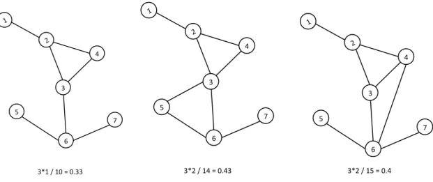
predictable manner with the addition of a tie that will close the triangle, as the closure of one triangle may create a number of new potential triads that were not previously present on the network. In Figure 5, we can add one additional tie to the original component A in two different ways that could result in different measures of the clustering coefficient.
Figure 5. Adding one tie to a network changes the clustering coefficient, but in unpredictable ways.
Clustering can have two consequences for network structure. When clustering is very low, increased clustering can create greater network cohesion, which creates more available paths for infection to travel. Low network cohesion could make the spread of infection may more susceptible to random breaks in transmission that might occur with diseases with low per-contact transmission probabilities [41]. Therefore, some degree of clustering might be needed to ensure the network is sufficiently connected to sustain spread of infection. Beyond a certain level of cohesion, however, added clustering results in the addition of paths that may be redundant because the people they connect are likely to already be infected through other pathways. 1 2 5 3 6 4 7
3*1 / 10 = 0.33
1 2 5 3 6 4 7 1 2 5 3 6 4 7
37
We then considered whether differences in these network characteristics aligned with our expectations, based on the observed differences in the timing and HIV prevalence
patterns in each city.
Aim 1 Limitations
This work employs methods that remain quite new in the area of network estimation and simulation. It may provide potential insights to network structure, but our results are limited in the data we have. Three major limitations were:
(1) Reliability of RDS data: Although respondent-driven sampling is employed widely, there remains some controversy over whether estimates or RDS-weights and uncertainty are accurate [110]. The demographic composition of network simulations, then, were only as reliable as our RDS estimates. Given the difficulty in recruiting this population, however, it was the best available data in this population.
(2) Truncated ego-network distribution: Fitting of the clustering parameter was based on our ego-network distribution. Given the format of our data, our model fit was compared to the distribution of only four possible ego-network configurations, which meant that there could have been a wide range of possible parameters that matched this distribution, and thus we could not guarantee that our coefficient estimates were the singular best solution. (3) Fitting process was limited: The network estimation process was not comprehensive, as
38
Aim 2 Analytic methods
The use of phylogenetic analysis is particularly useful in the study of viral evolution because of the high mutation rate that is unique to viruses. Unlike most organisms in the world, HIV does not have the DNA polymerase and its reverse transcriptase makes multiple base substitutions in every copy of genetic material [111]. We can analyze the genetic material of viruses to identify different generations of the virus to reconstruct a sort of genetic ‘family tree’.
Building the consensus sequences
Each successfully sequenced sample had a large set of 50,000 to 100,000 ‘clean’ reads. To generate the phylogenetic tree, we first had to reduce each set of data to a single consensus sequence that reported the majority nucleotide base (A, C, T, or G) present at each position in the sequence (Table 3). In positions with no clear majority (or a plurality), a placeholder (X) was used to indicate that a base was reported but no clear majority was observed in the data. In the alignment, these were treated as deletions, or missing data. The Center for AIDS Research lab at the University of Hawaii at Manoa used in-house software, Intergroomer (http://courge.ics.hawaii.edu/inte/groomer/), to generate consensus sequences from the data.
Table 3. Building a consensus sequence usually means taking the majority base present at each site.
DATA
1 A A A C T G A G G
2 A A A C T G T G G
3 A A G C T C A G G
4 A A A C T C T G G
5 A A G C T G A G A
39
To properly construct the phylogenetic tree, we first added 286 reference sequences, which we obtained by searching GenBank for all HIV sequences from the Philippines and the 10 closest matches with our sequence data. These data were combined into a single
alignment file.
Sequence alignment
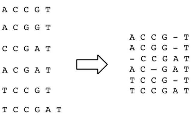
The consensus sequences were aligned with the HXB2-LAV K03455 reference genome using MUSCLE [112,113]. The alignment process was needed to account for errors in the replication process that could result in random insertion or deletion of a base. If we had not properly account for these insertions and deletions, we would overestimate the degree of genetic diversity because some sequences would have been incorrectly shifted by one or two positions (Figure 6). To correct for this, the MUSCLE algorithm iterated through a number of steps to arrive at the best alignment.
Figure 6. Insertion of blank spaces can be necessary to align sequences with each other.
40
initial alignment (MSA1). Using these sequences (with the new insertions), genetic distances were recalculated and another tree was generated, resulting in a second alignment dataset (MSA2). This new alignment (MSA2) was assessed by splitting the new tree into two subtrees. The two subtrees are aligned separately and then rejoined, inserting gaps where needed. The two alignments were scored based on the number and size of gaps added in each sequence; if the score improved, the new alignment was again reassessed. Otherwise, the old alignment was used. Alignments were further confirmed by visual inspection, to ensure that none of the results arose from an unexpected artifact of the data [112,113].
Phylogenetic tree construction
Once our sequences were aligned, we used RAxML to find the best fitting maximum-likelihood phylogenetic tree [114]. The maximum-maximum-likelihood method fitted a model of
evolution and tree topology to the sequence data to estimate the best-fitting tree. Specifically, we maximized the likelihood function such that the tree 𝜏 and evolutionary model M
generated the highest probability of the data, which consisted of base substitutions occurring at site 𝑗 for sequences of length 𝑙 across all sequences in the alignment (𝐷).
𝐿(𝜏, 𝑀, 𝜌|𝐷) = ∏ Pr[𝐷𝑗, 𝜏, 𝑀, 𝜌𝑗 = 1] 𝑙
𝑗=1
We assumed a generalized time-reversible (GTR) evolutionary model, in which nucleotide substitution rates were defined using the Q matrix:
A C G T
𝑄
= (
−𝜇(𝑎𝜋𝐶+ 𝑏𝜋𝐺+ 𝑐𝜋𝑇) 𝑎𝜇𝜋𝐶 𝑏𝜇𝜋𝐺 𝑐𝜇𝜋𝑇
𝑎𝜇𝜋𝐴 −𝜇(𝑎𝜋𝐴+ 𝑑𝜋𝐺+ 𝑒𝜋𝑇) 𝑑𝜇𝜋𝐺 𝑒𝜇𝜋𝑇
𝑏𝜇𝜋𝐴 𝑑𝜇𝜋𝐶 −𝜇(𝑏𝜋𝐴+ 𝑑𝜋𝐶+ 𝑒𝜋𝑇) 𝑓𝜇𝜋𝑇
𝑐𝜇𝜋𝐴 𝑒𝜇𝜋𝐶 𝑓𝜇𝜋𝐺 −𝜇(𝑐𝜋𝐴+ 𝑒𝜋𝐶+ 𝑓𝜋𝐺)
41
In the above matrix, πs represents the observed frequency proportion of base s and
thus sum to 1. The letters a-f are multipliers of the rate of substitution (μ) for each base. We can see the “reversible” aspect of the model in that the rates of change between the different bases are equal, as evidenced by the fact that the letters are symmetric across the diagonal of this matrix. For example, the substitution rate in of A for C (shown in the first column of the second row) is equal to the substitution rate of C for A (second column, first row).
These methods simultaneously estimated the phylogenetic tree and the model
parameters listed above, so they invoked heuristics that allowed us to fit each sequence in the tree so that the tree and model best described the pattern of nucleotide substitutions that we observed. If we had added each sequence in a step-wise manner, we would guarantee reaching a local maximum of the likelihood function. Therefore, we exchanged random branches to rearrange the tree and refitted the model to improve robustness of the model.
To assess branch support or the reliability of our tree branching patterns, we
conducted bootstrapping, in which columns (specific sites) of all the sequences were selected with replacement and then used to construct phylogenetic trees using the
maximum-likelihood process described above. This sampling and estimation process was repeated multiple times. We presented a consensus tree with bootstrap values that represented the proportion of these bootstrapped samples in which each specific branch was observed.
42
No well-defined thresholds exist to determine or identify transmission clusters. Prior work had used somewhat arbitrary values for minimum genetic distance and high bootstrap support [115,116]. Although genetic distance may have been confounded by time as infection continues to evolve within given individuals, this was unlikely in our data, given the very recent emergence of the epidemic in Cebu. In our analysis, we wanted to assess whether we can observe any separation was evident between HIV infections from PWID in Cebu and those in Mandaue.
Aim 2 Limitations
One challenge in the analysis was the low success rate of viral amplification, which resulted in a smaller sample size. Blood and plasma were collected in the Philippines and then separated for HIV, HCV and Syphilis testing before being shipped to the sequencing laboratory at the Hawaii Center for HIV/AIDS (HCFA). In some samples, most of the virus may have degraded, precluding any possibility of amplification or sequencing. Although the amplification success rate of 22% was quite low, there was no indications that degradation was differential with respect to city.
Since the data were collected primarily for public health purposes and not research, the sequencing data were targeted to look in-depth along those regions of the genome that carry clinically important mutations. As a result, the relatively short length of the consensus sequences may not have been sufficient phylogenetic signal to detect underlying differences between two or more different patient sequences.
43
the effects of treatment [111]. While treatment status would be a serious concern in most phylogenetic studies, hospital records (as reported at the central level) indicated that no more than 30 PWID had initiated ART at the time of the 2013 surveillance, so convergent
44
CHAPTER 4: IDENTIFYING NETWORK STRUCTURES THAT IMPACT HIV TRANSMISSION DISEASE DYNAMICS IN THE PHILIPPINES Introduction
While the global HIV response has slowed the epidemic in most of the world, an estimated 2 million new HIV infections occur every year [117]. In the Philippines, only 3500 cases were reported in the first 25 years since the first case was reported in 1984 [118,119]. Since 2008, however, the HIV epidemic has grown at a rapid pace, with the number of reported HIV and AIDS cases increasing by 20-40% each year and over 80% of the 32,000 HIV and AIDS cases reported since 1984 occurring within the last 5 years [119]. In a world where HIV is largely on the decline, the HIV epidemic is just beginning to take hold in the Philippines.
People who inject drugs (PWID) are a highly affected population in the HIV
45
Most new HIV infections among PWID in the Philippines occurred in Cebu, the country’s second largest metropolis. In 2009, HIV surveillance in the metropolis center of Cebu City captured the emergence of an outbreak among people who inject drugs (PWID), where HIV prevalence rose from 0.6% to 53% in the course of one year [11]. Expanded surveillance in neighboring Mandaue City suggested that infection spread more slowly and reached a smaller proportion of the population, even though PWID in both communities exhibited risky injecting practices that would suggest environments ripe for rapid HIV transmission. We investigate whether the network structures that connect PWID within these two cities may explain some of the variation in transmission dynamics observed in the two communities.
Methods
Study population
46
Mandaue cities, and explore whether differences in these structures are associated with differences in the transmission dynamics of HIV in the two cities.
Network parameters of interest
Network structures and characteristics can influence the potential spread of disease in several important ways. We describe both network-level and individual-level characteristics to assess their potential effects on transmission dynamics. At the network level, we identify all network components. A network component is the set of people who can reach each other through network ties. If disease can only be transmitted through these ties, the component defines the potential number of people who could be infected by the introduction of disease on the network or the boundary of infection spread. The size of the largest connected component should help us determine the maximum final size of an epidemic on a network. We measure what proportion of the network is captured in the largest component to define the potential reach, or maximum prevalence of infection. We also estimate average distance, which summarizes the shortest paths (geodesics) between every pair of PWID on the
component. Shorter average distance will accelerate the speed of spread, because we could reach more of the network component in a fewer number of steps. Density of the network is the ties observed on the network, expressed as a proportion of all possible ties. This measure may also impact the connectivity as increasing network density may provide the opportunity shorten paths on the network. We finally measure a clustering coefficient, which is a measure of the proportion of closed triangles on the network. In general, we would expect increases in clustering to create redundant paths on the network and slow transmission [28,39,40].
47
a measure of the number of direct ties or contacts an individual has on the network. Higher average degree on a network should increase the probability of an epidemic occurring [28]. Eigenvector centrality combines higher-order effects of degree (i.e., being connected to someone of high degree will increase eigenvector centrality) and has been associated with risk of infection among PWID [70]. Closeness measures the inverse-path length between an individual and all others on the connected component. Betweenness counts the number of times an individual lies on the shortest path between two other individuals on the network. These centrality measures may identify important individuals or groups of individuals who may influence transmission dynamics across the network.
Data collection methods
48 Statistical analysis and network simulation
Using methods proposed by Smith in 2012 [99] and previously applied to RDS data [100], we estimated coefficient parameters for an exponential random graph model (ERGM), a conditional regression model that relates network characteristics, such as mixing and clustering, with the presence or absence of a network tie [101,103,104].
Our network simulation started from a random network with node characteristics that matched our RDS-weighted population. This random network was combined with an initial set of coefficients for a defined ERGM. A series of new networks were simulated from these coefficients, and their results were adjusted to more closely match the empirical network characteristics of mixing and clustering, as estimated from our RDS-weighted data. The process could be described in four parts. First, we estimated characteristics of individuals on the network and overall network characteristics (mixing and clustering) from the RDS data. Next, we set up the initial ERGM parameters and simulated the networks. Third, we
iteratively adjusted ERGM coefficients and simulate new networks until our coefficient estimates closely resembled the empirical data. We then simulated a number of networks from our final set of coefficients. All analyses were conducted in R statistical software [121], using the RDS [122], igraph [123], and statnet suite [124,125] of packages. We discuss each step in further detail here.
Estimates from RDS data

![Table 4. Demographic and behavioral characteristics of the sample, weighted using Gile’s successive sampling estimator [95]](https://thumb-us.123doks.com/thumbv2/123dok_us/7948380.2112256/67.918.114.798.211.791/table-demographic-behavioral-characteristics-weighted-successive-sampling-estimator.webp)