Vol 7, No 8 (2016)

Available online through

ISSN 2229 – 5046

HOMOTOPY ANALYSIS SOLUTIONS OF MHD FLOW AND HEAT TRANSFER

OF A VISCOELASTIC FLUID FLOW OVER AN EXPONENTIALLY STRETCHING SHEET

EMBEDDED IN A THERMALLY STRATIFIED MEDIUM

P. VIJAYA KUMAR

a*

_{, B. SOUJANYA}

b

a _{Department of Mathematics, GITAM University, Visakhapatnam-530045, India.}

b _{Department of Computer Science Engineering,}

GITAM University, Visakhapatnam-530045, India.

(Received On: 29-07-16; Revised & Accepted On: 23-08-16)

ABSTRACT

MHD boundary layer flow and heat transfer of a viscoelastic fluid over an exponentially stretching sheet embedded in a thermally stratified medium subject to radiation and suction are examined. Using similarity transformation the governing boundary layer non-linear partial differential equations are converted into non-linear ordinary differential equations. Homotopy analysis method (HAM) is applied to get series solution. The convergence of the obtained series solution is discussed explicitly. It is found that the heat transfer rate at the surface increases in presence of thermal stratification. Fluid velocity decreases with increasing magnetic parameter. Fluid velocity decreases with increase of suction parameter. It is noticed that the temperature decreases with increase of suction parameter. Temperature gradient increases considerably with increase of stratification parameter.

Keywords: MHD flow, exponentially stretching sheet, suction, thermally stratified medium, HAM.

INTRODUCTION

In recent years, the study of non-Newtonian fluids has achieved a lot success due to their practical applications in various fields like manufacturing of foods and papers, manufacturing of plastic sheets, etc. The study of boundary layer flow over a continuous solid surface moving with a constant speed was first studied by Sakiadis [1] in 1961. Later Crane [2] extended this problem to a stretching sheet whose surface velocity varies linearly with a certain distancefrom a fixed point. Chang [3] derived a closed form solution of the non-Newtonian flow problem of Rajgoplal et al. [4]. Char [5] discussed the effects of magnetic field and power law surface temperature on heat and mass transfer from a continuous flat surface. Heat and mass transfer characteristics in the presence of transverse magnetic field were obtained by Abel et al. [6]. Raptis [7], Abel and Gousia [8] analysed the viscoelastic fluid flow and heat transfer in the presence of thermal radiation under various physical conditions.

Most of the researchers concentrated on the flow analysis caused by stretching the sheet linearly. Magyari and Keller sheet. Elbashbeshy [10] examined the flow and heat transfer characteristics over an exponentially stretching continuous surface with suction. Bidin and Nazar [11] presented the numerical solutions for the problem of boundary layer flow over an exponentially stretching sheet in the presence of radiation.

The flow due to a heated surface immersed in a stable stratified viscous fluid has been investigated experimentally and analytically by Yang et al. [12]. Recently, Mukhopadhyay [13] analysed the MHD boundary layer flow and heat transfer towards an exponentially stretching sheet embedded in a thermally stratified medium by taking suction into account.

Hence, the aim of the present work is to study the characteristics of MHD boundary layer flow and heat transfer of a viscoelastic fluid over an exponentially stretching sheet embedded in a thermally stratified medium in the presence of suction and radiation using HAM [14, 15].

Corresponding Author: P. Vijaya Kumara*_,

MATHEMATICAL FORMULATION

Consider the flow of an incompressible viscoelastic electrically conducting fluid past a flat heated sheet coinciding with the plane y=0 and the flow being confined toy>0. The flow is generated due to stretching the sheet exponentially by the application of two equal and opposite forces along the x-axis. So that the sheet is stretched keeping the origin fixed. A variable magnetic field of strength

B

is applied in the direction to normal the plate. The sheet is of temperature T_w

( )

x and is embedded in a thermally stratified medium of variable temperature T_∞

( )

x where

( )

x T

( )

x w

T > _∞ . It is assumed that

( )

L x e b T x w

T = ₀+ 2 ,

( )

L

x

e

c

T

x

T

2 0

+

=

∞ where T0 is the reference temperature,

0 0

,

≥

> c

b are constants.

The equations of continuity, momentum, energy and concentration for the flow of viscoelastic fluid are

, 0 = ∂ ∂ + ∂ ∂ y v x u (1) , 2 2 2 2 3 3 2 3 0 2 2 u B y v x u y x u y u y u v y x u u k y u y u v x u u ρ σ ν − ∂ ∂ ∂ ∂ + ∂ ∂ ∂ ∂ ∂ − ∂ ∂ + ∂ ∂ ∂ − ∂ ∂ = ∂ ∂ + ∂ ∂

















(2) , 2 2 y r q y T k y T v x T u p C ∂ ∂ − ∂ ∂ = ∂ ∂ + ∂ ∂













ρ (3)

where u and v are the velocity components in x and y directions,ν _{is the kinematic viscosity,}

k

₀ is the elastic parameter, ρ is the fluid density, σ is the electrical conductivity of the fluid, T is the temperature in the boundary layer, k is the thermal conductivity, q_r is the radiative heat flux.

The boundary conditions are

. y as T T u y at w T T ) x ( V v L x e 0 U w U u ∞ → ∞ → → = = − = = = , 0 , 0 , ,

, ₍₄₎

Here, the subscripts w,∞ refer to the surface and ambient conditions, respectively. U_w is the stretching velocity, U₀ is the reference velocity, L _{is the reference lengt,} V

( )

x >0 is velocity of suction and V

( )

x <0is velocity of blowing,

( )

L

x e V x

V = ₀ 2 , a special type of velocity at the wall is considered. Here

V

₀ is the initial strength of suction.

It is assumed that the variable magnetic field B

( )

x is of the form:

( )

₀

( )

2L,

x e x B x B =

where B₀ is the constant magnetic field.

The equation of continuity is satisfied by the stream functionψ(x,y

)

defined by

,

.

u v y x ψ ψ ∂ ∂ = = − ∂ ∂

Following Rosseland approximation, the radiative heat flux is

, 4 3 4 y T * k * r q ∂ ∂ − = σ

whereσ* is the Stefan-Boltzman constant and k* is the mean absorption coefficient. Further, we assume that the temperature difference within the flow is such that T4is expressed as a linear function of temperature. Hence, expanding T4 in Taylor series about 𝑇𝑇_∞ and neglecting higher order terms, we obtain

.

4 3 3 4 4 ∞ − ∞

≅ T T T

Now, we introduce the following similarity transformations to convert the partial differential equations into ordinary differential equations:

( )

( )

( )

(

)















− ∞ − = + − = = = = , 0 , 2 2 0 , 2 0 2 , , 2 2 0 , 0 T w T T T ) ( ' f f L x e L U v L x e ) ( f U L ) y x ( L x e L U y ' f L x e U u η θ η η η ν η ν ψ ν η η (5)

where η is the similarity variable, f is the dimensionless stream function, θ(η) is a dimensionless temperature of the fluid in the boundary layer region.

Substituting Equation (5) in Equations (2) to (4), we obtain

, 2 2 3 2 1 3 1 2

2f' −ff''= f'''−k f' f'''− ff''''− f''



−M f'











(6)

(

)

0,

3 4

1+



+ − − =











' f St Pr ' f ' f Pr ' '

R θ θ θ (7)

where ν L w U k

k₁ = 0 is the dimensionless viscoelastic parameter,

0 2 0 2 U L B M ρ σ

= is the magnetic parameter,

k * k T * R 3 4 _∞

= σ is the radiation parameter,

k p C Pr ρ ν

= is the Prandtl number, b c

St = is the stratification parameter.

0

>

St implies a stably stratified environment, while St= 0 corresponds to an unstratified environment.

The transformed boundary conditions are

0, ' , 1, 1 0,

' 0, 0, 0 .

f f S at

f as

θ ϕ η

θ ϕ η

= = = = =

= = = → ∞ (8)

where 0

(

or 0

)

2 0

0 _{> <} =

L U

V S

ν is the suction (or blowing) parameter.

HAM Solution

In this section, we employ HAM to solve the equations (6) and (7) subject to the boundary conditions (8). We choose the initial guesses f₀ and θ₀of

f

and θ in the following form

( )

( )

e .

, e

f

η η θ η η − = − − = 0 1 0

The linear operators are selected as

( )

( )

, 2 , 1 θ θ θ = −

− = ' ' L ' f ' ' ' f f L

which have the following properties

(

)

(

)

, , 0 η e 5 C η e 4 C 2 L 0 η e 3 C η e 2 C 1 C 1 L = − + = − + +

where C₁,C₂,C₃,C₄ and C₅ are the arbitrary constants.

(

1− p

)

L₁

(

f

( )

η;p − f₀

( )

η

)

= p₁N₁

[

f

( )

η;p

]

, (9)

(

1− p

)

L₂

(

θ

( )

η;p −θ₀

( )

η

)

= p₂ N₂

[

f

( ) ( )

η;p ,θ η;p

]

, (10) Subject to the boundary conditions

( )

( )

( )

( )

p

( )

p .

p ' f S p ' f p f 0 ; , 1 ; 0 , 0 ; , ; 0 , 0 ; 0 = ∞ = = ∞ = = θ

θ (11)

Based on equations (6) and (7), we define the nonlinear operators

N

₁

and

N

₂ as 2

3 2

( ; ) ( ; ) ( ; )

[ ( ; )] 2 ( ; )

1 3 2

f p f p f p

N f η p η η f η p η

η η η ∂ ∂ ∂ = − + ∂ ∂ ∂













2

3 4 2

( ; ) ( ; ) 1 ( ; ) 3 ( ; ) ( ; )

3 ( ; ) ,

1 3 ₂ 4 ₂ 2

f p f p f p f p f p

k η η f η p η η M η

η η η η η

∂ ∂ ∂ ∂ ∂ − − − − ∂ ∂ ∂ ∂ ∂







_{ }











_{ }





_{ }

(12)

( ) ( )

4 2

( )

;

( ) ( )

;

( ) ( )

;

( )

;

; , ; 1 Pr ; ; Pr ,

2 ₃ 2

p p f p f p

N f η p θ η p R θ η f η p θ η η θ η p S t η

η η η

η ∂ ∂ ∂ ∂ = + + − − ∂ ∂ ∂ ∂















_{ }

_

_

_

_

_



_{ }

_









(13)

When p=0 and p=1, we obtain

( )

( )

( ) ( )

( )

;0 ₀

( )

( ) ( )

;1 . , 1 ; 0 0 ; η θ η θ η θ η θ η η η η = = =

= f f f

f

(14)

Thus, as

p

increases from 0 to 1 then f

( )

η;p andθ

( )

η;p vary from initial approximations to the exact solutions of the original nonlinear differential equations.

Now, expanding

f

( )

η

;

p

and

θ

( )

η

;

p

in Taylor’s series w.r.to

p

, we have

(

;

)

( )

( )

, 1 0 m m m p f f p

f η η

∑

η

∞ =

+

= (15)

(

;

)

( )

( )

, 1 0 m m m p

p θ η θ η

η

θ

∑

∞

= +

= (16)

where

( )

(

)

0

;

1

,

!

m m m p

f

p

f

m

p

η

η

=

∂

=

∂

( )

(

)

0

;

1

.

!

m m m p

p

m

p

θ η

θ η

=

∂

=

∂

(17)

( )

( )

( )

,

1 0

m p m fm f

p ;

f

η η ∑∞ η

= +

= (15)

( )

( )

( )

, 1 0 m p m m p

; θ η θ η

η

θ ∑∞

= +

= (16)

where

( )

1

( )

; ,

! ₀

m f p

fm m

m p _p

η

η = ∂

∂ ₌

( )

1

( )

; . ! 0 m p m m m p p θ η

θ η = ∂

∂ ₌ (17)

If the initial approximations, auxiliary linear operators and non-zero auxiliary parameters are chosen in such a way that the series (15) to (16) are convergent at p =1, then

( )

( )

( )

,

1

0 η η

η ∑∞

= + =

m fm f

f (18)

( )

( )

( )

.

0

1 m m

θ η =θ η + ∑∞ θ η =

Differentiating Equations (9) and (10) m times w.r.to

p

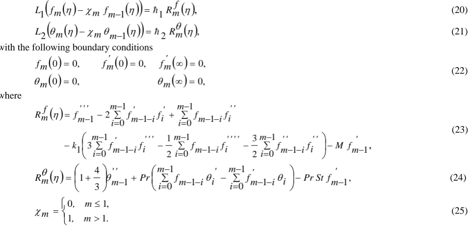
, setting p=0, and finally dividing with m!, we get the mth-order deformation equations as follows

( )

( )

(

₁

)

₁

( )

,

1 η χ η η

f m R m f m m f

L − ₋ = (20)

( )

( )

(

₁

)

₂

( )

,

2 η θ η θ χ η

θ_{m m m} R_m

L − ₋ = (21)

with the following boundary conditions

( )

( )

( )

( )

0 0,

( )

0,

, 0 , 0 0 , 0 0 = ∞ = = ∞ = = m m ' m f ' m f m f θ

θ (22) where

( )

,

1 1 0 1 2 3 1 0 1 2 1 1 0 1 3 1 1 0 1 1 0 1 2 1 ' m f M ' ' i f m i ' ' i m f ' ' ' ' i f m

i fm i ' ' ' i f m i ' i m f k ' ' i f m

i fm i ' i f m i ' i m f ' ' ' m f f m R − − ∑− = −− − ∑− = −− − ∑− = − − − ∑− = −− + ∑− = − − − − =













η (23)

( )

1 ₁,

0 1 1 0 1 1 3 4

1 m _i PrSt f_m'

i ' i m f m i ' i i m f Pr ' ' m m

R ∑− − ₋

= − − − ∑− = −− + − + =

_























_{θ θ θ}

η θ (24)







> ≤ = . m , m ,

m _{1 1}

, 1 0

χ (25)

If we let

f

_m*

(

η

),

θ

_m*

(

η

)

and

φ

_m*

(

η

)

as the special solutions of mth order deformation equations, then the general solution is given by

*

( ) ( ) _{1 2 3} ,

*

( ) ( ) _{4 5} ,

f_m f_m C C e C e

C e C e

m m

η η

η η

η η

θ η θ η

−

= + + +

−

= + + (26)

where the integral constants C_i(i =1to 5) are determined using the boundary conditions.

Convergence of HAM solution

The convergence region and rate of approximation of series solutions obtained using HAM are mainly dependent on the non-zero auxiliary parameters ₁and ₂. In order to find the appropriate values of ₁ and ₂, -curves are

plotted in Fig. 1. From the figure, it is clear that the valid regions of ₁ and ₂are about [-1.0, 0.0]. Our computations indicate that the series converge in the whole region of η when ₁ =₂ = −0.75

.

The convergence of homotopy solution for different orders of approximations is given in Table 1.

Figure 1: -curves of f''(0) andθ'(0) for 20th order approximation when . . S . St . Pr . R . M .

k₁=01, =05, =05, =071, =02, =01

-1.5 -1 -0.5 0 0.5

-10 -5 0 5 10 15 h

1, h2

f ′′ (0 ), θ′ (0 )

f′′(0)

Table 1: Convergence of HAM solution for different orders of approximations when .

. S . St . Pr . R . M .

k₁=01, =05, =05, =071, =02, =01 Order

−

f

'

'

(

0

)

−

θ

'

(

0

)

5 1.644127 0.484227 10 1.645532 0.461557 15 1.645720 0.451515 20 1.645701 0.450992 25 1.645705 0.450961 30 1.646704 0.450954 35 1.646704 0.450961 40 1.646704 0.450954 45 1.646704 0.450951 50 1.646704 0.450951

RESULTS AND DISCUSSION

To ensure the accuracy of the applied method, the values of heat transfer rate

−

θ

'

(

0

)

are compared with the available results in the literature and are presented in Table 2.

Table 2: Comparison of −θ'(0) for different values of M, R, Pr when k₁=St =S=0.0.

M

R

Pr

Bidin and Nazar [11] Seini and Makinde [16] HAM

0.0 0.0 1.0 0.9547 0.954811 0.954783

0.0 0.0 3.0 1.8691 1.869069 1.869067

0.0 1.0 1.0 0.5315 -- 0.531503

1.0 0.0 1.0 0.8611 0.861509 0.861427

0.0 1.0 1.0 -- -- 0.334521

1.0 0.1 2.14 -- -0.268846 -0.268849

In the present study, the following default parameter values are adopted for computations: .

. S . St . Pr . R . M .

k₁=01, =05, =05, =071, =02, =01

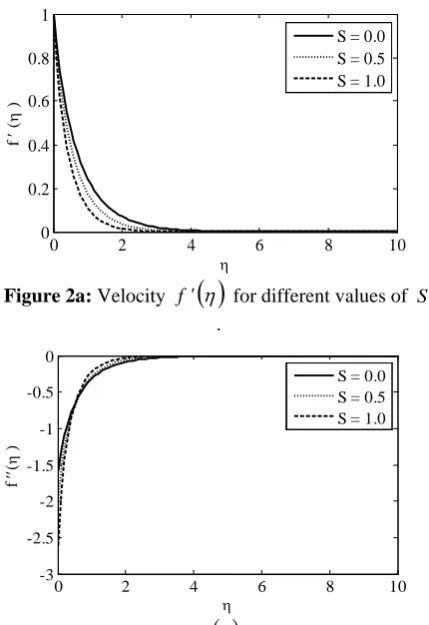
Figure 2a: Velocity f'

( )

η for different values of S .

Figure 2b: Shear stress f''

( )

η for different values of S.

0 2 4 6 8 10

0 0.2 0.4 0.6 0.8 1

η

f

′

(

η

)

S = 0.0 S = 0.5 S = 1.0

0 2 4 6 8 10

-3 -2.5 -2 -1.5 -1 -0.5 0

η

f

′′

(

η

)

Figures 2a and 2b illustrates the effects of suction parameter S on velocity and shear stress profiles, respectively, for exponentially stretching sheet. From figure 2a it is observed that velocity decreases significantly with increasing suction parameter. From Figure 2b, it is very clear that the shear stress decreases initially with the suction parameter S, but shear stress increases significantly after a certain distance η from the sheet. It is observed that, when the wall

suction

(

S >0

)

is considered, this causes a decrease in the boundary layer thickness and the velocity field is reduced.

Figure 2c: Temperature θ

( )

η for different values of S.

Figure 2d: Temperature gradient θ'

( )

η for different values of S.

Figures 2c and 2d represent the temperature and temperature gradient profiles for variable suction parameter S. From figure 2c it is seen that temperature decreases with increasing suction parameter. The temperature gradient decreases initially with the suction parameter S, but it increases after a certain distance η from the sheet. Far away from the wall, such feature is smeared out Figure 2d. Thus, suction at the surface has a tendency to reduce both the hydrodynamic and thermal boundary layer thicknesses.

Figure 3a: Velocity f'

( )

η _{for different values of 1}k .

0 2 4 6 8 10

0 0.2 0.4 0.6 0.8

η

θ

(

η

)

S = 0.0 S = 0.5 S = 1.0

0 2 4 6 8 10

-0.8 -0.6 -0.4 -0.2 0

η

θ

′

(

η

)

S = 0.0 S = 0.5 S = 1.0

0 2 4 6 8 10

0 0.2 0.4 0.6 0.8 1

η

f

′

(

η

)

k₁ = 0.0

k₁ = 0.2

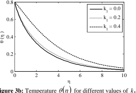
Figure 3b: Temperature θ

( )

η _{for different values of 1}k .

The effect of viscoelastic parameter on velocity and temperature is shown in Figures 3a and 3b. As shown in the figures velocity is decreasing while temperature is increasing with the increase of 1k . This is due to the tensile stress introduced by viscoelasticity which causes transverse contraction of the boundary layer.

Figures 4a and 4b illustrate the influence of magnetic parameter on velocity and temperature profiles. As M increases, the Lorentz force which has the tendency to slow down the motion of the fluid also increases. Hence, the velocity of the fluid decreases whereas temperature increases.

Figure 4a: Horizontal velocity f'

( )

η for different values of M.

Figure 4b: Temperature θ

( )

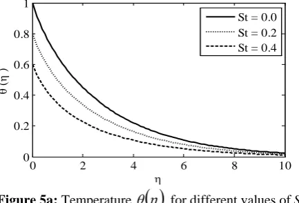
η for different values of M.

Figure 5a is the graphical representation of temperature profiles θ

( )

η for several values of stratification parameter St. It is found that the temperature decreases as the stratification parameter St increases.

The temperature gradient increases with an increase in stratification parameter St as shown in the figure 5b.

0 2 4 6 8 10

0 0.2 0.4 0.6 0.8

η

θ

(

η

)

k

1 = 0.0

k

1 = 0.2

k

1 = 0.4

0 2 4 6 8 10

0 0.2 0.4 0.6 0.8 1

η

f

′

(

η

)

M = 0.0 M = 0.5 M = 1.0

0 2 4 6 8 10

0 0.2 0.4 0.6 0.8

η

θ

(

η

)

Figure 5a: Temperature θ

( )

η for different values ofSt.

In case of higher Prandtl values the diffusion of heat away from the heated surface is very slow when compared to the smaller Prandtl values. Hence temperature decreases with the increase Prandtl number as shown in the figure 6.

Figure 5b: Temperature gradient

θ

'

( )

η

for different values of

St

.

Figure 6: Temperature θ

( )

η for different values ofPr.

Figure 7: Temperature θ

( )

η for different values ofR.

0 2 4 6 8 10

0 0.2 0.4 0.6 0.8 1

η

θ

(

η

)

St = 0.0 St = 0.2 St = 0.4

0 2 4 6 8 10

-0.5 -0.4 -0.3 -0.2 -0.1 0

η

θ

′

(

η

)

St = 0.0 St = 0.2 St = 0.4

0 2 4 6 8 10

0 0.2 0.4 0.6 0.8

η

θ

(

η

)

Pr = 0.1 Pr=0.71 Pr=1.0

0 2 4 6 8 10

0 0.2 0.4 0.6 0.8

η

θ

(

η

)

The effect of radiation parameter R on temperature is displayed in Fig. 9. It is noticed that the temperature increases with the increase ofR. This is due to the fact that the thermal boundary layer thickness increases with the increase of radiation parameter.

CONCLUSIONS

In the present analysis MHD boundary layer flow and heat transfer towards an exponentially stretching sheet embedded in a thermally stratified medium subject to suction and radiation are described. The effect of suction as well as magnetic parameter on a viscoelastic incompressible fluid is to suppress the velocity field which in turn causes the enhancement of the skin-friction coefficient. Rate of transport is reduced with the increasing magnetic field. The temperature decreases with increasing values of the stratification parameter.

REFERENCES

1. Sakiadis B. S., Boundary-layer behaviour on continuous solid surfaces, American Institute of Chemical Engineers, 7(1961), 26-28.

2. Crane L. J., flow past a stretching sheet, Zeitschrift für angewandte Mathematik und Physik, 21(1970), 645-647.

3. Chang W. D., The non uniqueness of the flow of a viscoelastic fluid over a stretching sheet, Quarterly journal of Applied Mathematics, 47(1989), 365-366.

4. Rajagopal K. R., Na T. Y. and Gupta A. S., Flow of a viscoelastic fluid over a stretching sheet, Rheologica Acta, 23(1984), 213-215.

5. Char M. I., Heat and mass transfer in a hydromagnetic flow of the viscoelastic fluid over a stretching sheet, Journal of Mathematical Analysis and Applications, 186(1994), 674-689.

6. Abel S., Veena P. H., Rajagopal K. and Pravin V. K., Non-Newtonian magnetohydrodynamic flow over a stretching surface with heat and mass transfer, International Journal of Non-Linear Mechanics, 39(2004), 1067-1078.

7. Raptis A., Technical note: Flow of a micro polar fluid past a continuously moving plate by the presence of radiation, International journal of Heat Mass Transfer, 41(1998), 2865–2866.

8. Abel M. S. and Gousia Begum, Heat transfer in MHD viscoelastic fluid flow on stretching sheet with heat source/sink, viscous dissipation, stress work and radiation for the case of large Prandtl number, Chemical Engineering Communications, 195(2008), 1503-1523.

9. Magyari E. and Keller B., Heat and mass transfer in the boundary layers on an exponentially stretching continuous surface, Journal of Physics D: Applied Physics, 32(1999), 577-585.

10. Elbashbeshy E. M. A., Heat transfer over an exponentially stretching continuous surface with suction, Archives of Mechanics, 53(2001), 643-651.

11. Bidin B. and Nazar R., Numerical solution of the boundary layer flow over an exponentially stretching sheet

with thermal radiation, European Journal of Scientific Research, 33(2009), 710-717.

12. Yang K.T., Novotny J. L. and Cheng Y.S., Laminar free convection from a non-isothermal plate immersed in a temperature stratified medium, International Journal of Heat and Mass Transfer, 15(1972),1097–1109. 13. Swati Mukhopadhyay, MHD boundary layer flow and heat transfer over an exponentially stretching sheet

embedded in a thermally stratified medium, Alexandria Engineering Journal, 52(2013), 259-265.

14. Liao S. J., The proposed homotopy analysis technique for the solution of non-linear problems [Ph.D. thesis], Shanghai Jiao Tong University, 1992.

15. Hayat T. and Sajid M., Analytic solution for axisymmetric flow and heat transfer of a second grade fluid past a stretching sheet, International Journal of Heat and Mass Transfer, 50(2007), 75-84.

16. Seini Y. I. and Makinde O. D., MHD boundary layer flow due to exponential stretching surface with radiation and chemical reaction, Mathematical Problems in Engineering, 2013, 1-7.

Source of support: Nil, Conflict of interest: None Declared