*** AdS-Fermi-finalrevised-new2.tex ***
Constructing the AdS dual of a Fermi liquid:
AdS Black holes with Dirac hair
Mihailo ˇCubrovi´c, Jan Zaanen, Koenraad Schalm
1 Institute Lorentz for Theoretical Physics, Leiden University
P.O. Box 9506, Leiden 2300RA, The Netherlands
Abstract
We provide new evidence that the holographic dual to a strongly coupled charged Fermi liquid has a non-zero fermion density in the bulk. We show that the pole-strength of the stable quasiparticle characterizing the Fermi surface is encoded in the spatially averaged AdS probability density of a single normalizable fermion wavefunction in AdS. Recalling Migdal’s theorem which relates the pole strength to the Fermi-Dirac characteristic discontinuity in the number density at ωF, we conclude that the AdS dual of a Fermi liquid is described by occupied on-shell fermionic modes in AdS. Encoding the occupied levels in the total probability density of the fermion field directly, we show that an AdS Reissner-Nordstr¨om black hole in a theory with charged fermions has a critical temperature, at which the system undergoes a first-order transition to a black hole with a non-vanishing profile for the bulk fermion field. Thermodynamics and spectral analysis confirm that the solution with non-zero AdS fermion-profile is the preferred ground state at low temperatures.
Email addresses: cubrovic, jan, kschalm@lorentz.leidenuniv.nl.
1
Introduction
Fermionic quantum criticality is thought to be an essential ingredient in the full theory of high Tc
superconductivity [1, 2]. The cleanest experimental examples of quantum criticality occur in heavy-fermion systems rather than highTccuprates, but the experimental measurements in heavy fermions
raise equally confounding theoretical puzzles [3]. Most tellingly, the resistivity scales linearly with the temperature from the onset of superconductivity up to the crystal melting temperature [4] and this linear scaling is in conflict with single correlation length scaling at criticality [5]. The failure of standard perturbative theoretical methods to describe such behavior is thought to indicate that the underlying quantum critical system is strongly coupled [6, 7].
The combination of strong coupling and scale-invariant critical dynamics makes these systems an ideal arena for the application of the AdS/CFT correspondence: the well-established relation between strongly coupled conformal field theories (CFT) and gravitational theories in anti-de Sitter (AdS) spacetimes. An AdS/CFT computation of single-fermion spectral functions — which are directly experimentally accessible via Angle-Resolved Photoemission Spectroscopy [8, 9, 10] — bears out this promise of addressing fermionic quantum criticality [11, 12, 13, 14] (see also [15, 16]). The AdS/CFT single fermion spectral function exhibits distinct sharp quasiparticle peaks, associated with the formation of a Fermi surface, emerging from a scale-free state. The fermion liquid which this Fermi surface captures is generically singular: it has either a non-linear dispersion or non-quadratic pole strength [11, 13]. The precise details depend on the parameters of the AdS model.
From the AdS gravity perspective, peaks with linear dispersion correspond to the existence of a stable charged fermionic quasinormal mode in the spectrum of a charged AdS black hole. The existence of a stable charged bosonic quasinormal mode is known to signal the onset of an instability towards a new ground state with a pervading Bose condensate extending from the charged black hole horizon to the boundary of AdS. The dual CFT description of this charged condensate is spontaneous symmetry breaking as in a superfluid and a conventional superconductor [17, 18, 19, 20]. For fermionic systems empirically the equivalent robust T = 0 groundstate is the Landau Fermi Liquid — the quantum groundstate of a system with a finite number of fermions. The existence of a stable fermionic quasinormal mode suggests that an AdS dual of a finite fermion density state exists.
We construct here the AdS/CFT rules for CFTs with a finite fermion density. The essential ingredient will be the Migdal’s theorem, which relates the characteristic jump in fermion occupation number at the energy ωF of the highest occupied state to the pole strength of the quasiparticle.
The latter we know from the spectral function analysis and its AdS formulation is therefore known. Using this, we show that the fermion number discontinuity is encoded in the probability densityof the normalizable wavefunction of the dual AdS fermion field.
These AdS/CFT rules prove that the AdS dual of a Fermi liquid is given by a system with occupied fermionic states in the bulk. The Fermi liquid is clearly not a scale invariant state, but any such states will have energy, momentum/pressure and charge and will change the interior geometry from AdS to something else. Which particular (set of) state(s) is the right one, it does not yet tell us, as this conclusion relies only on the asymptotic behavior of fermion fields near the AdS boundary. Here we shall take the simplest such state: a single fermion.1 Constructing the
associated backreacted asymptotically AdS solution, we find that it is already good enough to solve several problems of principle:
• Fermionic quantum critical systems should undergo a phase transition to a Fermi liquid at low temperatures, except when one is directly above the QCP. Likewise we find that the dual of the quantum critical state, a charged AdS black hole in the presence of charged fermionic modes, has a critical temperature below which fermionic Dirac “hair” forms. The derivative of the free energy has the characteristic discontinuity of a first order transition. This has to be the case: A fermionic quasinormal mode can never cause a linear instability indicative of a continuous phase transition. In the language of spectral functions, the pole of the retarded Green’s function can never cross to the upper-half plane [13].2 The absence of a perturbative instability between this conjectured Dirac ”black hole hair” solution and the “bald” charged AdS black hole can be explained if the transition is a first order gas-liquid transition. The existence of first order transition follows from a thermodynamic analysis of the free energy rather than a spectral analysis of small fluctuations.
• This solution with finite fermion number is the preferred ground state at low temperatures. The bare charged AdS black hole in a theory with charged fermions is therefore a false vacuum. Confusing a false vacuum with the true ground state can lead to anomalous results. Indeed the finite temperature behavior of fermion spectral functions in AdS Reissner-Nordstr¨om, exhibited in the combination of the results of [11, 13] and [12], shows strange behavior. The former [11, 13] found sharp quasiparticle peaks at a frequency ωF = 0 in natural AdS units,
whereas the latter [12] found sharp quasiparticle peaks at finite Fermi energy ωF 6= 0. As
we will show, both peaks in fact describe the same physics: the ωF 6= 0 peak is a finite temperature manifestation of (one of the) ω = 0 peaks in [13]. Its shift in location at finite temperature is explained by the existence of the nearby true finite fermion density ground state, separated by a potential barrier from the AdS Reissner-Nordstr¨om solution.
• The charged AdS-black hole solution corresponds to a CFT system in a state with large ground state entropy. This is the area of the extremal black-hole horizon atT = 0. Systems with large ground-state entropy are notoriously unstable to collapse to a low-entropy state, usually by spontaneous symmetry breaking. In a fermionic system it should be the collapse to the Fermi liquid. The final state will generically be a geometry that asymptotes to Lifschitz type, i.e. the background breaks Lorentz-invariance and has a double-pole horizon with vanishing area, as expounded in [25]. Although the solution we construct here only considers the backreaction on the electrostatic potential, we show that the gravitational energy density diverges at the horizon in a similar way as other systems that are known to gravitationally backreact to a Lifshitz solution. The fully backreacted geometry includes important separate physical aspects — it is relevant to the stability of the Fermi liquid — and will be considered in a companion article.
The Dirac hair solution thus captures the physics one expects of the dual of a Fermi liquid. We have based its construction on a derived set of AdS/CFT rules to describe systems at finite fermion density. Qualitatively the result is as expected: that one also needs occupied fermionic states in the bulk. Knowing this, another simple candidate is the dual of the backreacted AdS-Fermi-gas [25]/electron star [26] which appeared during the course of this work.3 The difference between the
two approaches are the assumptions used to reduce the interacting Fermi system to a tractable solution. As explained in the recent article [30], the Fermi-gas and the single Dirac field are the
2Ref. [39] argues that the instability can be second order.
two “local” approximations to the generic non-local multiple fermion system in the bulk, in very different regimes of applicability. The electron-star/Fermi-gas is considered in the Thomas-Fermi limit where the microscopic charge of the constituent fermions is sent to zero keeping the overall charge fixed, whereas the single Dirac field clearly is the ’limit’ where the microscopic charge equals the total charge in the system. This is directly evident in the spectral functions of both systems. The results presented here show that each pole in the CFT spectral function corresponds to a unique occupied Fermi state in the bulk; the electron star spectra show a parametrically large number of poles [31, 32, 30], whereas the Dirac hair state has a single quasiparticle pole by construction. The AdS-Dirac-hair black hole derived here therefore has the benefit of a direct connection with a unique Fermi liquid state in the CFT. This is in fact the starting point of our derivation.
In the larger context, the existence of both the Dirac hair and backreacted Fermi gas solution is not a surprise. It is a manifestation of universal physics in the presence of charged AdS black holes. The results here, and those of [11, 13, 25, 26], together with the by now extensive literature on holographic superconductors, i.e. Bose condensates, show that at sufficiently low temperature in units of the black-hole charge, the electric field stretching to AdS-infinity causes a spontaneous discharge of the bulk vacuum outside of the horizon into the charged fields of the theory — whatever their nature. The positively charged excitations are repelled by the black hole, but cannot escape to infinity in AdS and they form a charge cloud hovering over the horizon. The negatively charged excitations fall into the black-hole and neutralize the charge, until one is left with an uncharged black hole with a condensate at finiteT or a pure asymptotically AdS condensate solution atT = 0. As [25, 26] and we show, the statistics of the charged particle do not matter for this condensate formation, except in the way it forms: bosons superradiate and fermions nucleate. The dual CFT perspective of this process is “entropy collapse”. The final state therefore has negligible ground state entropy and is stable. The study of charged black holes in AdS/CFT is therefore a novel way to understand the stability of charged interacting matter which holds much promise.
2
From Green’s function to AdS/CFT rules for a Fermi Liquid
We wish to show how a solution with finite fermion number — a Fermi liquid — is encoded in AdS. The exact connection and derivation will require a review of what we have learned of Dirac field dynamics in AdS/CFT through Green’s functions analysis. The defining signature of a Fermi liquid is a quasi-particle pole in the (retarded) fermion propagator,
GR=
Z
ω−µR−vF(k−kF)
+ regular (2.1)
Phenomenologically, a non-zero residue at the pole, Z, also known as the pole strength, is the indicator of a Fermi liquid state. Migdal famously related the pole strength to the occupation number discontinuity at the pole (ω= 0):
Z = lim
→0[nF(ω−)−nF(ω+)] (2.2)
where
nF(ω) =
Z
d2kfF D
ω
T
ImGR(ω, k).
where fF D is the Fermi-Dirac distribution function. Vice versa, a Fermi liquid with a Fermi-Dirac
Using our knowledge of fermionic spectral functions in AdS/CFT we shall first relate the pole-strength Z to known AdS quantities. Then, using Migdal’s relation, the dual of a Fermi liquid is characterized by an asymptotically AdS solution with non-zero value for these very objects.
The Green’s functions derived in AdS/CFT are those of charged fermionic operators with scaling dimension ∆, dual to an AdS Dirac field with mass m = ∆− d
2. We shall focus on d = 2 + 1
dimensional CFTs. In its gravitational description, this Dirac field is minimally coupled to 3 + 1 dimensional gravity and electromagnetism with the action
S = Z
d4x√−g
1 2κ2
R+ 6
L2
− 1
4F
2
M N−Ψ(¯ D/ +m)Ψ
. (2.3)
For zero background fermions, Ψ = 0, a spherically symmetric solution is a charged AdS4 black-hole
background
ds2 = L
2α2
z2 −f(z)dt
2+dx2+dy2 +L
2
z2
dz2
f(z) ,
f(z) = (1−z)(1 +z+z2−q2z3),
A(0bg) = 2qα(z−1) . (2.4)
HereA(0bg) is the time-component of theU(1)-vector-potential, Lis the AdS radius and the temper-ature and chemical potential of the black hole equal
T = α
4π(3−q
2) , µ
0 =−2qα, (2.5)
where q is the black hole charge.
To compute the Green’s functions we need to solve the Dirac equation in the background of this charged black hole:
eMAΓA(DM +iegAM)Ψ +mΨ = 0 , (2.6)
where the vielbeineM
A, covariant derivative DM and connectionAM correspond to the fixed charged
AdS black-hole metric and electrostatic potential (2.4) andgis the fermion charge. DenotingA0 = Φ
and taking the standard AdS-fermion projection onto Ψ± = 12(1±ΓZ)Ψ, the Dirac equation reduces
to
(∂z+A±) Ψ± = ∓T/Ψ∓ (2.7)
with
A± = −
1 2z
3− zf
0
2f
± mL
z√f ,
/
T = i(−ω+gΦ)
αf γ
0+ i
α√fkiγ
i . (2.8)
Here γµ are the 2+1-dimensional Dirac matrices, obtained after decomposing the 3+1 dimensional Γµ-matrices.
Explicitly the Green’s function is extracted from the behavior of the solution to the Dirac equation at the AdS-boundary. The boundary behavior of the bulk fermions is
Ψ+(ω, k;z) = A+z
3
2−m+B
+z
5
2+m+. . . ,
Ψ−(ω, k;z) = A−z
5
2−m+B−z 3
whereA±(ω, k), B±(ω, k) are not all independent but related by the Dirac equation at the boundary
A− =−
iµ
(2m−1)γ
0A
+ , B+ =−
iµ
(2m+ 1)γ
0B
− . (2.10)
The CFT Green’s function then equals [12, 33, 11]
GR= lim z→0z
−2mΨ−(z)
Ψ+(z)
−singular = B−
A+
. (2.11)
In other words, B− is the CFT response to the (infinitesimal) source A+. Since in the Green’s
function the fermion is a fluctuation, the functions Ψ±(z) are now probe solutions to the Dirac
equation in a fixed gravitational and electrostatic background (for ease of presentation we are considering Ψ±(z) as numbers instead of two-component vectors). The boundary conditions at
the horizon/AdS interior determine which Green’s function one considers, e.g. infalling horizon boundary conditions yield the retarded Green’s function. For non-zero chemical potential this fermionic Green’s function can have a pole signalling the presence of a Fermi surface. This pole occurs precisely for a (quasi-)normalizable mode, i.e. a specific energyωF and momentumkF where
the external source A+(ω, k) vanishes (for infalling boundary conditions at the horizon).
Knowing that the energy of the quasinormal mode is alwaysωF = 0 [11] and following [13], we expand GR around ω= 0 as:
GR(ω) =
B(0)+ωB(1)+. . .
A(0)+ +ωA(1)+ +. . .. (2.12)
A crucial point is that in this expansion we are assuming that the pole will correspond to a stable quasiparticle, i.e. there are no fractional powers of ω less than unity in the expansion around
ωF = 0 [13]. Fermions in AdS/CFT are of course famous for allowing more general pole-structures
corresponding to Fermi-surfaces without stable quasiparticles [13], but those Green’s functions are not of the type (2.1) and we shall therefore not consider them here. The specific Fermi momentum
kF associated with the Fermi surface is the momentum value for which the firstω-independent term
in the denominator vanishes A(0)+ (kF) = 0 — for this value of k =kF the presence of a pole in the
Green’s functions at ω = 0 is manifest. Writing A(0)+ = a+(k−kF) +. . . and comparing with the
standard quasi-particle propagator,
GR= Z
ω−µR−vF(k−kF)
+ regular (2.13)
we read off that the pole-strength equals
Z =B−(0)(kF)/A
(1) + (kF).
We thus see that a non-zero pole-strength is ensured by a non-zero value of B−(ω= 0, k=kF)
— the “response” without corresponding source as A(0)(k
F) ≡ 0. Quantatively the pole-strength
also depends on the value of A(1)+ (kF)≡ ∂ωA+(kF)|ω=0, which is always finite. This is not a truly
independent parameter, however. The size of the pole-strength has only a relative meaning w.r.t. to the integrated spectral density. This normalization of the pole strength is a global parameter rather than an AdS boundary issue. We now show this by proving that A(1)+ (kF) is inversely proportional
to B−(0)(kF) and hence Z is completely set by B
(0)
− (kF), i.e. Z ∼ |B
(0)
f
W(Ψ+,A,Ψ+,B) of the Wronskian W(Ψ+,A,Ψ+,B) = Ψ+,A∂zΨ+,B −(∂zΨ+,A)Ψ+,B for two solutions
to the second order equivalent of the Dirac equation for the field Ψ+
∂z2+P(z)∂z+Q+(z)
Ψ+ = 0 (2.14)
that is conserved (detailed expressions for P(z) and Q+(z) are given in eq. (2.21)):
f
W(Ψ+,A(z),Ψ+,B(z), z;z0) = exp Z z
z0 P(z)
W(Ψ+,A(z),Ψ+,B(z)) , ∂zfW = 0. (2.15)
Here z0−1 is the infinitesimal distance away from the boundary at z = 0 which is equivalent to the U V-cutoff in the CFT. Setting k = kF and choosing for Ψ+,A = A+z3/2−m
P∞
n=0anzn and
Ψ+,B =B+z5/2+mP
∞
n=0bnz
nr the real solutions which asymptote to solutions with B
+(ω, kF) = 0
and A+(ω, kF) = 0 respectively, but for a value of ω infinitesimally away from ωF = 0, we can
evaluate Wf at the boundary to find,4
f
W =z03(1 + 2m)A+B+ =µz03A+B− (2.16)
The last step follows from the constraint (2.10) where the reduction from two-component spinors to functions means that γ0 is replaced by one of its eigenvalues ±i. Taking the derivative of
f
W at
ω = 0 fork =kF and expandingA+(ω, kF) andB−(ω, kF) as in (2.12), we can solve for A
(1)
+ (kF) in
terms of B−(0)(kF) and arrive at the expression for the pole strength Z in terms of|B
(0)
− (kF)|2:
Z = µz
3 0
∂ωWf|ω=0,k=kF
|B(0)− (kF)|2 . (2.17)
Because∂ωfW, asfW, is a number that is independent ofz, this expression emphasizes that it is truly the nonvanishing subleading term B−(0)(ωF, kF) which sets the pole strength, up to a normalization ∂ωfW which is set by the fully integrated spectral density. This integration is always UV-cut-off dependent and the explicit z0 dependence should therefore not surprise us.5 We should note
that, unlike perturbative Fermi liquid theory, Z is a dimensionful quantity of mass dimension 2m+ 1 = 2∆−2, which illustrates more directly its scaling dependence on the UV-energy scalez0.
At the same time Z is real, as it can be shown that both ∂ωWf|ω=0,k=kF =µz03A (1) + B
(0)
− and B
(0)
− are
real [13].
4P(z) =−3/z+. . . nearz= 0 5Using that
f
W is conserved, one can e.g. compute it at the horizon. There each solution Ψ+,A(ω, kF;z),
Ψ+,B(ω, kF;z) is a linear combination of the infalling and outgoing solution
Ψ+,A(z) = α¯(1−z)
−1/4+ıω/4πT
+α(1−z)−1/4−ıω/4πT +. . .
Ψ+,B(z) = β¯(1−z)−1/4+ıω/4πT +β(1−z)−1/4−ıω/4πT +. . . (2.18)
yielding a value of∂ωWfequal to (P(z) = 1/2(1−z) +. . . nearz= 1)
∂ωWf= i
2πTN(z0)( ¯αβ−
¯
βα) (2.19)
withN(z0) = expRz
z0dz h
P(z)− 1 2(1−z)
i
2.1 The AdS dual of a stable Fermi Liquid: Applying Migdal’s relation holographi-cally
We have thus seen that a solution with nonzero B−(ωF, kF) whose corresponding external source
vanishes (by definition of ωF, kF), is related to the presence of a quasiparticle pole in the CFT. Through Migdal’s theorem its pole strength is related to the presence of a discontinuity of the occupation number, and this discontinuity is normally taken as the characteristic signature of the presence of a Fermi Liquid. Qualitatively we can already infer that an AdS gravity solution with non-vanishing B−(ωF, kF) corresponds to a Fermi Liquid in the CFT. We thus seek solutions to
the Dirac equation with vanishing external source A+ but non-vanishing response B− coupled to
electromagnetism (and gravity). The construction of the AdS black hole solution with a finite single fermion wavefunction is thus analogous to the construction of a holographic superconductor [18] with the role of the scalar field now taken by a Dirac field of mass m.
This route is complicated, however, by the spinor representation of the Dirac fields, and the related fermion doubling in AdS. Moreover, relativistically the fermion Green’s function is a matrix and the pole strengthZ appears in the time-component of the vector projection TriγiG. As we take
this and the equivalent jump in occupation number to be the signifying characteristic of a Fermi liquid state in the CFT, it would be much more direct if we can derive an AdS radial evolution equation for the vector-projected Green’s function and hence the occupation number discontinuity directly. From the AdS perspective is also more convenient to work with bilinears such as Green’s functions, since the Dirac fields always couple pairwise to bosonic fields.
To do so, we start again with the two decoupled second order equations equivalent to the Dirac equation (2.7)
∂z2+P(z)∂z+Q±(z)
Ψ± = 0 (2.20)
with
P(z) = (A−+A+)−[∂z, /T] / T T2 ,
Q±(z) =A−A++ (∂zA±)−[∂z, /T] / T
T2A±+T 2
. (2.21)
Note that both P(z) and Q±(z) are matrices in spinor space. The general solution to this second
order equation — with the behavior at the horizon/interior appropriate for the Green’s function one desires — is a matrix-valued function (M±(z))αβ and the field Ψ±(z) equals Ψ±(z) =M±(z)Ψ
(hor)
± .
Due to the first order nature of the Dirac equation the horizon values Ψ(±hor) are not independent but
related by a z-independent matrix SΨ(+hor) = Ψ(−hor), which can be deduced from the near-horizon
behavior of (2.10); specifically S = γ0. One then obtains the Green’s function from the on-shell
boundary action (see e.g. [34, 12])
Sbnd =
I
z=z0
ddxΨ¯+Ψ− (2.22)
as follows: Given a boundary source ζ+ for Ψ+(z), i.e. Ψ+(z0)≡ ζ+, one concludes that Ψ (hor)
+ =
M+−1(z0)ζ+ and thus Ψ+(z) = M+(z)M+−1(z0)ζ+, Ψ−(z) = M−(z)SM+−1(z0)ζ+. Substituting these
solutions into the action gives
Sbnd = I
z=z0
The Green’s function is obtained by differentiating w.r.t. ¯ζ+ and ζ+ and discarding the conformal
factor z20m with m being the AdS mass of the Dirac field (one has to be careful for mL >1/2 with analytic terms [34])
G= lim
z0→0
z0−2mM−(z0)SM+−1(z0) . (2.24)
Since M±(z) are determined by evolution equations in z, it is clear that the Green’s function
itself is also determined by an evolution equation inz, i.e. there is some functionG(z) which reduces in the limit z →0 to z02mG. One obvious candidate is the function
G(obv)(z) =M−(z)SM+−1(z) . (2.25)
Using the original Dirac equations one can see that this function obeys the non-linear evolution equation
∂zG(obv)(z) = −A−G(obv)(z)−T/M+SM+−1+A+G(obv)(z) +G(obv)(z)T/G(obv)(z) . (2.26)
This is the approach used in [11], where a specific choice of momenta is chosen such that M+
commutes with S. For a generic choice of momenta, consistency requires that one also considers the evolution equation for M+(z)SM+−1(z).
There is, however, another candidate for the extension G(z) which is based on the underlying boundary action. Rather than extending the kernel M−(z0)M+−1(z0) of the boundary action we
extend the constituents of the action itself, based on the individual fermion wavefunctions Ψ±(z) =
M±(z)S
1 2∓
1 2M−1
+ (z0). We define an extension of the matrix G(z) including an expansion in the
complete set ΓI ={11, γi, γij, . . . , γi1,id} (with γ4 =iγ0)
GI(z) = ¯M+−1(z0) ¯M+(z)ΓIM−(z)SM+−1(z0) , GI(z0) = ΓIG(z0) (2.27)
where ¯M =iγ0M†iγ0. Using again the original Dirac equations, this function obeys the evolution
equation
∂zGI(z) = −( ¯A++A−)GI(z)−M¯+−,10M¯−(z) ¯T/ΓIM−(z)SM+−,10 + ¯M+−,10M¯+(z)ΓIT/M+(z)SM+−,10
(2.28)
Recall that T/γi1...ip = T[i1γ...ip]+T
jγji1...ip. It is then straightforward to see that for consistency,
we also need to consider the evolution equations of
J+I = ¯M+−,10M¯+(z)ΓIM+(z)SM+−,10 , J
I
− = ¯M −1
+,0M¯−(z)ΓIM−(z)SM+−,10
and
¯
GI = ¯M+−,10M¯−(z)ΓIM+(z)SM+−,10.
They are
∂zJ i1...ip
+ (z) = −2Re(A+)J
i1...ip
+ −T¯[i1G¯i2...ip](z)−T¯jG¯ji1...ip(z)−G[i1...ip−1(z)Tip]−Gi1...ipj(z)Tj ∂zJi1...ip
− (z) = −2Re(A−)J
i1...ip
− + ¯T[i1Gi2...ip](z) + ¯TjGji1...ip(z) + ¯G[i1...ip−1(z)Tip]+ ¯Gi1...ipj(z)Tj ∂zG¯i1...ip(z) = −( ¯A−+A+) ¯Gi1...ip −T¯[i1J
i2...ip]
+ (z)−T¯jJ ji1...ip
+ (z)− J
[i1...ip−1
− (z)Tip]+J
i1...ipj
− (z)Tj
The significant advantage of these functionsGI, G¯I, JI
±is that the evolution equations are now
lin-ear. This approach may seem overly complicated. However, if the vector Ti happens to only have a
single component nonzero, then the system reduces drastically to the four fieldsJi
±, G11,G¯11.We shall
see below that a similar drastic reduction occurs, when we consider only spatially and temporally averaged functions JI =R dtd2xJI
±.
Importantly, the two extra currents JI
± have a clear meaning in the CFT. The current GI(z)
reduces by construction to ΓI times the Green’s functionG11(z
0) on the boundary, and clearly ¯GI(z)
is its hermitian conjugate. The current JI
+ reduces at the boundary to J+I = ΓIM+,0SM+−,10. Thus
JI
+ sets the normalization of the linear system (2.29). The interesting current is the current J−I.
Using that ¯S = ¯S−1, it can be seen to reduce on the boundary to the combination ¯J11
+G¯11ΓIG11.
Thus, J¯11 +
−1
J11
− is the norm squared of the Green’s function, i.e. the probability density of the
off-shell process.
For an off-shell process or a correlation function the norm-squared has no real functional mean-ing. However, we are specifically interested in solutions in the absence of an external source, i.e. theon-shell correlation functions. In that case the analysis is quite different. The on-shell condition is equivalent to choosing momenta to saturate the pole in the Green’s function, i.e. it is precisely choosing dual AdS solutions whose leading external source A± vanishes. Then M+ and M− are
no longer independent, but M+,0 = δB+/δΨ (hor)
+ =−
iµγ0
2m+1M−,0S. As a consequence all boundary
values of JI
−(z0), GI(z0),G¯I(z0) become proportional; specifically using S =γ0 one has that
J−0(z0)|on−shell =
(2m+ 1)
µ γ
0
G11(z0)|on−shell (2.30)
is the “on-shell” Green’s function. Now, the meaning of the on-shell correlation function is most evident in thermal backgrounds. It equals the density of states ρ(ω(k)) = −1
πImGR times the
Fermi-Dirac distribution [35]
Triγ0GtF(ωbare(k), k)
on−shell = 2πfF D
ωbare(k)−µ T
ρ(ωbare(k)) (2.31)
For a Fermi liquid with the defining off-shell Green’s function (2.1), we have ωbare(kF)−µ≡ω = 0
andρ(ωbare(k)) = Zz0δ
2(k−k
F)δ(ω)+. . .. Thus we see that the boundary value ofJ
(0)
− (z0)|on−shell = ZfF D(0)δ3(0) indeed captures the pole strength, times a product of distributions. This product of
distributions can be absorbed in setting the normalization. An indication that this is correct is that the determining equations for GI, G¯I, JI
± remain unchanged if we multiply GI, G¯I, J±I on
both sides with M+,0. If M+,0 is unitary it is just a similarity transformation. However, from the
definition of the Green’s function, one can see that this transformation precisely removes the pole. This ensures that we obtain finite values for GI, G¯I, JI
± at the specific pole-values ωF, kF where
the distributions would naively blow up.
2.1.1 Boundary conditions and normalizability
We have shown that a normalizable solution to J−(0) from the equations (2.29) correctly captures
the pole strength directly. However, ’normalizable’ is still defined in terms of an absence of a source for the fundamental Dirac field Ψ± rather than the composite fields J±0 and GI. One would prefer
to determine normalizability directly from the boundary behavior of the composite fields. This can be done. Under the assumption that the electrostatic potential Φ is regular, i.e.
the composite fields behave near z = 0 as
J0
+ = j3−2mz3−2m+j4+z 4+j
5+2mz5+2m+. . . ,
J0
− = j5−2mz5−2m+j4−z 4+j
3+2mz3+2m+. . . ,
GI = I4−2mz4−2m+I3z3 +I4+2mz4+2m+I5z5 +. . . , (2.33)
with the identification
j3−2m =|A+|2, j4+=A
†
+B++B
†
+A+, j5+2m =|B+|2 ,
j3+2m =|A−|2, j4−=A
†
−B−+B−†A−, j5−2m =|B−|2 ,
I4−2m = ¯A+A−+ ¯A−A+, I3 = ¯A+B−+ ¯B−A+, I4+2m = ¯B+B−+ ¯B−B+,
I5 = ¯B+A−+ ¯A−B+ . (2.34)
A ’normalizable’ solution in J−(0) is thus defined by the vanishing of both the leading and the
subleading term.
3
An AdS Black hole with Dirac Hair
Having determined a set of AdS evolution equations and boundary conditions that compute the pole strength Z directly through the currents J−(0)(z) and GI(z), we can now try to construct
the AdS dual of a system with finite fermion density, including backreaction. As we remarked in the beginning of section 2.1, the demand that the solutions be normalizable means that the construction of the AdS black hole solution with a finite single fermion wavefunction is analogous to the construction of a holographic superconductor [18] with the role of the scalar field now taken by the Dirac field. The starting point therefore is the charged AdS4black-hole background (2.4) and we
should show that at low temperatures this AdS Reissner-Nordstr¨om black hole is unstable towards a solution with a finite Dirac profile. We shall do so in a simplified “large charge” limit where we ignore the gravitational dynamics, but as is well known from holographic superconductor studies (see e.g. [18, 19, 20]) this limit already captures much of the essential physics. In a companion article [36] we will construct the full backreacted groundstate including the gravitational dynamics. In this large charge non-gravitational limit the equations of motion for the action (2.3) reduce to those ofU(1)-electrodynamics coupled to a fermion with chargeg in the background of this black hole:
DMFM N = igeNAΨΓ¯ AΨ,
0 = eMAΓA(DM +iegAM)Ψ +mΨ . (3.1)
Thus the vielbeineM
A and and covariant derivativeDM remain those of the fixed charged AdS black
hole metric (2.4), but the vector-potential now contains a background piece A(0bg) plus a first-order piece AM =A
(bg)
M +A
(1)
M, which captures the effect of the charge carried by the fermions.
Following our argument set out in previous section that it is more convenient to work with the currents JI
±(z), GI(z) instead of trying to solve the Dirac equation directly, we shall first rewrite
Dirac field transforms non-trivially under rotations and boosts, we cannot make this ansatz in the strictest sense. However, in some average sense which we will make precise, the solution should be static and translationally invariant. Then translational and rotational invariance allow us to set
Ai = 0, Az = 0, whose equations of motions will turn into contraints for the remaining degrees of
freedom. Again denoting A0 = Φ, the equations reduce to the following after the projection onto
Ψ± = 12(1±ΓZ)Ψ.
∂z2Φ = −gL
3α
z3√f
¯
Ψ+iγ0Ψ++ ¯Ψ−iγ0Ψ−
,
(∂z+A±) Ψ± = ∓T/Ψ∓ (3.2)
with
A± = −
1 2z
3− zf
0
2f
± mL
z√f ,
/
T = i(−ω+gΦ)
αf γ
0
+ i
α√fkiγ i
. (3.3)
as before.
The difficult part is to “impose” staticity and rotational invariance for the non-invariant spinor. This can be done by rephrasing the dynamics in terms of fermion current bilinears, rather than the fermions themselves. We shall first do so rather heuristically, and then show that the equations ob-tained this way are in fact the flow equations for the Green’s functions and compositesJI(z), GI(z)
constructed in the previous section. In terms of the local vector currents6
J+µ(x, z) = ¯Ψ+(x, z)iγµΨ+(x, z) , J−µ(x, z) = ¯Ψ−(x, z)iγµΨ−(x, z) , (3.4)
or equivalently
J+µ(p, z) = Z
d3kΨ¯+(−k, z)iγµΨ+(p+k, z) , J−µ(p, z) =
Z
d3kΨ¯−(−k, z)iγµΨ−(p+k, z). (3.5)
rotational invariance means that spatial components J±i should vanish on the solution — this solves the constraint from the Ai equation of motion, and the equations can be rewritten in terms
of J0
± only. Staticity and rotational invariance in addition demand that the bilinear momentum
pµ vanish. In other words, we are only considering temporally and spatially averaged densities: J±µ(z) = R
dtd2xΨ(¯ t, x, z)iγµΨ(t, x, z). When acting with the Dirac operator on the currents to
obtain an effective equation of motion, this averaging over the relative frequencies ω and momenta
ki also sets all terms with explicit ki-dependence to zero.7 Restricting to such averaged currents
6In our conventions ¯Ψ = Ψ†iγ0. 7 To see this consider
(∂+ 2A±)Ψ†±(−k)Ψ±(k) =∓
Φ
f
Ψ†−iγ0Ψ++ Ψ†+iγ0Ψ−
+√iki
f
Ψ†−γiΨ+−Ψ†+γiΨ−
. (3.6)
The term proportional to Φ is relevant for the solution. The dynamics of the term proportional toki is
(∂+A++A−)(Ψ†−γ iΨ
+−Ψ†+γ
iΨ
−) =−2i
ki √
f(Ψ
†
+γ 0Ψ
++ Ψ†−γ
0Ψ
−). (3.7)
and absorbing a factor of g/α in Φ and a factor of g√L3 in Ψ
±, we obtain effective equations of
motion for the bilinears directly
(∂z+ 2A±)J±0 = ∓
Φ
fI ,
(∂z+A++A−)I =
2Φ
f (J
0 +−J
0
−) ,
∂z2Φ = − 1 z3√f(J
0 ++J
0
−) , (3.8)
with I = ¯Ψ−Ψ++ ¯Ψ+Ψ−, and all fields are real. The remaining constraint from theAz equation of
motion decouples. It demands Im( ¯Ψ+Ψ−) = 2i( ¯Ψ−Ψ+−Ψ¯+Ψ−) = 0. What the equations (3.8) tell
us is that for nonzero J±0 there is a charged electrostatic source for the vector potential Φ in the bulk.
Before we motivate the effective equations (3.8) at a more fundamental level, we note that these equations contain more information than just current conservation ∂µJµ = 0. In an isotropic and
static background, current conservation is trivially satisfied since∂µJµ=∂0J0 =−i R
dωe−iωtωJ0(ω) =
0 as J0(ω 6= 0) = 0. Also, note that we have scaled out the electromagnetic coupling. AdS
4/CFT3
duals for which the underlying string theory is known generically have g = κ/L with κ the grav-itational coupling constant as defined in (2.3). Thus, using standard AdS4/CFT3 scaling, a finite
charge in the new units translates to a macroscopic original charge of order L/κ∝N1/3. This large
charge demands that backreaction of the fermions in terms of its bilinear is taken into account as a source for Φ.
The justification of using (3.8) to construct the AdS dual of a regular Fermi liquid is the connec-tion between local fermion bilinears and the CFT Green’s funcconnec-tion. The complicated flow equaconnec-tions (2.29) reduce precisely to the first two equations in (3.8) upon performing the spacetime averaging and the trace, i.e. J0
± =
R
d3kTrJ0
± and I =
R
d3kTr G11 + ¯G11
. Combined with the demand that we only consider normalizable solutions and the proof that J0
− is proportional to the pole-strength,
the radial evolution equations (3.8) are the (complicated) AdS recasting of the RG-flow for the pole-strength. This novel interpretation ought to dispel some of the a priori worries about our un-conventional treatment of the fermions through their semi-classical bilinears. There is also support from the gravity side, however. Recall that for conventional many-body systems and fermions in particular one first populates a certain set of states and then tries to compute the macroscopic properties of the collective. In a certain sense the equations (3.8) formulate the same program but in opposite order: one computes the generic wavefunction charge density with and by imposing the right boundary conditions, i.e normalizability, one selects only the correct set of states. This follows directly from the equivalence between normalizable AdS modes and quasiparticle poles that are characterized by well defined distinct momenta kF (for ω = ωF ≡ 0). The demand that any
rule on the spatial averaging in the definition of JI
±:
J±0(z)|normalizable ≡
Z
d3kΨ¯±(−k)iγ0Ψ±(k)|normalizable
= Z
d3k δ2(|k| − |kF|)|B
(0)
± (k)|2z4+2m±1 +. . . (3.9)
We see that the constraint of normalizability from the bulk point of the view, implies that one selects precisely the on-shell bulk fermion modes as the building blocks of the density J0
±.
In turn this means that the true system that eqs. (3.8) describe is somewhat obscured by the spatial averaging. Clearly even a single fermion wavefunction is in truth the full set of two-dimensional wavefunctions whose momentum ki has length k
F. However, the averaging could just
as well be counting more, as long as there is another set of normalizable states once the isotropic momentum surface|k|=|kF|is filled. Pushing this thought to the extreme, one could even speculate
that the system (3.8) gives the correct quantum-mechanical description of the many-body Fermi system: the system which gravitational reasoning suggests is the true groundstate of the charged AdS black hole in the presence of fermions.
To remind us of the ambiguity introduced by spatial averaging, we shall give the boundary coefficient of normalizable solution forJ−0 =R d3kJ0
− a separate name. The quantity J−0(z0) is
pro-portional to the pole strength, which via Migdal’s relation quantifies the characteristic occupation number discontinuity atωF ≡0. We shall therefore call the coefficient
R
d3k|B
−|2|normalizable= ∆nF.
3.0.2 Thermodynamics
At a very qualitative level the identification J0
−|norm(z) ≡∆nFz3+2m+. . . can be argued to follow
from thermodynamics as well. From the free energy for an AdS dual solution to a Fermi liquid, one finds that the charge density directly due to the fermions is
ρtotal=−2 ∂
∂µF =
−3
2m+ 1 ∆nF
z0−1−2m +ρ+. . . , (3.10)
with z0−1 the UV-cutoff as before. The cut-off dependence is a consequence of the fact that the system is interacting, and one cannot truly separate out the fermions as free particles. Were one to substitute the naive free fermion scaling dimension ∆ =m+ 3/2 = 1, the cutoff dependence would vanish and the identification would be exact.
We can thus state that in the interacting system there is a contribution to the charge density from a finite number of fermions proportional to
ρF =
−3
2∆−2 ∆nF
z20−2∆ +. . . , (3.11)
although this contribution formally vanishes in the limit where we send the UV-cutoffz0−1to infinity. To derive eq. (3.10), recall that the free energy is equal to minus the on-shell action of the AdS dual theory. Since we disregard the gravitational backreaction, the Einstein term in the AdS theory will not contain any relevant information and we consider the Maxwell and Dirac term only. We write the action as
S = Z 1
z0 √
−g
1
2ANDMF
M N − ¯
ΨD/Ψ−mΨΨ¯
+ I
z=z0 √
−h
¯
Ψ+Ψ−+
1
2AµnαF
αµ
where we have included an explicit fermionic boundary term that follows from the AdS/CFT dic-tionary [12] and nα is a normal vector to the boundary. The boundary action is not manifestly real, but its on-shell value which contributes to the free energy is real. Recall that the imaginary part of ¯Ψ+Ψ− decouples from eqs. (3.8). The boundary Dirac term in (3.12) is therefore equal to
I = 2Re( ¯Ψ+Ψ−).
To write the free energy in terms of the quantities µ, ρ and ∆nF, note that the on-shell bulk
Dirac action vanishes. Importantly the bulk Maxwell action does contribute to the free energy. Its contribution is
Fbulk = lim z0→0
Z 1
z0
dzd3x
1 2Φ∂zzΦ
on−shell
= − lim
z0→0
Z 1
z0
dzd3x
1
2z3√fΦ(J 0 ++J
0
−)
on−shell
, (3.13)
where we have used the equation of motion (3.8). This contribution should be expected, since the free energy should be dominated by infrared, i.e. near horizon physics. Due to the logarithmic singularity in the electrostatic potential (Eq. (3.17) this bulk contribution diverges, but this diver-gence should be compensated by gravitational backreaction. At the same time the singularity is so mild, however, that the free energy, the integral of the Maxwell term, remains finite in the absence of the Einstein contribution.
Formally, i.e. in the limit z0 → 0, the full free energy arises from this bulk contribution (3.13).
The relation (3.10) between the charge density and ∆nF follows only from the regularized free
energy, and is therefore only a qualitative guideline. Empirically, as we will show, it is however, a very good one (see Fig 1 in the next section). Splitting the regularized bulk integral in two
Fbulk =
Z 1
z∗ dzd3x
1
2z3√fΦ(J 0 ++J
0
−)
on−shell
+ lim
z0→0
Z z∗
z0
dzd3x
1
2z3√fΦ(J 0 ++J
0
−)
on−shell ,
(3.14)
we substitute the normalizable boundary behavior of Ψ+ =B+z5/2+m+. . ., Ψ− =B−z3/2+m+. . .
and Φ = µ−ρz+. . ., and obtain for the regularized free energy
F =Fhorizon(z∗) + lim
z0→0
Z z∗
z0
d3xdz
−1
2z3µ|B−|
2z3+2m+. . .
+
I
d3x z3
0
−B¯+B−z4+20 m+
1 2µρz 3 0 . (3.15)
Using that B+=−iµγ0B−/(2m+ 1) (eq. (2.10)), the second bulk term and boundary contribution
are proportional, and the free energy schematically equals
F =Fhorizon+ lim
z0→0
Z
d3x
3µ
2(2m+ 1) ¯
B−iγ0B−z01+2m−
1 2µρ
. (3.16)
With the UV-regulator z0−1 finite, this yields the charge density in Eq. (3.10) after one recalls that ¯
B−=B † −iγ0.
3.1 At the horizon: Entropy collapse to a Lifshitz solution
Before we can proceed with the construction of non-trivial Dirac hair solutions to Eqs. (3.8), we must consider the boundary conditions at the horizon necessary to solve the system. Insisting that the right-hand-side of the dynamical equations (3.8) is subleading at the horizon, the near-horizon behavior of J0
±, I, Φ is:
J±0 = Jhor,±(1−z)−1/2+. . . ,
I = Ihor(1−z)−1/2+. . . ,
Φ = Φ(1)hor(1−z) ln(1−z) + (Φhor(2) −Φ(1)hor)(1−z) +. . . . (3.17)
If we insist that Φ is regular at the horizon z = 1, i.e. Φ(1)hor = 0, so that the electric field is finite, the leading term in J±0 must vanish as well, i.e. Jhor,± = 0, and the system reduces to a
free Maxwell field in the presence of an AdS black hole and there is no fermion density profile in the bulk. Thus in order to achieve a nonzero fermion profile in the bulk, we must have an explicit source for the electric-field on the horizon. Strictly speaking, this invalidates our neglect of backreaction as the electric field and its energy density at the location of the source will be infinite. As we argued above, this backreaction is in fact expected to resolve the finite ground-state entropy problem associated with the presence of a horizon. The backreaction should remove the horizon completely, and the background should resemble the horizonless metrics found in [25, 37, 26]; the same horizon logarithmic behavior in the electrostatic potential was noted there. Nevertheless, as the divergence in the electric field only increases logarithmically as we approach the horizon, and our results shall hinge on the properties of the equations at the opposite end, near the boundary, we shall continue to ignore it here. We shall take the sensibility of our result after the fact as proof that the logarithmic divergence at the horizon is indeed mild enough to be ignored.
The identification of the boundary value ofJ0
− with the Fermi liquid characteristic occupation
number jump ∆nF rested on the insistence that the currents are built out of AdS Dirac fields.
This deconstruction also determines a relation between the horizon boundary conditions of the composite fields J0
±, I. If Ψ±(z) = C±(1−z)−1/4 +. . . then Jhor,± = C±2 and Ihor = C+C−. As
the solution Φ(1)hor is independent of the solution Φ(2)hor which is regular at the horizon, we match the latter to the vector-potential of the charged AdS black hole: Φ(2)hor = −2gq ≡ gµ0/α. Recalling
that Φ(1)hor =−(Jhor,++Jhor,−), we see that the three-parameter family of solutions at the horizon
in terms of C±, Φ
(2)
hor corresponds to the three-parameter space of boundary values A+, B− and µ
encoding a fermion-source, the fermion-response/expectation value and the chemical potential. We can now search whether within this three-parameter family a finite normalizable fermion density solution with vanishing source A+= 0 exists for a given temperature T of the black hole.
3.2 A BH with Dirac hair
The equations are readily solved numerically with a shooting method from the horizon. We consider both an uncharged AdS-Schwarzschild solution and the charged AdS Reissner-Nordstr¨om solution. Studies of bosonic condensates in AdS/CFT without backreaction have mostly been done in the AdS-Schwarzschild (AdSS) background ([18, 19] and references therein). An exception is [38], which also considers the charged RN black hole. As is explained in [38], they correspond to two different limits of the exact solution: the AdSS case requires that ∆nF &µ that is, the total charge of the
RN limit is appropriate if ∆nF µ. It ignores the effect of the energy density of the charged matter
sector on the charged black hole geometry. The AdS Schwarzschild background is only reliable near
Tc, as at low temperatures the finite charged fermion density is comparable to µ. The RN case is
under better control for low temperatures, because near T = 0 the chemical potential can be tuned to stay larger than fermion density.
We shall therefore focus primarily on the solution in the background of an AdS RN black hole, i.e. the system with a heat bath with chemical potential µ— non-linearly determined by the value of Φ(2)hor = µ0 at the horizon — which for low T /µ should show the characteristic ∆nF of a Fermi
liquid. The limit in which we may confidently ignore backreaction is Φ(1)hor µ0 for T . µ0 — for
AdSS the appropriate limit is Φ(1)hor T for µ0 T.
3.2.1 Finite fermion density solutions in AdS-RN
Fig. 1 shows the behavior of the occupation number discontinuity nF ≡ |B−|2 and the fermion
free-energy contribution I as a function of temperature in a search for normalizable solutions to Eqs (3.8) with the aforementioned boundary conditions. We clearly see a first order transition to a finite fermion density, as expected. The underlying Dirac field dynamics can be recognized in that the normalizable solution for J−0(z) which has no leading component near the boundary by construction, also has its subleading component vanishing (Fig. 2).9
Analyzing the transition in more detail in Fig. 3, we find:
1. The dimensionless number discontinuity ∆nF/µ2∆ scales as T−δ in a certain temperature range TF < T < Tc, with δ > 0 depending on g and ∆, and TF typically very small. At T =Tc> TF it drops to zero discontinuously, characteristic of a first order phase transition.
2. At low temperatures, 0 < T < TF, the power-law growth comes to a halt and ends with a
plateau where ∆nF/µ2∆∼const. (Fig. 3A). It is natural to interpret this temperature as the
Fermi temperature of the boundary Fermi liquid.
3. The fermion free energy contribution I/µ2∆+1 scales as T1/ν with ν >1 for 0< T < T c, and
drops to zero discontinuously atTc. AsI empirically equals minus the free energy per particle,
it is natural thatI(T = 0) = 0, and this in turn supports the identification of ∆nF(T = 0) as
the step in number density at the Fermi energy.
One expects that the exponentsδ, ν are controlled by the conformal dimension ∆.10 The
depen-dence of the exponentδon the conformal dimension is shown in Fig. 3A. While a correlation clearly exists, the data are not conclusive enough to determine the relation δ=δ(∆). The clean power law
T−δ scaling regime is actually somewhat puzzling. These values of the temperature, T
F < T < Tc,
correspond to a crossover between the true Fermi liquid regime forT < TF and the conformal phase
for T > Tc, hence there is no clear ground for a universal scaling relation for δ, which seems to
be corroborated by the data (Fig. 3B). At the same time, the scaling exponent ν appears to obey
ν = 2 with great precision (Fig. 3B, inset) independent of ∆ and g.
9Although the Dirac hair solution has charged matter in the bulk, there is no Higgs effect for the bulk gauge field, and thus there is no direct spontaneous symmetry breaking in the boundary. Indeed one would not expect it for the Fermi liquid groundstate. There will be indirect effect on the conductivity similar to [26]. We thank Andy O’Bannon for his persistent inquiries to this point.
(A)
! !"!# !"!$ !"!% !"!& !"'! !"'# #
$ %
()!
!
!
*
"
)
!
#
#
+'
! # , $
#
- .
)
!
#
#
(B)
0 0.01 0.02 0.03 0.04 0.05 0.06 0.07
−1.2 −1 −0.8 −0.6 −0.4 −0.2 0 0.2
T/µ
F = FMax
bulk + F Max bnd
FMax
bulk
FMax
bnd
F
f !tot = ! + !f
Figure 1: (A) Temperature dependence of the Fermi liquid occupation number discontinuity ∆nF and
operator I for a fermionic field of mass m = −1/4 dual to an operator of dimension ∆ = 5/4. We see
a large density for T /µ small and discontinuously drop to zero at T ≈0.05µ. At this same temperature,
the proxy free energy contribution per particle (the negative of I) vanishes. (B) The free energy F =
Ff ermion+FM axwell (Eq. (3.12)) as a function of T /µ ignoring the contribution from the gravitational
sector. The blue curve shows the total free energy F = FM axwell, which is the sum of a bulk and a
boundary term. The explicit fermion contribution Ff ermion vanishes, but the effect of a non-zero fermion
density is directly encoded in a non-zero FbulkM axwell. The figure also shows this bulk FbulkM axwell and the
boundary contribution FM axwell
bulk separately and how they sum to a continuous Ftotal. Although formally
the explicit fermion contribution Ff ∼ I in equation (3.16) vanishes, the bulk Maxwell contribution is
captured remarkably well by its value when the cut-off is kept finite. The light-green curve in the figure
showsFf for a finite z0 ∼10−6. For completeness we also show the total charge density, Eq. (3.10). The
dimension of the fermionic operator used in this figure is ∆ = 1.1.
A final consideration, needed to verify the existence of a finite fermion density AdS solution dual to a Fermi liquid, is to show that the ignored backreaction stays small. In particular, the divergence of the electric field at the horizon should not affect the result. The total bulk electric field Ez = −∂zΦ is shown in Fig. 4A, normalized by its value at z = 1/2. The logarithmic
singularity at the horizon is clearly visible. At the same time, the contribution to the total electric field from the charged fermions is negligible even very close to the horizon.11 This suggests that
our results are robust with respect to the details of the IR divergence of the electric field.
The diverging backreaction at the horizon is in fact the gravity interpretation of the first order transition atTc: an arbitrarily small non-zero density leads to an abrupt change in the on shell bulk
action. As the latter is the free energy in the CFT, it must reflect the discontinuity of a first order transition. A full account of the singular behavior at the horizon requires self-consistent treatment including the Einstein equations. At this level, we can conclude that the divergent energy density at the horizon implies that the near-horizon physics becomes substantially different from the AdS2limit
of the RN metric. It is natural to guess that the RN horizon disappears completely, corresponding
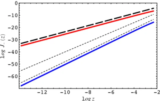
-12 -10 -8 -6 -4 -2 log z
-60 -50 -40 -30 -20 -10 0
l
og
J!
!
z
"
Figure 2: The boundary behaviour ofJ−(0) in for a generic solution (blue) to Eqs. (3.8) and a normalizable
Dirac-hair solution (red) for m = −1/4 in the background of an AdS-RN black hole with µ/T = 128.8.
The dotted lines show the scaling z11/2 and z4 of the leading and subleading terms in an expansion of
J−0(z) nearz= 0; the dashed line shows the scaling z5/2 of the subsubleading expansion whose coefficient
is|B−(ωF, kF)|2. That the Dirac hair solution (red) scales as the subsubleading solution indicates that the
current J−0 faithfully captures the density of the underlying normalizable Dirac field.
to a ground state with zero entropy, as hypothesized in [25]. This matches the expectation that the finite fermi-density solution in the bulk describes the Fermi-liquid. The underlying assumption in the above reasoning is that the total charge is conserved.
3.2.2 Finite fermion density in AdSS
For completeness, we will describe the finite fermion-density solutions in the AdS Schwarzschild geometry as well. In these solutions the charge density is set by the density of fermions alone. They are therefore not reliable at very low temperatures T Tc when gravitational backreaction
becomes important. The purpose of this section is to show the existence of finite density solutions does not depend on the presence of a charged black-hole set by the horizon value Φ(2)hor = µ0, but
that the transition to a finite fermion density can be driven by the charged fermions themselves. Fig. 4B shows the nearly instantaneous development of a non-vanishing expectation value for the occupation number discontinuity ∆nF andI in the AdS Schwarzschild background. The rise is not
as sharp as in the RN background. It is, however, steeper than exponential, and we may conclude that the system undergoes a discontinuous first order transition to a AdS Dirac hair solution. The constant limit reached by the fermion density as T → 0 has no meaning as we cannot trust the solution far away from Tc.
The backreaction due to the electric field divergence at the horizon can be neglected, for the same reason as before (Fig. 4C).
3.3 Confirmation from fermion spectral functions
(A)
−8.0 −7.0 −6.0 −5.0
−14
−13
−12
−11
−10
−9
−8
−7
log T/µ
log
!"
n F
/
µ
2
" #
!J0 −#$ T
−1.22
Charge density on the Fermi surface
Saturation at Fermi temperature
(B)
1 1.05 1.1 1.15 1.2 1.25 1.3 1.35 1.4
1 1.05 1.1 1.15 1.2 1.25 1.3 1.35 1.4 1.45 1.5
!
"
1 1.2 1.4
0 2 4
!
#
numerical exponents best linear fit " $ 0.84 !
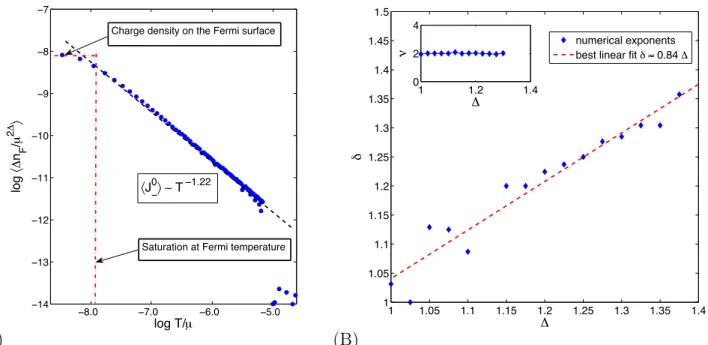
Figure 3: (A) Approximate power-law scaling of the Fermi liquid characteristic occupation number
discontinuity ∆nF/µ2∆∼T−δ as a function ofT /µ for ∆ = 5/4. This figure clearly shows the saturation
of the density at very low T /µ. The saturation effect is naturally interpreted as the influence of the
characteristic Fermi energy. (B) The scaling exponent δ for different values of the conformal dimension
∆. There is a clear correlation, but the precise relation cannot be determined numerically. The scaling
exponent of the currentI/µ2∆+1∼T−1/ν obeys ν = 2 with great accuracy, on the other hand (Inset).
the finite fermion density system is a more favorable state. This indeed follows from a detailed comparison between the spectral functions A(ω;k) in the probe limit and the fermion-liquid phase (Fig. 5). We see that:
1. All quasiparticle poles present in the probe limit are also present in the Dirac hair phase, at a slightly shifted value of kF. This shift is a consequence of the change in the bulk electrostatic
potential Φ due to the presence of the charged matter. For a Fermi-liquid-like quasipar-ticle corresponding to the second pole in the operator with ∆ = 5/4 and g = 2 we find
kFprobe−k∆nF
F = 0.07µ. The non-Fermi-liquid pole, i.e. the first pole for the same conformal
operator, has kFprobe−k∆nF
F = 0.03µ.
2. The dispersion exponentsνdefined through (ω−EF)2 ∼(k−kF)2/ν, also maintain roughly the
same values as both solutions. This is visually evident in the near similar slopes of the ridges in Fig. 5. In the AdS Reissner-Nordstr¨om background, the dispersion coefficients are known
analytically as a function of the Fermi momentum: νkF =
q 2kF2
µ2 −
1 3 +
1
6(∆−3/2) 2
[13]. The Fermi-liquid-like quasiparticle corresponding to the second pole in the operator with ∆ = 5/4 and g = 2 hasνkprobe
F = 1.02 vs. ν
∆nF = 1.01. The non-Fermi-liquid pole corresponding to the
first pole for the same conformal operator, has νkprobe
F ≈0.10, and ν
∆nF = 0.12.
(A)
0.2 0.4 0.6 0.8 1
0.99925 0.9995 0.99975 1 1.00025 1.0005 1.00075 z E!z"#E!1#2"
0.92 0.94 0.96 0.98 1
1.0002 1.0004 1.0006 1.0008 1.001 1.0012 1.0014 z E!z"#E!1#2"
(B)
! !"!# !"$ !"$# !"% !"%#
! $ % & '()$! !$% *+, ! - . +, % ! ) )
! !"!# !"$ !"$# !"% !"%#
! !"# $ $"# %()$! !/ *+, 0+, % ! 1$ ) ) 2345643789):3;;)<=8>37<> ?(=<-8-7@34)A@7 2345643789)56>>8-7)98-;@7B ?(=<-8-7@34)A@7 (C)
0.2 0.4 0.6 0.8 1
0.5 1 1.5 2 2.5 3 3.5 4 z E!z"#E!1#2"
0.92 0.94 0.96 0.98 1 2 2.5 3 3.5 4 4.5 5 z E!z"#E!1#2"
Figure 4: (A) The radial electric field −Ez = ∂Φ/∂z, normalized to the midpoint value Ez(z)/Ez(1/2)
for whole interior of the finite fermion density AdS-RN solution (upper) and near the horizon (lower). One clearly sees the soft, log-singularity at the horizon. The colors correspond to increasing temperatures
from T = 0.04µ (lighter) to T = 0.18µ (darker), all with ∆ = 1.1. (B) The occupation number jump
∆nF and free energy contributionI as a function of temperature in AdS-Schwarzschild. We see the jump
∆nF saturate at low temperatures and fall off at high T. An exponential fit to the data (red curve)
shows that in the critical region the fall-off is stronger than exponential, indicating that the transition is first order. The conformal dimension of the fermionic operator is ∆ = 1.1. (C) The radial electric
field−Ez =∂Φ/∂z, normalized to the midpoint value (Ez(z)/Ez(1/2)) for the finite fermion density
AdS-Schwarzschild background. The divergence of the electric fieldEz is again only noticeable near the horizon
and can be neglected in most of the bulk region.
by an order of magnitude. This suggests that the finite density state corresponds to the Fermi-liquid like state, rather than a non-Fermi liquid.
4. As we mentioned in the introduction, part of the reason to suspect the existence of an AdS-RN Dirac-hair solution is that a detailed study of spectral functions in AdS-AdS-RN reveals that the quasiparticle peak is anomalously sensitive to changes in T. This anomalous temperature dependence disappears in the finite density solution. Specifically in pure AdS-RN the position
ωmax where the peak height is maximum, denoted EF in [12], does not agree with the value ωpole, where the pole touches the real axis in the complex ω-plane, for any finite value of T,
and is exponentially sensitive to changes inT (Fig 6). In the AdS-RN Dirac hair solution the location ωmax and the location ωpole do become the same. Fig. 6B shows that the maximum
of the quasiparticle peak always sits at ω ' 0 in finite density Dirac hair solution, while it only reaches this as T →0 in the probe AdS-RN case.
4
Discussion and Conclusion
k/µ
!
/
µ
0 0.02 0.04 0.06 0.08 0.10 0.12 0.14 0.16 0.18 0.14
0.12
0.10
0.08
0.06
0.04
0.02
0 −6000
−4000
−2000
0 2000 4000 6000
k/µ
!
/
µ
0.05 0.06 0.07 0.08 0.09
−0.025
−0.020
−0.015
−0.010
−0.050
0
0.005
−0.025 −30000
−20000
−10000 0 10000 20000 30000
+ 42000
− 5200
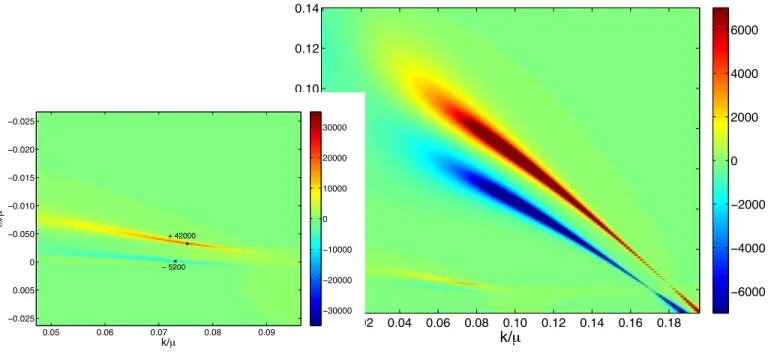
Figure 5: The single-fermion spectral function in the probe limit of pure AdS Reissner-Nordstr¨om
(red/yellow)minusthe spectrum in the finite density system (blue). The conformal dimension is ∆ = 5/4,
the probe charge g = 2, and µ/T = 135. We can see two quasiparticle poles near ω = 0, a non-FL pole
with kFprobe'0.11µand k∆nF
F '0.08µrespectively and a FL-pole with k
probe
F '0.18µand k
∆nF
F '0.17µ.
The dispersion of both poles is visibly similar between the probe and the finite density backgroudnd. At the same time, the non-FL pole has about 8 times less weight in the finite density background, whereas the FL-pole has gained about 6.5 times more weight.
it assumes the ground state it cannot explain its genericity. If the Fermi liquid ground state is so robust, this must also be a feature of the recent holographic approaches to strongly interacting fermionic systems. Our results here indicate that this is so: We have used Migdal’s relation to construct AdS/CFT rules for the holographic dual of a Fermi liquid: the characteristic occupation number discontinuity ∆nF is encoded in the normalizable subsubleading component of the spatially averaged fermion density J0
−(z) ≡
R
d3kΨ(¯ ω = 0,−k, z)iγ0Ψ(ω = 0, k, z) near the AdS boundary.
This density has its own set of evolution equations, based on the underlying Dirac field, and insisting on normalizability automatically selects the on-shell wavefunctions of the underlying Dirac-field.
The simplest AdS solution that has a non-vanishing expectation value for the occupation number discontinuity ∆nF is that of a single fermion wavefunction. Using the density approach — which
(A)
−0.020 −0.01 0
1 2 3
4x 10
6
!/µ
A(
!
,k)
T = 0.022µ
−0.020 −0.01 0
1 2 3
4x 10
7
!/µ
A(
!
,k)
−0.020 −0.01 0
1 2 3
4x 10
7
!/µ
A(
!
,k)
−0.020 −0.01 0
1 2 3
4x 10
6
!/µ
A(
!
,k)
T = 0.004µ
−0.020 −0.01 0
1 2 3
4x 10
6
!/µ
A(
!
,k)
T = 0.007µ
−0.020 −0.01 0
1 2 3
4x 10
7
!/µ
A(
!
,k)
(B)
0.190 0.195 0.200 0.205 0.210
−0.020 −0.015 −0.010 −0.005 0 k/µ ! / µ With backreaction Without backreaction
Figure 6: (A) Single fermion spectral functions near ω = 0 in pure AdS Reissner-Nordstr¨om (blue) and in the finite fermion density background (red). In the former the position of the maximum approaches
ω = 0 asT is lowered whereas in the latter the position of the maximum stays close toT = 0 for all values
of T. (B) Position of the maximum of the quasiparticle peak ink-ω plane, for different temperatures and
∆ = 5/4. The probe limit around a AdS-RN black hole (blue) carries a strong temperature dependence of
theωmaxvalue, withωmax,T6=06= 0. In the finite fermion density background, the position of the maximum
(red) is nearly independent of temperature and stays at ω= 0.
dependence present in the pure charged black-hole single spectral functions. This also indicates that the finite density state is the true ground state.
The discovery of this state reveals a new essential component in the study of strongly coupled fermionic systems through gravitational duals, where one should take into account the expectation values of fermion bilinears. Technically the construction of the full gravitationally backreacted solution is a first point that is needed to complete our finding. This is under current investigation. The realization, however, that expectation values of fermion bilinears can be captured in holographic duals and naturally encode phase separations in strongly coupled fermion systems should find a large set of applications in the near future.
Schalm) from the Netherlands Organisation for Scientific Research (NWO), a Spinoza Award (J. Za-anen) from the Netherlands Organisation for Scientific Research (NWO) and the Dutch Foundation for Fundamental Research on Matter (FOM).
References
[1] C. M. Varma, Z. Nussinov, W. van Saarloos, Singular Fermi Liquids Phys. Rep. 361, 267 (2002) [arXiv:cond-mat/0103393].
[2] J.H. She, J. Zaanen, BCS Superconductivity in Quantum Critical Metals, Phys. Rev. B80, 184518 (2009) [arXiv:0905.1225 [cond-mat]].
[3] H. v. L¨ohneysen, A. Rosch, M. Vojta, P. W¨olfle Fermi-liquid instabilities at magnetic quantum phase transitions, Rev. Mod. Phys.79, 1015 (2007) [arXiv:cond-mat/0606317 [cond-mat]]. [4] M. Gurvitch, A. T. Fiory, Resistivity of La1.825Sr0.175CuO4 and Y Ba2Cu3O7 to 1100 K:
Absence of saturation and its implications, Phys. Rev. Lett. 59, 1337 (1987).
[5] P. Phillips, C. Chamon, Breakdown of One-Paramater Scaling in Quantum Critical Scenarios for the High-Temperature Copper-oxide Superconductors, Phys. Rev. Lett. 95, 107002 (2005). [arXiv:cond-mat/0412179]
[6] J. Zaanen, Quantum critical electron systems: the unchartered sign worlds, Science319, 1205 (2008).
[7] J. M. Luttinger,Fermi Surface and Some Simple Equilibrium Properties of a System of Inter-acting Fermions, Phys. Rev. 119, 1153 (1960).
[8] J. C. Campuzano, M. R. Norman, M. Randeria, “Photoemission in the High-Tc
Supercon-ductors”, in Handbook of Physics: Physics of Conventional and Unconventional Superconduc-tors, edited by K. H. Benneman and J. B. Ketterson, (Springer Verlag, 2004); [arXiv:cond-mat/0209476]
[9] A. Damascelli, Z. Hussain, Z. X. Shen, Angle-resolved photoemission studies of the cuprate superconductors, Rev. Mod. Phys. 75, 473 (2003); [arXiv:cond-mat/0208504]
[10] X. J. Zhou, T. Cuk, T. Devereaux, N. Nagaosa, Z.-X. Shen, “Angle-Resolved Photoemission Spectroscopy on Electronic Structure and Electron-Phonon Coupling in Cuprate Superconduc-tors” in Handbook of High-Temperature Superconductivity: Theory and Experiment, edited by J. R. Schrieffer, (Springer Verlag, 2007); [arXiv:cond-mat/0604284]
[11] H. Liu, J. McGreevy, D. Vegh, Non-Fermi liquids from holography, arXiv:0903.2477 [hep-th]. [12] M. ˇCubrovi´c, J. Zaanen, K. Schalm,String Theory, Quantum Phase Transitions and the
Emer-gent Fermi-Liquid, Science 325, 439 (2009) [arXiv:0904.1993 [hep-th]].
[13] T. Faulkner, H. Liu, J. McGreevy, D. Vegh, Emergent quantum criticality, Fermi surfaces, and AdS2, arXiv:0907.2694 [hep-th].