An algorithm for enhancing coverage and network
lifetime in cluster-based Wireless Sensor Networks
Walid Osamy
1and Ahmed M. Khedr
21
University of Benha, Faculty of Computers and Informatics, Dept. of Computer Science
2
University of Sharjah, College of Sciences, Dept. of Computer Science
2
Zagazig university, Faculty of Science, Mathematics Department
Abstract: Majority of wireless sensor networks (WSNs) clustering protocols in literature have focused on extending network lifetime and little attention has been paid to the coverage preservation as one of the QoS requirements along with network lifetime. In this paper, an algorithm is proposed to be integrated with clustering protocols to improve network lifetime as well as preserve network coverage in heterogeneous wireless sensor networks (HWSNs) where sensor nodes can have different sensing radii and energy attributes. The proposed algorithm works in proactive way to preserve network coverage and extend network lifetime by efficiently leveraging mobility to optimize the average coverage rate using only the nodes that are already deployed in the network. Simulations are conducted to validate the proposed algorithm by showing improvement in network lifetime and enhanced full coverage time with less energy consumption.
Keywords: Heterogeneous wireless sensor Networks, Clustering Protocols, Network lifetime, Energy consumption, Coverage preservation, full coverage time.
1.
Introduction
How to maximize network lifetime and maintain good coverage for network area for as long as possible using as minimum energy as possible?. The answer to this question is the main issue in WSNs. In other words, one of crucial issues in WSNs is saving energy that is to maximize network lifetime. As a result, the design of energy efficient methods for WSNs is one of the main research challenges in WSNs that is addressed by a large number of literature during the last few years. Therefore, it is required that the WSNs that are deployed with high node densities save their energies by turning off sensor nodes that have overlapping sensing areas for energy efficiency and to extend network lifetime. Moreover, coverage in WSNs is to monitor network field in an efficient way which means using as minimum energy as possible to ensure good coverage for as long as possible. Clustering is one of the most used methods in WSNs for saving energy and extending network lifetime.
In clustering methods, nodes are often partitioned based on some criteria into various disjoint groups called clusters. Clustering in WSNs reduces communication overheads and allocates resources effectively as a result overall energy consumption and interference among nodes is reduced, [3, 5– 7].
Clustering algorithms apply data aggregation techniques, which reduce the collected data at cluster heads in form of significant information, [2, 3, 5]. Most clustering protocols in literature have focused on the ways of cluster heads selection and cluster formation or how to route the aggregated data from nodes to the base station to extend network lifetime. Very little clustering work pays attention to coverage preservation besides extending network lifetime. For this reason, in this paper, we propose an enhancement algorithm
that can be integrated with clustering protocols for HWSNs to enhance coverage and network lifetime. The new protocol starts (Initialization phase) by selecting suitable nodes to be activated for sensing and aggregation process from the nodes that are already deployed in the network. During sensing process, node energy level is monitored in order to recover the nodes that reach a certain energy threshold value (Coverage preservation phase).
In the recovery process, the neighbor nodes collaborate among themselves to find the most appropriate candidate based on sensing range, residual energy, and required moving distance (Coverage preservation phase).
The selected node then will move to replace the failed node. The new protocol minimizes any overlapping of the selected node with its new neighbors in the target location, improves the coverage of its predecessor, and efficiently leverages mobility to optimize the average coverage rate [1].
The rest of the paper is organized as follows: Section 2 describes related research on our proposed work. In section 3, we give a number of related definitions and notations that will be used in developing our algorithms. In Section 4, we introduce our approach to carry out the proposed problem. The simulation of our approach is presented in Section 5. In Section 6, we conclude our work.
2.
Related Research
In this section, we review the recent works dealing with the coverage preservation and network lifetime maximization in cluster based WSNs. In [3], the authors proposed Deterministic Energy-efficient Clustering protocol (DEC) which uses residual energy of nodes to select cluster heads in a deterministic way. The performance is measured in terms of lifetime and coverage preservation under energy heterogeneity. DEC outperforms the probabilistic-based protocol LEACH. In [4], the authors proposed two distance based clustering routing protocols, DBLEACH and DBEA-LEACH.
In DBLEACH, the cluster head selection is based on the distance between the candidate node and the base station. While in DBEA-LEACH the cluster head selection is not only based on the distance between the candidate node and the base station, but also the ratio of residual energy of the node and the average residual energy level of nodes in the network.
EBCM considers current node energy and degree in cluster formation process that is to overcome the energy limitation and imbalance of energy consumption among sensor nodes. In [1] Region-based Energy-aware Clustering (REC) scheme is proposed for packet forwarding in WSNs. REC stresses the residual energy and the sensing coverage area as metrics for cluster head selection. The work in [4] ignored area coverage improvement with minimal energy consumption and concentrated only on cluster head selection even if the algorithm is based on area coverage but this is to extend network lifetime which is indirectly related to coverage preservation.
In [24], the authors proposed a coverage optimization protocol to improve the lifetime in heterogeneous WSNs. The network area is divided into sub-regions then the scheduling of sensor node activity is planned for each sub-region. In [11], the authors presented an energy and coverage-aware distributed clustering protocol (ECDC). They proposed two important coverage cost metrics aimed at mitigating different applications of a coverage problem, particularly including an area coverage problem. Here, coverage cost is proportional to the number of neighbors. ECDC cannot efficiently extend the network lifetime. In [10], the authors proposed a distributed, energy and coverage-aware routing (DECAR) algorithm to improve coverage lifetime.
They proposed a cluster-size selection technique with the objective of minimizing the problem of hot spots during data transmission to the BS. Although, the performance is improved, this algorithm does not address sensor activation, but it focuses only on clustering optimization. In [13], the authors proposed the Edge Based Centroid (EBC) algorithm which aims to improve the area coverage with minimal energy consumption and faster convergence rate. In [17], a distributed coverage hole detection scheme is proposed in which the sensors can store location information of their one-hop neighbors to detect the presence of a coverage hole without the help of the sink.
In context of hole recovery, the approach in [18] locates the shortest moved distance of the mobile nodes. Then using an adaptive threshold distance, the algorithm filters out some mobile nodes that are already occupied or situated within the threshold distance from the optimal new positions. The work in [14] proposed an algorithm to improve coverage of a hole by moving nodes but with heavy constraints on energy and distance. Authors in [12] discussed how improve the network coverage by redeploying mobile nodes in hybrid WSNs. In [15], the authors proposed a coverage hole repair algorithm to resolve a full coverage while minimizing the overlapped area of the sensing disks and deployed nodes. In [16], the authors used a hybrid particle swarm algorithm to repair the coverage holes. In these approaches, the movement of mobile sensors and the consumption and balancing energy are studied. However, these approaches are based on the homogeneous WSNs, which is not the case of our proposed problem. In [8], the authors presented a pruning-based algorithm, where nodes are considered to be redundant if their sensing regions are covered by other neighbors, and their neighbors are connected through a connection path. This algorithm works with homogenous sensor nodes. The work in [1] is close to ours. However, our approach is based on local neighborhood information and is based on different assumptions.
3.
Description of Relevant Terms
In this section, we give some definitions and notations that will be used in developing our proposed algorithm. We consider that there are n sensor nodes that are randomly scattered over a monitored area, and they form the set , where Also, we assume that the application requires every part of the area to be covered by the sensors throughout the network lifetime, i.e., sensor nodes are deployed in high density to ensure full coverage. Moreover, the WSN has the following assumptions:
1. Every sensor node knows its own location via GPS or localization algorithms
[2, 19]
.2. A Boolean disk coverage model is considered as this model is widely used in literature.
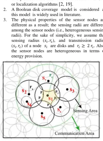
3. The physical properties of the sensor nodes are different as a result; the sensing radii are different among the sensor nodes (i.e., heterogeneous sensing radii). For the sake of simplicity, we assume that sensing radius ( ), and transmission radius ( ) of a node are disks and . Also, the sensor nodes are heterogeneous in terms of energy provision.
Figure 1. Example of Heterogeneous WSN
Definition 1 (Communication Area): The communication area of a sensor node ( ) is the area in which the sensor can communicate directly with other sensor nodes. Definition 2 (Communication Neighbors): The communication neighbors of a sensor node ( ) are represented by the set of all sensor nodes which are located inside .
Definition 3 (Sensing Area): The sensing area (sensing disc) of a sensor node ( ) is the area in which the sensor can sense a physical phenomenon for example moving object.
Definition 4 (Sensing Neighbors): The Sensing neighbors of a sensor node ( ) are represented by the set of all sensor nodes s that satisfy the condition . As shown in Figure 1, the sensing neighbors of are represented by the set .
For example, in Figure 1, and the number of nodes in the list is 1 ( ).
Definition 6 (Coverage Hole): If any part of the monitoring region is not covered by the sensing disc of any sensor, then there exists a coverage hole.
Definition 7 (Hole Boundary Points (HBP)): HBPs are the intersection points of nodes' sensing discs around a coverage hole, which develop an irregular polygon by connecting adjacent points. As shown in Figure 1, the shadowed area is expected to be a coverage hole with
if node dies.
Definition 8 (Hole Boundary Nodes (HBN)): HBN are the nodes that form the boundary of the hole. As shown in Figure 1, the shadowed area is expected to be a coverage hole with if node dies.
4.
Algorithm Description
Our main objectives it to preserve maximal coverage and extend network lifetime. Therefore, we propose an algorithm that is divided into two phases: initialization, and coverage preservation. In initialization phase, each node collects and determines the required information about its vicinity (e.g., sensing neighbors) that is used as preparation for the next phase. Moreover, redundant nodes are discovered and scheduled for coverage preservation and energy saving. In coverage preservation phase, node whose energy level goes under a certain energy threshold value will be replaced by selecting the most convenient node to avoid the expected coverage hole. This selection will be decided by the node with low energy level.
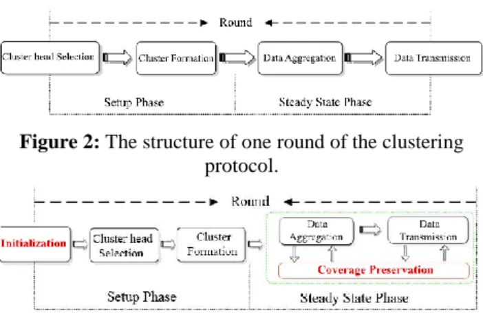
Figure 2: The structure of one round of the clustering protocol.
Figure 3: Modified structure of one round of the clustering protocol.
Cluster based protocols for WSNs are divided into rounds and each round has two main phases, setup phase and data collection phase or steady state phase as show in Figure 2. In cluster formation phase, cluster heads are selected based on their local information (e.g., residual energy) or based on predefined probability (cluster head selection step). Then nodes cooperate with the elected cluster heads to form a cluster (cluster formation step). While, in data collection phase cluster member nodes send their data to cluster head nodes. Cluster head nodes then send the aggregated data to the base station.
Our proposed algorithm will be integrated with clustering protocols and the round structure will be modified. As it is seen in Figure 3, the new round structure begins with our initialization phase and the coverage preservation phase will
be executed concurrently with data aggregation and data transmission steps in steady state phase. Here, we start with the description of the initialization phase, and then we present the full description of the coverage preservation phase.
4.1 Initialization Phase
Each node enters this phase after deployment or after changing its location. In this phase, each node will execute the following procedure that includes three steps:
1. Finding sensing neighbors. 2. Finding redundant neighbors. 3. Determining intersection points. Step 1: Finding Sensing Neighbors
In this step finds its sensing neighbor nodes as follows: For each node , will be added to sensing neighbor list, , if the distance between and is less than or equal to .
Step 2: Finding Redundant Neighbors
Considering only its sensing area, the coverage redundancy ratio for each node can be calculated using
[9, 20]
as follows:
4.1
where, is the sensing area of that has been covered by neighbor node , and is the sensing area of .
1. If , no coverage redundancy for . 2. If > 0 and <1 coverage redundancy occurred
with .
3. If , sensor has a complete coverage redundancy.
Let is a redundancy threshold that depends on the
application.
According to equation 4.1, if node has , and
has a neighbor with as result if both of
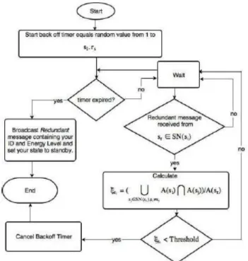
them decide to become redundant node and go to sleep, it may cause two problems: (1) a coverage hole will occur at the shared region, (2) both of them will receive move request during recovery process and this will cause a coverage hole. Each node executes Algorithm 1 to decide whether to become a redundant node and go to sleep mode or not. The idea of the algorithm is that each node starts backoff timer (its value is a random number from 1 to ) and if it receives Redundant message before its timer expires, it checks if it still has or not after excluding
the node that sends the declaration message from calculation of its . If , it decides to cancel
its timer and does not declare itself as redundant node. Otherwise, it declares itself as redundant node and goes to standby mode after timer expiration. Each node that receives Redundant message from ; adds to its redundant list . Figure 4 shows the flow diagram for redundant discovery algorithm.
Step 3: Determining Intersection Points
The intersection points and between nodes with sensing radius and with sensing radius can be computed as follows:
Figure 4: Flow Diagram of Redundant Discovery Algorithm.
(4.2)
(4.3)
where, is the distance between and such that
or ,
The points ( , ) will be added to the list of intersection points ( ).
Find the intersection points between each pair of sensing neighbors , ( ).
Add these points to the list of intersection points
.
For each point , update with the number of nodes that cover by counting the number of corresponding sensing neighbors
that cover .
The intersection point that is covered by more than one nodes is not a hole boundary point; otherwise it is a hole boundary point.
The intersection point that is covered by only is expected to be hole boundary point if dies.
At the end of this phase, each node has to maintain the list of its sensing neighbors' information and corresponding intersection points.
4.2 Coverage Preservation Phase
In this phase, the energy level of sensor node is monitored and if the remaining energy of node ( ) is less than a given energy threshold , i.e. is expected to die and
cause a coverage hole. In this case, considers itself as hole coordinator node and prepares to execute the recovery algorithm by finding the list of hole boundary points
for that expected hole by picking the points that are covered only by itself from and adds them to list.
The recovery algorithm works reactively for the hole resulting due to node failure. The boundary hole nodes and the hole can be detected using the related methods presented in previous studies e.g., [23] . The set of nodes that are located on the hole boundary, compute the intersection points with hole boundary neighbors to update their
list. The hole boundary nodes exchange their s along with their IDs and the node with lowest ID considers itself the hole coordinator node and will execute recovery algorithm.
First, we describe selection procedure for selecting the candidate redundant node to move and recover the hole, then we provide the details of the recovery algorithm.
4.2.1 Candidate Selection Procedure
In order to select candidate node to move towards coverage hole or to preserve coverage, the coordinator node finds the smallest circle that encloses the points in the list to recover the hole. Then, searches for the candidate node (redundant node) that has sensing radius greater than or equal to the radius of the smallest enclosing circle. The candidate node then will be moved to the center of smallest enclosing circle.
However, the selection based on sensing radius only could lead to selection of a node that has not enough energy to complete this task. Therefore, the selection of candidate node must be based on more factors. In this paper, we consider three main factors to select a candidate node: required sensing radius, moving distance, and remaining energy. If we assume the energy consumed to move a node distance is and the remaining energy of is . Node calculates the following energy-distance factor ( ) for each of its candidate nodes ( ).
(4.4)
The candidate node that has and is the most convenient node to move and
cover, where is energy-distance
factor threshold, is the energy threshold and
is the required radius.
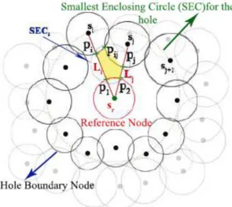
Figure 5: Coverage hole example with reference node.
Figure 6: Dividing example for the area between reference node and hole boundary node.
Figure 7: Covered area between reference node and hole boundary nodes.
4.2.2 Hole Recovery Algorithm
Here, hole recovery algorithm is described in order to preserve and extend network coverage. As stated before, we have two cases. In case 1, the node attempt to recover the coverage hole before it becomes a real problem by monitoring its energy level till it reaches certain energy threshold value. In case 2, the coverage hole is detected and the hole boundary node that has lowest ID becomes hole coordinator node and maintains list for the hole. In both cases the hole coordinator node executes the recovery algorithm.
The main idea of the algorithm is that given a set of hole boundary points, , the points in are sorted in counterclockwise. Hole coordinator node executes the following steps:
1. Find the smallest enclosing circle ( ) for the hole points in the list by executing the algorithm in [21, 22].
2. Search in the RN list for a redundant node by calling candidate selection procedure , if it exists; the redundant node will be requested to move to
center. Terminate the algorithm. (The nearest one from center will be selected if there are more than one redundant nodes that can fit to the radius of ).
3. If there is no redundant node that can fit to the hole and the redundant list contains only one node ( ), decides to send request to neighbor nodes asking them for redundant list. 4. updates its redundant list by the received list
nodes then call candidate selection procedure to search for a redundant node with radius greater than or equal to the radius of in the updated redundant list.
5. If it exists; the redundant node will be requested to move to center and then updates its redundant list.
6. If no update is received, node sends the hole information to base station that includes hole center (SEC center) and size (SEC radius) and terminates the algorithm.
7. If all redundant nodes in have radius less than the radius of , selects the node that has largest sensing radius and
as reference node for the hole.
8. requests the reference node to move to the hole center (SEC center) then, will execute the following:
a. Finds the line from the center of to the center of reference node and the line
from the center of hole boundary neighbor node to the center of reference node .
b. Finds the intersection points of and with the circumference of the reference node .
c. Finds the intersection points of and with the circumference of the hole boundary node .
and the point is the intersection between
and . These points form polygon that encloses a hole. The coordinates of cross point can be calculated as follows:
(4.5)
(4.6)
where is the distance between the center of node and the center of node , and is the sensing radius of . By the same way the other cross points can calculated.
9. finds the smallest enclosing circle ( ) for the cross points and the intersection point between and ( as shown in Figure 5, is the smallest enclosing circle for the intersection point and
the points ).
10. searches for the redundant node by calling candidate selection procedure that matches . 11. If exists; will be requested to move to the
position of center then updates its by removing from the list.
12. sends the hole information ( , reference node, covered area) to its node . repeats the same processes (starts from step 9) between itself and hole boundary nodes .
13. But, if the node cannot find In this case, will divide the area that needs to be covered by redundant nodes as follows:
a. finds the mid points , of and
, respectively. As shown in Figure 6, the polygon , , , , is divided into
two polygons , , , , and ,
, , by the mid points.
b. finds the smallest enclosing circle ( ) for the polygon points , , , , and the smallest enclosing circle
( ) for the polygon point , , ,
.
c. searches for the redundant nodes and that match and by calling
candidate selection procedure; d. will be requested to move to the
position of center and will be
requested to move to the position of
center.
14. updates its by removing from the lists, then sends the hole information ( ,
reference node, covered area) to its node . 15. Node repeats the same processes (starts from
step (8.a) between itself and hole boundary nodes
.
5.
Simulation Results
The proposed algorithm was simulated using MATLAB with the same radio model and the energy parameter used as in the literature [2–5]. In our simulation, 100 sensor nodes are uniformly distributed in a region of size .
The sensing range varies between 15m and 30m and communication range is taken to be 60m. The cluster head probability is set to 0.10 with base station located at center of simulation area. The initial energy is varying from 20J to 50J, energy consumption due to mobility is taken to be 1 J/m. We set energy threshold equals to 10% of initial energy of each node and the coverage threshold value
.
The simulation is run for different topologies and average value of all runs is presented in the simulation result. The simulated parameters are summarized in Table 1.
The proposed algorithm is analyzed by integrating it with these clustering protocols: Distance-Based Energy-Aware Low Energy Adaptive Clustering Hierarchy (DBEA-LEACH) [4], Distance-Based Low Energy Adaptive Clustering Hierarchy (DB-LEACH) [4], LEACH-E [2], Energy-Based Clustering Model (EBCM) [5] and Deterministic Energy-efficient Clustering protocol (DEC) [3]. We measure the performance by using the following metrics for clustering protocols without the proposed algorithm (DBEA-LEACH,
DB-LEACH, LEACH-E, EBCM, and DEC) and clustering protocols after the proposed algorithm is integrated into them (Modified-DBEA-LEACH, Modified-DB-LEACH, LEACH-E, EBCM, and Modified-DEC).
Full Coverage-Time [3]: the period from the start of the network operation until full coverage is lost.
Network Lifetime [2–4]: the period from the start of the network operation until the first node dies(FND).
Average Number of Active Nodes (ANAN) Ratio : The network lifetime and full coverage time is maximized when as few as possible number of active nodes are used in each round. As a result the minimum value of ANAN is preferred. ANAN is calculated as follows:
where, is the total number of nodes, is
the total number of active nodes until first node dies, and is the total number of active
nodes until full coverage is lost.
Averaged Consumed Energy per round: this metric is preferred to minimize the following:
o Averaged Consumed Energy per round until first node dies ( ). It is
calculated as:
where is the total consumed
o Averaged Consumed Energy per round until full coverage is lost ( ).
It is calculated as:
where is the total consumed
energy until full coverage is lost and
is the total number of rounds
until full is coverage lost.
Figures 8, 9 and 10 show the evolution for (DBEA-LEACH, DB-LEACH, LEACH-E, EBCM, and DEC) and (Modified-DBEA-LEACH, Modified-DB-LEACH, Modified-LEACH-E, Modified-EBCM, and Modified-DEC) over rounds in one set of the simulations. From Figure 10 we can see that the consumed energy per round for modified protocols is more balanced and less than original protocols.
Also we can see from Figure 9 that number of dead nodes per round decreased for modified protocols compared with the number of dead per round for original protocols. Moreover, from Figure 8 it is shown that the coverage percentage per round is improved for modified protocols compared with the original protocols.
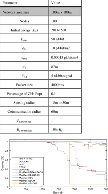
Table 1. Setting used in the simulation
Parameter Value
Network area size 100m x 100m
Nodes 100
Initial energy ( ) 20J to 50J
50 nJ/bit
10 pJ/bit/m2
0.00013 pJ/bit/m4
87m
5 nJ/bit/signal
Packet size 4000bits
Percentage of CHs Popt 0.1
Sensing radius 15m to 30m
Communication radius 60m
1
10%
Figure 8: Coverage performance of cluster protocols: DBEA-LEACH, DB-LEACH, DEC, EBCM, LEACH-E
before and after integrating.
Figure 9: Network lifetime performance of cluster protocols: DBEA-LEACH, DB-LEACH, DEC, EBCM, LEACH-E before and after integrating our proposed algorithm.
Figure 10: Consumed energy per round by protocols: DBEA-LEACH, DB-LEACH, DEC, EBCM, LEACH-E before and after integrating our proposed algorithm.
Figure 11: Average Consumed Energy by the protocols: DBEA-LEACH, DB-LEACH, DEC, EBCM, LEACH-E before and after integrating our proposed algorithm..
Figure 11 shows the average consumed energy per round until first node dies and until full coverage is lost. As shown from the figure that the average energy per round until first node dies is reduced up to a magnitude of 84.59%, 93.25%, 94.29%, 88.13%, and 96.26% for DEC, Modified-DBEA-LEACH, Modified-DB-LEACH, Modified-EBCM, and Modified-LEACH-E compared with DEC, DBEA-LEACH,
DB-LEACH, EBCM, and LEACH-E, respectively. Moreover, the average energy per round until full coverage is lost is reduced up to a magnitude of 78.05%, 81.07%, 88.63%, 81.18%, and 90.60% for DEC, Modified-DBEA-LEACH, Modified-DB-LEACH, Modified-EBCM, and Modified-LEACH-E compared with DEC, DBEA-LEACH, DB-DBEA-LEACH, EBCM, and LEACH-E, respectively. Moreover from Figure 11, it is clear that for original protocols DBEA-LEACH gives lowest and
protocols Modified-EBCM gives largest and
Modified-DBEALEACH gives lowest .
for all modified protocols is less than
for all original protocols. This is because the
number of active nodes per round for modified protocols is less than the number of active nodes per round for original protocols as a result we save energy.
Furthermore, we notice that is less than
for original protocols, while, is
greater than for modified protocols. This is
because shorter full coverage time in original protocol leads to increase in . However, longer full coverage
time in modified protocols lead to decrease in
with slight increase in due to the
movement of nodes to maintain the full coverage.
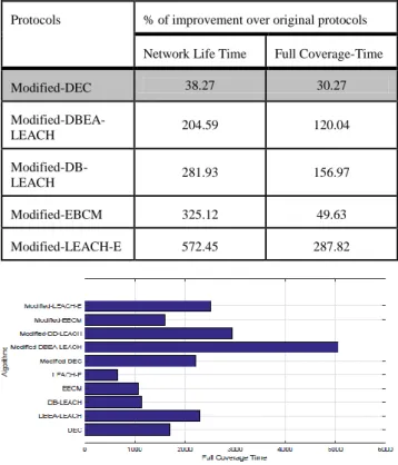
Table 2, shows the percentage of improvement of modified protocols over original protocols.
Table 2. Performance improvement over original protocols.
Protocols % of improvement over original protocols
Network Life Time Full Coverage-Time
Modified-DEC 38.27 30.27
Modified-DBEA-LEACH 204.59 120.04
Modified-DB-LEACH 281.93 156.97
Modified-EBCM 325.12 49.63
Modified-LEACH-E 572.45 287.82
Figure 12: Average Full Coverage-Time for protocols: DBEA-LEACH, DB-LEACH, DEC, EBCM, LEACH-E Before and after integrating our proposed algorithm...
Figure 13: Average Network Lifetime for protocols: DBEA-LEACH, DB-DBEA-LEACH, DEC, EBCM, LEACH-E before and after integrating our proposed algorithm.
As shown in Figure 12 and Figure 13, where the full coverage time and network lifetime are plotted for all
protocols. LEACH-E has a shorter coverage period and network lifetime compared with the other protocols, while Modified-DBEA-LEACH has a longer network lifetime and full coverage time compared with the other protocols. Modified-DEC performs better than DEC up till about 38.3% for network lifetime and 30.3% for full coverage time, Modified-LEACH performs better than DBEA-LEACH up till about 204% for network lifetime and 49% for full coverage time, and Modified-DB-LEACH performs better than DB-LEACH up till about 281.9% for network lifetime and 120% for full coverage time.
Similarly, Modified-EBCM performs better than EBCM up till about 325% for network lifetime and 49.5% for full coverage time and Modified-LEACH-E performs better than LEACH-E up till about 572.5% for network lifetime and 287.8% for full coverage time.
From Figure 13 and Figure 12, modified protocols have a clear cut advantage over original protocols, this is because each clustering protocol begin its setup phase after the execution of Redundant Discovery Algorithm which minimizes the number of active node that form clusters and data aggregation. Moreover, full coverage is extended as a result of coverage preservation phase in each round pro-actively recovering the expected dead node.
By comparing the results in Figure 13 with the results in Figure 12, it is noted that the full coverage time for all protocols is greater than the network lifetime.
Figure 14: Average active nodes ratio for the protocols: DBEA-LEACH, DB-LEACH, DEC, EBCM, LEACH-E before and after integrating our proposed algorithm.
In order to save energy, minimize communication overhead and extend network lifetime, it is desirable in each round to have as few working nodes as possible. Figure 14 shows the superiority of proposed algorithm in comparison with original protocols. Moreover, as it is shown in Figure 14 that
for all original protocols is greater than
as large number of active nodes start
clustering process and decrease in is because
the number of dead nodes may not affect full coverage as they are covered by neighbor nodes.
While for all modified protocols is lower than
because less number of active nodes start
clustering process. Furthermore, is slightly
increased since more active nodes are required for coverage preservation.
6.
Conclusions
algorithm takes the benefit from the nodes that are already deployed in the network and discover the redundant nodes. The redundant nodes are used for coverage preservation. The proposed algorithm can be integrated with clustering routing protocols to provide robust functionalities in WSN applications, which are highly desirable for surveillance applications that require persistent coverage and continuous surveillance in order to satisfy a specific quality of service (QoS) constraint. The proposed algorithm is integrated in DEC, DBEA-LEACH, DB-LEACH, EBCM, and LEACH-E and the performance results show that the modified protocols exceed the original protocols in terms of full coverage time, network lifetime, active number of nodes, and energy consumption.
References
[1] H. Hasbullah and B. Nazir, "Region-based Energy-aware cluster (REC) for efficient packet forwarding in WSN," International Symposium on Information Technology, Kuala Lumpur, 2010, pp. 1-6, 2010.
[2] D. Peng and Q. Zhang, "An energy efficient cluster-routing protocol for wireless sensor networks," International Conference On Computer Design and Applications, Qinhuangdao, 2010, pp. 530-533, 2010.
[3] F. A. Aderohunmu, Optimisation of Energy-efficient Transmission Protocol forWireless Sensor Networks (Thesis, Doctor of Philosophy). University of Otago. Retrieved from http://hdl.handle.net/10523/4455, 2013.
[4] T. G. Nguyen, C. So-In and N. G. Nguyen, "Two energy-efficient cluster head selection techniques based on distance for wireless sensor networks," 2014 International Computer Science and Engineering Conference (ICSEC), Khon Kaen, pp. 33-38, 2014. [5] Z. Fan, M. Cai, X. Li and J. Chen, "A New Dynamic Energy Based Clustering Model for Wireless Sensor Networks," IEEE International Conference on Computational Science and Engineering (CSE) and IEEE International Conference on Embedded and Ubiquitous Computing (EUC), Guangzhou, 2017, pp. 619-622, 2017.
[6] A. Salim, W. Osamy, and A. M. Khedr, "IBLEACH: Effective LEACH Protocol for Wireless Sensor Networks," Wireless Networks, Vol. 20, pp. 1515-1525, 2014.
[7] A. M. Khedr, and W. Osamy, "Target tracking Mechanism for Cluster Based Sensor Networks", Applied Mathematics and Information Science Journal, vol. 1, no. 3, pp. 287- 303, 2007. [8] A. K. Datta, M. Gradinariu, and R Patel, "Distributed self* minimum connected covering of a query region in sensor networks," In ISPAN ’05, pp. 448-453, 2005.
[9] F. Librino, M. Levorato and M. Zorzi, "An Algorithmic Solution for Computing Circle Intersection Areas and its Applications to Wireless Communications", arXiv:1204.3569 [cs.CG], 2012.
[10] T. Amgoth, PK Jana, "Energy and coverage-aware routing algorithm for wireless sensor networks," Wirel Pers Commun vol. 81, no. 2, pp.531-545, 2015.
[11] X. Gu, J. Yu, D. Yu, G. Wang, Y. Lv, ”ECDC: An energy and coverage-aware distributed clustering protocol for wireless sensor networks," Comput Electr Eng vol.40, no. 2, pp. 384-398, 2014. [12] Q. Zhang, M. P. Fok, "A Two-Phase Coverage-Enhancing Algorithm for Hybrid Wireless Sensor Networks," Sensors, vol. 17, pp. 117, 2017
[13] M. S. Aliyu, A. H. Abdullah, H. Chizari, T. Sabbah, A. Altameem, ”Coverage enhancement algorithms for distributed mobile sensors deployment in wireless sensor networks," International Journal of Distributed Sensor Networks, 2016. [14] B. Manoj, A. Sekhar, and C. Siva Ram Murthy, ”On the use of limited autonomous mobility for dynamic coverage maintenance in sensor networks," Computer Networks, vol. 51, no. 8, pp.2126-2143, 2007.
[15] L. Aliouane, M. Benchaiba, ”HACH: Healing Algorithm of Coverage Hole in a Wireless Sensor Network," Proceedings of the 2014 Eighth International Conference on Next Generation Mobile Apps, Services and Technologies (NGMAST); pp. 215-220, Oxford, UK., 10-12 September 2014.
[16] X. Fan, Z. Zhang, X. Lin, H.Wang, ”Coverage hole elimination based on sensor intelligent redeployment in WSN," Proceedings of the 2014 IEEE 4th Annual International Conference on Cyber Technology in Automation, Control, and Intelligent Systems (CYBER), pp. 336-339, Hong Kong, China, 4-7 June 2014. [17] K. Sahoo, M-J. Chiang, S-L. Wu,”An Efficient Distributed Coverage Hole Detection Protocol for Wireless Sensor Networks," Sensors, vol. 16, no. 3, pp. 386, 2016.
[18] A. M. Htun, M. S. Maw, I. Sasase, ”Reduced complexity on mobile sensor deployment and coverage hole healing by using adaptive threshold distance in hybrid Wireless Sensor Networks," Personal, Indoor, and Mobile Radio Communication (PIMRC). In Proceedings of the 2014 IEEE 25th Annual International Symposium on Capital Hilton, Washington, DC, USA; pp. 1547-1552, 2014.
[19] C. Cheng, C. Tse, F. Lau, ”A delay-aware data collection network structure for wireless sensor networks,"
IEEE Sensors Journal vol. 11, no. 3, pp.699-710, 2011.
[20] D. Izadi, J. Abawajy, and S. Ghanavati, ”An Alternative Node Deployment Scheme for WSNs," IEEE SENSORS JOURNAL, vol. 15, no. 2, pp. 667-675, 2015.
[21] E. Welzl, "Smallest enclosing disks (balls and ellipsoids)," New results and new trends in computer science, pp. 359-370, 1991.
[22] L. Xiang, and M. Fikret Ercan. "An Algorithm for Smallest Enclosing Circle Problem of Planar Point Sets." International Conference on Computational Science and Its Applications. Springer International Publishing, 2016.
[23] C. Zhang, Y. Zhang, Y. Fang. Localized Algorithms for Coverage Boundary Detection in Wireless Sensor Networks. Wirel Netw, vol. 15, no. 1, pp. 3-20, 2009.