An Analysis Nomoto Gain and Norbin Parameter on Ship Turning Maneuver

IPTEK, The Journal for Technology and Science, Vol. 21, No. 2, May 2010

Abstract

—

Keywords

—

I.INTRODUCTION

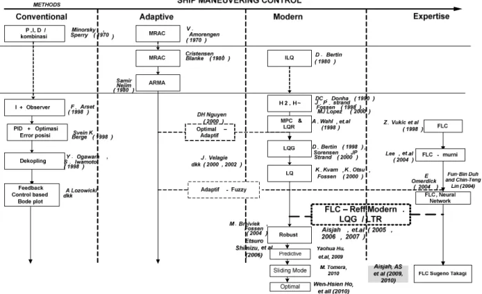
ome researches on ship maneuvering control have developed from 1946 until today [3]. Autopilot system has been applied on several ships including the ship Zuidweg (1970), Gaeta Class Minehunter (1970), Ferry - Massarenas (1996), Northern Clipper (1996) and Shioji Maru (2000). Various strategies in the design of the autopilot, i.e. with a conventional control strategy include adaptive, modern and expertise-based [11]. The development of this control system block diagram is depicted in Fig. 1.

A design of fuzzy logic based control system (FLC) strategy is proposed by using determinations of control-rules based on the performance of reference [10]. Reference control system LQG / LTR having been shown to have robust properties is tested against 19 types of ships with a length of 40-350 meters. Response control system shows the pattern of first order and second order. By analyzing the results of this response, parameters namely time constant system, gain, settling time for the system with the pattern of first order and the value of natural frequencies, damping ratio for systems with second order patterns-can be determined. Based on these parameters, constant gain Norbin Nomoto and parameters can be determined. Norbin parameter refers to a parameter that determines the ability to maneuver.

1_{Aulia Siti Aisjah is with Department of Physics Engineering, FTI,}

Institut Teknologi Sepuluh Nopember, Surabaya, 60111, Indo-nesia. E-mail: [email protected]

II.SHIP MANEUVERING CONTROL

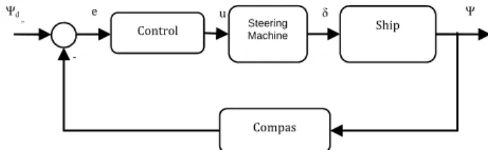
Ship maneuvering Control has been progressing very rapidly. Fig. 1 below indicates some strategies in conventional maneuver control, adaptive, modern and expertise based. Block diagram of a conventional control system is shown in Fig. 1 below:

Fig. 1. Block diagram of convensional control system

Conventional control system designed by some researchers has found many weaknesses; among others are disability to accommodate the interference with high frequency although a wave filter design as shown by Lozowicki and Tiano (2000) has been added. Interference from the environment causes changes in parameters of the controlled system, and this is the reason why this strategy is called adaptive control. In adaptive control systems, mathematical models such as one derived from conventional method in which additional variables are given are derived from the environment; furthermore, a mathematical model of this modification is expressed in various models called MRAC (Model Refference Adaptive Control) by Van Amorengen (1970) and Blanke (1980) and ARMA (Auto Regresive Moving Average) submitted by Nejim, (1998). The method proposed by Van Amorengen (1970) shows the results that are not linear on the rudder;in addition, it also proposed the existence of a command generator to obtain certainty on the rudder model (Amorengen, 1984), whereas in the proposed Nejim (1998) demonstrates the ability to control heading when there are changes on speed ship service.

In modern control system design, mathematical model of the dynamics of the maneuver is expresse in the state space equations. Modern design methods include ILQ strategy (Inverse Linear Quadratic) developed by Bertin (1980) and Kijima (2003), H2 by Donha (1998), LQG

(Linear Quadratic Gaussian) by Bertin (1998), H~ by Strand (1998 ) and Consegliere (2002), MPC (Model Predictive Control) by Yauhoa, et. 2009) and the LQR (Linear Quadratic Regulator) by Wahl et al (1998). Optimal control method has the capacity of rejecting the environmental disturbance so that it is worth considering as an option in application better than others [16].

Besides that, other control strategy based on fuzzy logic is developed by Ming and Kyung (2004) and Omerdick (2004). In addition to fuzzy logic, neural network - an expert system which relies on the ability of learning also begins to be applied in ship maneuvering

An Analysis Nomoto Gain

and Norbin Parameter

on Ship Turning Maneuver

by Fuzzy Logic Control

Aulia Siti Aisjah

S

Ψd

Control Steering _Machine Ship

Compas

Ψ

-

control strategy employed by Fun Bin Duh (2004). In fuzzy logic, control is done by building regulations / rules in accordance with ship dynamics and environmental factors [11].

A fuzzy control system with a simple rule is developed by Vukic, et al (1998) and Velagicet based on the yaw error and yaw rate input. Furthermore, this rule is further developed by Omerdick, et al (2000) using the same rule bases with Mamdani inference method and addition of wave filter. Controls are applied on the Mariner class ship’s length of Lpp = 160.93 meters and service speed of 15 knots.

Analysis of the output of fuzzy control strategies on Vukic, (1998), Omerdick (2004), and Velagic et al., (2000), as well as from Breivik, et al (2004), are used to develop the method in the determination of fuzzy rule base that has been so far used intuitively. On the contrary, Aisjah, S. A (2006) has determined the rule base using the output performance of other controllers that are robust [11]. This is possible because the fuzzy controller only requires information from the input and output of the controlled system.

III.METHOD

Control strategy employed in this research is Fuzzy Logic Control, in which the rules of FAM (Fuzzy Asociate Memory) built based on another control, namely the LQG/LTR. LQG / LTR control has a robustness toward disturbance. The structure of the control system is presented in the form of block diagram Fig. 3.

A. Ship Dynamics Modeling

A Schiff and Davidson model can be obtained by using structure model where the actual state variables are com-bined with non-dimensional parameters model, so it can be written by:

0 0

0 0

+

0 0

0 0

= 0 (1)

Where , , dan are derived again in accordance with the Prime System I, a coefficient of inertia and damping matrices in Equation (3) [13]. Environmental disturbance factors are wind and ocean currents are modeled in low frequency, while the wave factor is the high frequency model [3].

B. Low Frequency Model

Hydrodynamic parameters on the ship maneuvering in the horizontal plane, with the x-axis and y-axis port direction, and r be positive to turn left. Translational motion in six degrees of freedom are: surge, sway and heave, whereas the rotational motion of the three axes, namely: roll, pitch and yaw.

The existence of waves with low and high frequency during calm water conditions and the ripples caused the ship's position will be affected by the disorder. So that, modeling done in two frequency ranges, namely the high frequency and low frequency. Model the dynamics of the ship's position in the low frequencies is described in a linear model of surge, sway and yaw. In the simulation studies and experiments, showing that the Coriolis and nonlinear damping can be neglected, so the model is expressed in the form:

+ !" − $% = & + ' (2)

Where = ( , , *+ is the velocity vector of low frequency, _$= ( _{$ $ $}*+ is the current velocity vector, & = forces control and moments vector. And ' = (',, '-, '.*+ is a disturbance vector with zero Mean Gaussian white noise process. _$, instead of showing the physical speed of the current, indicates the effect of the current in the yaw motion. The matrix of inertia and damping are:

= − /0 , − 00 - 120− 0. 0 12− 0. 34− 5.

,

! = −/0, −00- −00. 0 −5- −5.

(3)

In the ship kinematics equations, 7 = . Where: 7 = (1 , 8 , 9 *+_.

General state equation for the dynamics of the ship's position:

1 = : 1 + ; & + < ' (4) where: 7 = (1 , 8 , 9 , , , *+, and

: = =0_{0 −} 3>_!?; ; = = 0>?; < = = 0>? (5)

C. Wave Disturbance Models in High Frequency

Wave generated by wind affects ship’s motions of surge, sway and yaw. Transfer function from this wave is performed in second order. High frequency ship model within 3 degrees of freedom (surge, sway and yaw) is expressed in the form below:

@A = 1B (6.a)

1B= −2DEF1B− EF@A+ 'A (6.b)

@G= 8B (6.c)

8B= −2DEF1B− EF@G+ 'G (6.d)

@H = 9B (6.e)

8B= −2DEF1B− EF@G+ 'G (6.f)

@H = 9B (6.g)

9B= −2DEF9B− EF@H+ 'H (6.h) The relative damping ratio ξ can be obtained from the basis of real or simulated conditions and the value is lower than 1.0. ω0 indicates high-frequency motion

components that are selected in accordance with the motion of surge, sway, and yaw. wx, wy, and w9 are zero

mean Gaussian white noise process.

Models of high frequency waves can be expressed as follow:

1B = :B1B+ <B'B (7)

with 1_B= I@_A , @_G , @_H , 1_B , 8_B , 9_BJ+, '_B= I'A , 'G , 'HJ+

And result currents model:1_$ = <_$'_$ (8)

where 1_$ = (K_$ , L_$ , _$*+ , '_$ = I'_MN , '_ON , '_.NJ+ , <$ = 3

The wind model 1_P= <_P'_P

where: 1_P= (K_P , L_P*+ , '_P= IE_MN , E_ON J+ , <_P= 3 Wind’s force and momen:

&P= Q

0.5 TPUV"W %K :+ 0.5 TPUX"W %K : 0.5 TPUY"W %K : Z

[ (9)

Direction and wind speed are devoted by W = LP− 9 − 9B , K = KP [5].

So the ship model with disturbance is expressed as follow:

IPTEK, The Journal for Technology and Science, Vol. 21, No. 2, May 2010

ζω

(

)(

) (

)(

)

(

)

(

)

Yv r− G − v r−

\ = ]1 + (10) With state vector 1 = (1+, 1_B+, 1_$+, 1_P+, &+*+, = & + &_P

as input matrices, \ = (\ , \ , \ , \_^, \_{_}*+, = ( , , , ^, _*+.

Equation (24) can be separated into: `11Ba = `:

0 0 :Ba =

1

1B? + =;0 ?(& +&P* + =1 00 1? = '

'B? (11) `1$

1Pa = =1 00 1? = '$

'P? (12)

In the simulations carried out on 20 types of ships, with a length of between 40-350 meters. The specifications of the ships are shown in table 1. The coefficient on the matrix equation (3) for 20 ship types mentioned in table 1 is obtained from the regression equation Clarke (1982) [25].

D. System Control Simulation

Simulation of control systems is done throughout the following stages:

1. Ship dynamics model is controlled by LQG / LTR, with a heading set point of 30o under the conditions of the followings:

a. without disturbances

b. with a complex disturbance, that is given disturbance winds, currents and waves simultaneously.

2. The control signal output (u) LQG / LTR to the conditions described above is analyzed.

3. From u = c1. e + c2 r , with e = eror yaw and r =

yawrate, c1 and c2 at conditions of 1 a and 1 b are

derived by using the Least Square estimation. e and r are two input variables in fuzzy logic control.

4. Rules on Takagi Sugeno FLC are established following the rules below:

If e is A1, r is A2, η is A3 Then u is [c 1

e + c2 r + tanh (s.η)]

with A1, A2, A2 sub-set of fuzzy membership e - error

yaw / heading, r-yawrate, η - the ship trajectory error, s = sensitivity of the actuator (ruder).

5. Data base of c1 and c2 for all types of ships are

developed.

6. Control ship’s model using the above rule is simu-lated.

7. Analysis of FLC stability and stability parameters output response in 20 types of ships is carried out.

IV.DISCUSSION

A. Simulation without Disturbance

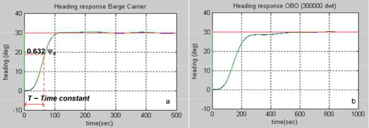
Simulation without disturbance is conducted on 20 types of ships with a set of heading point at 30o. The response of the control system shows stability. Response of Barge Carrier and OBO ships (300,000 DWT) is shown in Fig. 4. The response has the response pattern of the first order system [13]. Time constant of a system is a time when the response reaches 63.21% of the target. Response with second-order pattern system shown in Fig. 5 at River Tow Boat U.S. ship and Tuna Seiner.

The response of a system is expressed in first order (Fig. 4), with a parameter time constant (T) and gain (K). The smaller the value of T, the faster the system response will be, and vice versa, the larger the T, the longer the target heading will be reached. When t≥3T, response will be included in the region of 5% of the final condition or in the steady state condition [13]. If a system is said to have second order, the system will

received a step function input and will give response as shown in Fig. 5. The occurrence of overshoot and oscillation pattern in its steady conditions will subsequently reduce or even eliminate this oscillation. Characteristics shown in the Fig. at the time of the transient state are influenced by the amount of damping ratio ζ and frequency of natural ωn. Transfer function

form of second-order system expressed in equation (13) below: 2 2 2 ) ( ) ( n ns s K s R s C ω ζω + +

= (13)

with ζ: damping ratio of system, ωn : natural frequency

of system (Ogata, 1992).

Table 1 shows the specifications of length and speed of service from some ships investigated in this research. The order system is obtained from trajectory system response when given setting ship heading as a step function at 30o. Time constant system is the value of which the response system reaching 63.2% of the expected headings. Out of 20 types of ships, there are 16 which are mostly approached with first order system, while Harbor Tug boats, River Tow Boat U.S., Offshore Supply and Tuna Seiner are approached with the second order pattern. The time constant values of 20 types of ships range between 33.36 - 418.60 seconds as shown at Table 1. There are indications that this result is better than others (Wahl, 1998) that produce the time constant T = 56.2 seconds on the type of ship of length L = 80 meters.

Ship maneuvering system with inertia matrix M and damping matrix D is seen as a high order of systems, where higher order systems are approximated with second order system with parameter ω damping ratio, natural frequency of the system ωn, ζ and natural

frequency from system. Settling time (Ts) for parameter

value between 0 <ζ <0.9, can be obtained by determining the following equations [14].

(15)

Ts values obtained by calculation and simulation results

seen in appendix B. Comparison calculations with the simulation results obtain Ts error average in the determination of Ts and a small variance.

B. The Calculation of the Gain Control Value Nomoto and Parameter Norrbin

Nomoto (1957) has done ship maneuvering dynamics approach to show the form of mathematical order 1 and 2, with parameters as in table 1 [12]. Determining parameter in the control gain is derived based on the linearization of the model Nomoto Davidson and Schiff (1946), whereas the form of Nomoto gain control equation is as the following:

) det( 1 21 2 11 N b n b n

K= − (16)

with,

det (N) = (17)

det(M)= (18)

n11= −Y_v (19)

n21=−N_v (20)

b1=

(

)

(

)

) det( M

δ

δ mx Y N

Y N

I_z − _r& − _G − _r& (21)

b2 =

(

)

(

)

) det( M

δ

δ mx N Y

N Y

Based on the Nomoto equation that express in equation (16) above, the gain controller is calculated based on the coefficient of hydrodynamic Clarke (1982) and then compared with the output that has been mentioned in Table 1. From the table, it is described that the 16 types of ships are analyzed using system order 1, and then the 4 types of ships are analyzed using order 2. Determining the value of the control gain K based on the output response time of the simulation set point heading as a step function can be done through the calculation of the return inverse of the form Equation:

(1 ))

) (

) (

Ts s

K s

s

+ = δ ψ

with a value of T and Ts in Table 1 for order 1 system.

For the second-order system is done by the return inverse of the transfer function expressed in equation (13) with a damping ratio value ξ and the natural frequency system ωn which has been obtained from the results of previous

studies [15]. The results of this K value is stated in table 2.

Table 2. presents Norbin parameters calculation. That is used as one of the parameters that determines the maneuver ability. If the value of this parameter is bigger than 0.3, the ship’s controller will show a guarantee for good maneuverability. This parameter is obtained based on the value of the control gain K' (response) and a constant time constant T'. From the Norrbin parameter values, it can be seen that General Cargo Low Speed, Mariner, RO/RO and Barge Carrier have better maneuverability compared to the 16 types of ships.

V.CONCLUSION

From the analysis and discussion it can be concluded that:

1.The FLC design will optimally worked when the length of all types of ships ranges from 40-350 meters. 2. Nomoto Gain Value and Norbin Parameters can be

obtained based on the analysis of the control system performance.

3. The FLC control performance is able to produce the best maneuvers in Low Speed General Cargo ships.

REFERENCES

[1] Mirosław Tomera, 2009, “Nonlinear controller design of a ship autopilot”, Int. J. Appl. Math. Comput. Sci., 2010, Vol. 20, No. 2, pp. 271–280 DOI: 10.2478/v10006-010-0020-8

[2] Yaohua Hu, Suwu Xu, 2010, “Generalized predictive controller design for ship track keeping”, ICCSNS International Journal of Computer Science and Network Security, May, Vol 9. No. 5.

[3] Fossen, T.I, 1992, “Guidance and controehicle”, John Wiley and Sons, 1994, pp. 79–81.

[4] Lewis. E., 1989, “Priciples of naval architecture: second revision,. motion and waves and controllability”, The Society ofNaval Architecturs and Marine Engineers 601 Pavonia Avenue, Vol. III, pp. 27.

[5] Aisjah, A.S, et al, 2011, “Analisa performansi MCST- (Monitoring and Control in Sea Transportation) pada kondisi kepadatan lalu lintas pelayaran di Alur Barat Tanjung Perak, Proposal Penelitian Kompetitif ITS.

[6] Aisjah, A.S., Soegiono, Masroeri, AA., Djatmiko, E.B., Wasis dan Sutantra, I.N., 2004, “Tracking linier wahana laut berbasis logika fuzzy”, Seminar Nasional Pasca Sarjana ITS, Agustus. [7] Aisjah, A.S., Soegiono, Masroeri, AA., Djatmiko, E.B., Wasis ,

Sutantra, I.N dan Buda, K., 2005, “Pengembangan kontrol tracking wahana laut berbasis logika fuzzy”, Seminar Nasional Fakultas Teknologi Industri ITS, Maret.

[8] Aisjah, A.S., Soegiono, Masroeri, A.A., Djatmiko, E.B. ,Wasis, Sutantra I.N. dan Buda, K., 2005, “A study of extended fuzzy logic control for ship maneuvering based on LQG/LTR control”, Seminar Nasional Fakultas Teknologi Industri ITS, Maret. [9] Aisjah, A.S., Masroeri, AA., 2005 , “Maneuvering sea vehicle

using lqr control”, Proceeding Seminar Pasca Sarjana ITS, Agustus.

[10] Aisjah, A.S., Masroeri, A.A. 2005, “Extended fuzzy logic control for ship maneuvering based on LQG/LTR control”, International Seminar ISME – Japan, October.

[11] Aisjah, A.S., Soegiono, Masroeri, A.A., Djatmiko, E.B., Wasis, D.A, dan Sutantra, I.N , 2007, “Strategi kontrol robust LQG/LTR dalam mengatasi gangguan gelombang dan arus laut pada kapal”, Jurnal GEMATEK STIKOM Surabaya, Maret. [12] T.I Fossen, 1993, “High perfromance ship autopilot with wave

filter”, 10’th Ship Control System Symposium (SCSS), Cannada,. [13] K. Ogata, 1998. “Modern control engineering”, M.G Hill, [14] B. Kuo, 1995, “Otomatic control”, Mc. Graw Hill, pp. 278. [15] Aisjah, A.S, 2007, “Pengembangan sistem kontrol logika fuzzy

dengan model referensi kontrol LQG/LTR untuk membangun wahana tanpa awak”, Disertasi S3, Teknik Pengendalian Kelautan, FTK, ITS.

[16] Wen-Hsien Ho, Chen-Huei Hsieh and Jyh-Horng Chou, 2010, “Optimal course handling control for nonlinear ship maneuvering systems”, International Journal of Innovative Computing, Information and Control ICIC, International 2010 ISSN 1349-4198, October, Vol. 6, No. 10.

[17] Lozowicki, A.dan Tiano, A., 2000, “On the design of a high precission ship track keeping system”, 5th IFAC Conference on Maneuvering and Control of Marine Craft, MCMC 2000, Aalborg, Denmark.

[18] Nejim, S., 1998, “Design of limited authority adaptive ship steering autopilots”, IFAC Conference CAM’S 98, 27 – 30 October, Fukuoka Japan.

[19] Bertin, D., 1998, “Track Keeping Controller for a Precission Manoeuvring Autopilot”, IFAC Conference CAMS’98, Fukoka, Japan.

[20] Kijima, K. dan Murata, K., (1998), “Design of a Dynamic Positioning System for Self – Propulsive Barge under External Disturbances”, IFAC Conference CAM’s ’98, Fukuoka Japan. [21] Strand, M. F. , Jann, P., dan Fossen, TI., 1998, “Nonlinear

Vectorial Observer Backstepping with Integral Action and Wave filtering for Ships”, IFAC Conference CAM’S 98, Fukuoka Japan.

[22] Strand, M.F, Jann, P. dan Fossen, T. I., 1998, “Nonliear output feedback and Locally Optimal Control of Dynamically Positioned Ships : Experimental Results”, IFAC Conference CAM’S 98, Fukuoka Japan.

[23] Consegliere, A. dan Lopez, M.J., 2000, “H∞ Controller Tuning Method for Ship Autopilot”, 5th IFAC Conference on Manoeuverring and Control of Marine Craft, MCMC , Aalborg, Denmark.

[24] Omerdick, E., dan Roberts, G.N., 2004, “A fuzzy track – keeping autopilot for ship steering’, Journal of Marine Engineering and Technology, Vol. A2.

IPTEK, The Journal for Technology and Science, Vol. 21, No. 2, May 2010

Fig. 2. The development of ship maneuvering control system design

Fig. 4. Step response of ship in type of firts order (a) Barge Carrier (b) OBO (300 000 dwt)

Fig. 5. Step response of ship in type of firts order (a) US River Tow Boat , (b)Tuna Seiner

TABLE 1.

TYPE OF SHIP AND APPROXIMATION ORDER SYSTEM DETERMINATION AND THE CONSTANT TIME SYSTEM APPROACHES

Types of Ships Lpp

(m)

U (m/s)

Order System Approach

T (s)

T’ = T(U/L)

Settling Time (Ts)

FLC LQG/LT

R

Harbor Tug 43.26 5.15 2 42.21 5.03 104.8 113.6

US River Tow Boat 43.30 5.15 2 64.23 7.64 87.9 91.7

Offshore Supply 58.28 6.69 2 63.11 7.24 123.4 133.7

Tuna Seiner 72.03 8.23 2 39.94 4.56 108.0 121.2

Container High Speed 78.18 14.67 1 33.36 6.25 68.6 74.3

Car Ferry 93.56 10.29 1 46.6 5.12 73.7 95.1

Cargo Liners 141.78 10.81 1 90.82 6.92 143.7 158.9

Lumber Low Speed 152.04 7.72 1 155.73 7.90 247 265.4

General Cargo Low Speed 152.09 7.72 1 127.22 6.45 138.0 150.5

Mariner 161.90 7.72 1 107.89 5.14 118.7 131.3

RO/RO 193.59 11.32 1 116.51 6.81 216.0 241.8

Container Med. Speed 209.4 11.32 1 132.61 7.16 194.0 211.7

Tanker (Panamax) 237.65 7.72 1 277.45 9.01 439.0 444.1

OBO (Panamax) 239.74 8.24 1 295.14 10.14 467.0 475.9

Barge Carrier 244.03 9.78 1 178.1 7.13 339.4 352.5

LNG (125 000 m3_{) 270.11 10.29 1 217.87 8.30 186.5 202.0}

OBO (150 000 dwt) 270.39 7.72 1 301.19 8.60 473.7 483.11

Tanker 100 000 - 350 000 dwt 304.65 8.24 1 289.82 7.84 439.0 450.9

OBO (300 000 dwt) 310.40 7.72 1 345.07 8.58 545.8 591.3

Tanker 350 000 dwt 409.59 8.24 1 418.60 8.42 598.8 612.7

IPTEK, The Journal for Technology and Science, Vol. 21, No. 2, May 2010

TABLE 2.

GAIN CONTROL OF THE SHIP BASED ON SYSTEM RESPONSE AND BASED ON FIRST ORDER NOMOTO EQUATION AND THE COEFFICIENT NORRBIN

Types of Ships Control Gain (K)

Norbin Parameter 0.5(K’/T’)(L2_/U2₎

Response Calculation

Harbor Tug 0.19392 0.1810 1.36150

US River Tow Boat 0.17310 0.1660 0.80088

Offshore Supply 0.09425 0.1060 0.49367

Tuna Seiner 0.20400 0.2110 1.71212

Container High speed 0.14800 0.1220 0.33574

Car Ferry 0.21900 0.2010 1.76625

Cargo Liners 0.08400 0.0841 1.04339

Lumber Low Speed 0.04290 0.0491 1.05215

General Cargo Low Speed 0.13600 0.1190 4.08712

Mariner 0.18400 0.1850 7.86494

RO/RO 0.28500 0.2160 6.11721

Container Med. Speed 0.06500 0.0698 1.55133

OBO (Panamax) 0.01800 0.0280 1.10400

Tanker (Panamax) 0.02100 0.0161 0.75102

Barge Carrier 0.16800 0.1440 7.32704

LNG (125 000 m3 _{) 0.07990 0.0715 3.31665}

OBO (150 000 dwt) 0.02070 0.0197 1.47646

Tanker 100 000 - 350 000 dwt 0.02390 0.0202 2.08380

OBO (300 000 dwt) 0.01790 0.0173 1.68588