WHEN DOES INCOME INEQUALITY CAUSE POLARIZATION?
Jacob R. Gunderson
A thesis submitted to the faculty of the University of North Carolina at Chapel Hill in partial fulfillment of the requirements for the degree of Master of Arts in the Department of Political Science.
Chapel Hill 2019
Approved by:
Gary Marks
Evelyne Huber
ABSTRACT
Jacob R. Gunderson: When Does Income Inequality Cause Polarization? (Under the direction of Gary Marks)
ACKNOWLEDGEMENTS
TABLE OF CONTENTS
LIST OF TABLES . . . vii
LIST OF FIGURES . . . viii
1. INTRODUCTION . . . 1
2. MELTZER-RICHARD AND PARTY COMPETITION . . . 3
3. PARTISANSHIP AND ISSUE SALIENCE AS CRUCIAL CONTEXTUAL FACTORS . . . . 7
4. EMPIRICAL IMPLICATIONS . . . 10
5. DATA & MODEL SPECIFICATION . . . 12
5.1 Dependent Variable: Party Polarization . . . 12
5.2 Independent Variables . . . 14
5.3 Controls . . . 16
5.4 Models . . . 18
6. RESULTS . . . 20
6.1 Income Inequality’s Conditional Effect . . . 22
6.2 Beyond Meltzer-Richard . . . 24
7. DISCUSSION AND FUTURE RESEARCH . . . 27
8. APPENDIX . . . 30
8.1 Salience Categories . . . 30
8.3 Correlation Matrix for Variables in Models . . . 35
8.4 Checks of Model Fit for Multi-Level Model . . . 36
8.5 Models using Only CSES Data . . . 40
8.6 Models using other Measures of Income Differentiation . . . 41
8.7 Models with Single Interactions . . . 43
8.8 Models Using Only Data from Western Europe . . . 45
LIST OF TABLES
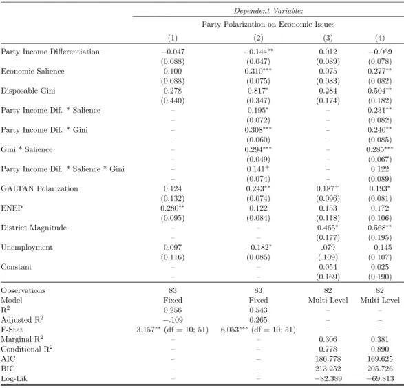
1 Results from Fixed Effects and Multi-Level Models . . . 21
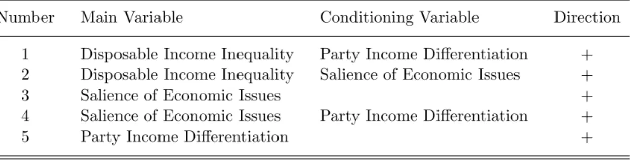
2 Summary of Hypotheses on Party Polarization on Economic Issues . . . 22
3 Components of Socio-Economic Salience . . . 30
4 Components of Socio-Economic Salience Cont. . . 31
5 Cases and Economic Polarization . . . 32
6 Income Differentiation, Disposable Income Inequality, and GALTAN Polar-ization by Country . . . 33
7 Economic Salience and Continuous Controls . . . 34
8 Correlations of Variables in Main Models . . . 35
9 Results from Fixed Effects and Multi-Level Models Using only CSES Data . . . 40
10 Fixed Effects Models using Alternative Income Dif. Measures . . . 41
11 Multi-Level Models using Alternative Income Dif. Measures . . . 42
12 Fixed Effects Models with Single Interactions . . . 43
13 Multi-Level Model with Single Interactions . . . 44
LIST OF FIGURES
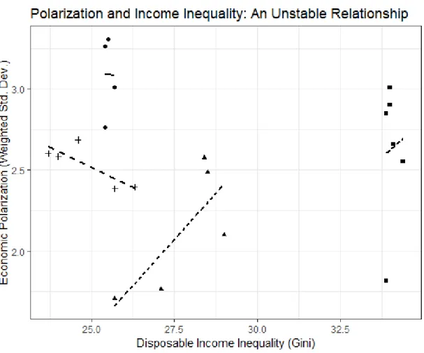
1 Expert Evaluations of Party Positions in Three Elections. . . 6
2 Chapel Hill Expert Survey Evaluations of Party Positions in Three Elections. . . 13
3 Marginal Effect of Disposable Income Inequality on Party Polarization . . . 23
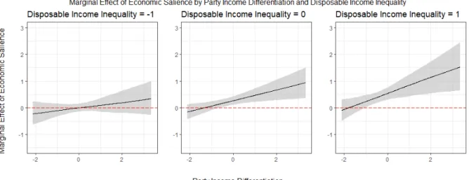
4 Marginal Effect of Disposable Income Inequality by Economic Salience . . . 24
5 Marginal Effect of Economic Salience on Party Polarization . . . 25
6 Marginal Effect of Party Income Differentiation on Party Polarization . . . 26
7 Observed vs. Predicted Values . . . 36
8 Observed vs. Predicted Values by Country . . . 37
9 Q-Q Plot . . . 38
1. INTRODUCTION
Although recent scholarship, particularly in the United States, focuses on political polarization in recent decades (or lack thereof) (Abramowitz and Saunders, 2008; Fiorina and Abrams, 2008; Fiorina, Abrams and Pope, 2011; Hetherington and Weiler, 2009), the study of polarization is hardly new. Giovanni Sartori’s seminal 1976 book, Parties and Party Systems, is one of the earliest works on this topic, and it clearly recognizes the stakes in understanding polarization’s origins and implications. Drawing principally on the Weimar Republic, Chile before 1973, and the French Fourth Republic, Sartori writes that in polarized party systems, “...cleavages are likely to be very deep, consensus is surely low, and the legitimacy of the political system is widely questioned”(Sartori, 1976, 120). Contemporary research often highlights implications that are potentially more positive, such as increased ideological voting (Lachat, 2008), lower electoral volatility (Dejaeghere and Dassonneville, 2017), and diminished support for anti-establishment parties (Abedi, 2002), but it remains clear that whether parties crowd together or stand near ideological poles has significant consequences for politics and society.
Given polarization’s effect on these important outcomes, it is vital to understand why party systems exhibit centripetal or centrifugal tendencies. One line of scholarship argues that parties should polarize on economic issues under conditions of high income inequality (Meltzer and Richard, 1981). When income inequality is high, parties of the left should be expected to campaign vigorously for redistribution while right-wing parties seek to defend their supporters’ wealth (Han, 2015; Winkler, 2019).
economic position and geographic location (Lipset and Rokkan, 1967). I argue the connection between income inequality and party positions depends on partisanship grounded in the economic position of party supporters. Where different parties in a party system cater to divergent economic bases, it makes sense for them to take extreme stances in the face of high income inequality. If this is not the case, parties taking extreme positions are much more likely to alienate their own partisans, so there is little incentive for parties to polarize.
The importance of economic issues in an election also has a substantial conditioning effect. Even in states with high income inequality and party bases constructed around economic positions, the salience of economic issues in national elections varies. When parties and voters deemphasize economic concerns in a given election relative to other points in time, there is less to be gained from staking out economic positions near the poles, so polarization should be lower than when an election revolves around the economy (Alvarez and Nagler, 2004). In elections dominated by economic concerns, parties are incentivized by their base and the focus of the campaign to stand apart from one another rather than cluster together.
2. MELTZER-RICHARD AND PARTY COMPETITION
Currently, there are two primary arguments that relate income inequality to the degree of party polarization. The first argues that a higher level of income inequality leads to more polarized party systems. The fundamental argument rests on the relationship between the mean income voter and the median income voter (Meltzer and Richard, 1981). Assuming that individual attitudes toward redistribution are the product of a voter’s position in the income distribution, the median voter will always stand to benefit from redistribution, and the intensity of this position should increase as the gap between the median and mean income expands (as the income distribution becomes less egalitarian)(Meltzer and Richard, 1981). If parties respond to this increase in income inequality strategically, then the expectation should be that parties in unequal societies, particularly in multi-party systems, will take extreme positions relative to parties in more equal societies in order to better represent and attract the support of voters. Therefore, party systems with higher levels of income inequality should have some parties far to the left and some parties far to the right, yielding a high degree of polarization.
Evidence from the United States appears to support this argument. McCarty, Poole and Rosenthal (2006) find that income inequality (Gini index) and polarization, measured as the difference between the average member of congress in each party using DW-Nominate scores, in the Unites States have moved in tandem with both increasing since the 1980s. Han (2015) finds evidence for this in a comparative framework, but he argues that this relationship only holds true in certain institutional settings. Specifically, he argues that we should see a positive relationship between income inequality and polarization only under permissive electoral systems, which he operationalizes as having a high district magnitude.1 In these systems, parties face less of an incentive to compete for the median voter, so parties are able to move further from the center when faced with higher levels of income inequality. Individual-level data regarding the probability of voting for extreme parties under different levels of income inequality also provides some support for the Meltzer-Richard
model’s application to polarization. Using regional inequality measures, Winkler (2019) finds that the probability of voting for a party of the radical left or radical right is positively related to regional income inequality.
Other scholars have attempted to modify Meltzer-Richard’s framework to better reflect the realities of contemporary party competition. Pontusson and Rueda (2008) deviate slightly from the Meltzer-Richard framework by considering two additional factors. First, they argue that different types of economic inequality matter to different types of people. As many workers with low incomes depend on wages as their primary source of funds, they should care about wage inequality (90/10 earnings ratio), but the relatively well-off voters that constitute the core constituency of the economic right should be more sensitive to household income inequality (operationalized as disposable household income as this includes sources of income beyond wages). Secondly, Pontusson and Rueda (2008) argue that it is important to consider the degree to which low-income voters are mobilized. Higher levels of income inequality may suppress electoral participation, particularly at the lower end of the income distribution (Anderson and Beramendi, 2008; Solt, 2008, 2010). Therefore, when income inequality is high, parties of the left may have to moderate their positions to maintain their vote share. Focusing only on the two largest parties in twelve OECD countries, Pontusson and Rueda (2008) find that when low-income mobilization is high, left-wing parties facing high income inequality take more leftist positions on economics than when income inequality is low. This establishes that income inequality may not always be positively correlated with extreme party positions depending on the strength of income inequality’s effect on turnout.2
Fenzl (2018) argues that income inequality’s effect on polarization, including all parties in a party system, will be negative. This is partly due to the effect of income inequality on electoral turnout, but also because under high levels of income inequality, right wing parties, which are less sensitive to income inequality’s effect on turnout, have little incentive to move to the extremes. This should be particularly true if the parties of the left moderate their positions. In such circumstances, a right-wing party moving to the extremes may lose their own moderate voters to a left-wing party moving to the center (Adams, 2001). In line with these expectations, Fenzl (2018) finds that income inequality has a negative effect on economic polarization.
2
Many scholars have argued that income inequality ought to have an effect on political polarization, but there is no consensus on what that effect is. Three recent studies on this subject using very similar data, come to contradictory conclusions (Han, 2015; Fenzl, 2018; Winkler, 2019).
Figure 1: Expert Evaluations of Party Positions in Three Elections.
3. PARTISANSHIP AND ISSUE SALIENCE AS CRUCIAL CONTEXTUAL FACTORS
Existing studies relating income inequality to political polarization operate under the assumption that political parties are sorted by income with low-income and workers forming the key constituency of the left and the middle-class and business owners forming the core constituency of the right. Historically, we know that the connection between income level and party choice should not be treated as a given (Marx, 2008; Rueschemeyer, Huber Stephens and Stephens, 1992). Even though an individual’s income might be below that of the median voter, they may be a partisan of the right because they oppose redistribution or because there is some other factor driving party selection like positions on other dimensions, social identities, or the charisma of individual politicians (Greene, 2004; Huddy, Bankert and Davies, 2018). Critically, the social construction of partisanship is absent in Meltzer-Richard’s framework, which assumes politically behavior is driven by economic rationality.
As Huber and Stephens (2012) argue, Power Resource theory does a better job of explaining real world outcomes than the Meltzer-Richard model because it acknowledges that an individual’s position in the distribution of income does not determine their ideological position or party choice. Having an income below the median does not predetermine ideological allegiance because class and the political priorities of the poor are socially constructed. This is clearly evident in the contrast between the rural and urban poor. The rural poor are more vulnerable to conservative cultural influence, and therefore frequently support conservative political causes (Rueschemeyer, Huber Stephens and Stephens, 1992). However, where organizations are able to construct a conception of class as being grounded in the conflict between the haves and have-nots, which is easier in urban centers where large masses of workers live in close proximity, political movements are likelier to support redistribution.
income differences between partisan groups is high. This incentive should be greater when income inequality is high. In other words, I expect income inequality to have the effect Meltzer and Richard (1981) predicts only when partisanship runs along economic lines.
My argument rests on the connection between the degree to which partisans are clearly differenti-ated with respect to income and the salience of conflict over economic issues. Group differentiation’s effect on conflict has found support in other fields of political science, particularly in the study of civil conflict (Stewart, 2008, 2016; Cederman, Weidmann and Gleditsch, 2011). In this context, there are robust findings that the probability of conflict onset increases when horizontal inequality (the degree of inequality between groups) is high. This informs the debate in the conflict literature related to the contribution of grievances to conflict, which has often taken the form of economic grievances (Fearon and Laitin, 2003). Overall inequality in a society does not appear at first to have any robust role in predicting conflict because the important thing for conflict is how resources are distributed between groups, not just across society at large.
Of course, there are many potential ways of dividing a society. For the purpose of this paper, I argue that political parties represent relevant groups. This is appropriate given that my theory relies on the connection between the economic position of voters and their membership in parties. Additionally, Huddy, Bankert and Davies (2018) finds that the social identity approach to partisanship functions in the context of European party systems, so party supporters likely view themselves as distinct groups. Parties do, however, represent a more fluid type of identification than racial or religious identities, but given that partisan identity is a strong, negative predictor of vote switching (Dejaeghere and Dassonneville, 2017), I believe that parties are cohesive enough to represent meaningful groups for the purposes of this paper.
if parties are highly differentiated with respect to the income of their supporters but the groups of supporters are not that divergent from one another (for example the upper middle class vs. lower middle class), then I would expect party polarization to be lower than when the groups of supporters are highly divergent (bottom 10% vs. top 1%). Oskarson (2005) shows some evidence for this connection. Using a measure of class voting, she finds that class voting is positively related to the total span of parties on a number of dimensions. Evans, Heath and Payne (1999) investigate a similar question in the context of the UK. Again, it appears that the social distribution of voters between parties has an effect on party polarization.
4. EMPIRICAL IMPLICATIONS
The theoretical argument outlined above implies several empirical relationships that establish the importance of party income differentiation and the salience of economic issues as critical contextual factors that moderate the effect of income inequality on party polarization. Under the standard Meltzer-Richard framework, the principal expectation is a positive relationship between income inequality and party polarization. My argument, however, suggests that the positive relationship is stronger, if present at all, when parties themselves are sorted by income. If parties are not differentiated by income, then the situation is akin to party system B above, and little relationship should exist.
H1: There will be a stronger positive relationship between income inequality and party polarization on economic issues when partisan income differentiation is high.
In addition to the level of partisan income differentiation, the salience of economic issues should also condition the translation of income inequality into polarization. Not all elections emphasize economic issues to the same extent, even in countries where parties are clearly sorted with respect to income. Much like H1, a stronger, positive relationship between income inequality and polarization when the salience of economic issues is high would provide support my argument that Meltzer and Richard (1981)’s model translates to party politics only when the political context is taken into account.
H2: There will be a stronger, positive relationship between income inequality and party polariza-tion on economic issues when the salience of economic issues is high.
low, even a party system with high levels of partisan income differentiation and income inequality may not be that polarized, but where the salience of economic issues is high, I expect party systems with high levels of income inequality and partisan income differentiation, like party system A above, to be more polarized than a party system with a lower level (like party system B).3 This argument is reflected in the following hypotheses:
H3: The level of economic salience will have a positive relationship with the level of polarization on the economic left-right dimension.
H4: The salience of economic issues will have a stronger association with party polarization on economic issues when the degree of partisan income differentiation is high.
Finally, I expect higher levels of partisan income differentiation to have a positive relationship with party polarization. Where parties’ bases grow apart, which may be the result of factors beyond those pertinent to the Meltzer-Richard framework, parties should have an incentive to respond by pulling apart from each other in ideological space.
H5: The degree of partisan income differentiation will be positively associated with the level of polarization on the economic left-right dimension.
In the following sections, I discuss the data, operationalizations, and models that I use to test these hypotheses.
3It could be argued that income differentiation and economic salience are endogenous to one another. Empirically,
5. DATA & MODEL SPECIFICATION
5.1 Dependent Variable: Party Polarization
The dependent variable of this study is party polarization, which I define as the degree to which parties take positions far from the political center in an election. In particular, I draw on Sartori (1976) to highlight two key facets of polarization: the distances between parties and the, “... enfeeblement of the centre, a persistent loss of votes to one of the extreme ends (or even to both)” (Sartori, 1976, 120, italics original). In this framework, large distances between parties in ideological space indicate more disagreement between parties. The vote share received by each party reflects the centrifugal tendency Sartori (1976) discusses. Incorporating a party’s support is also important because it prevents small fringe parties from drastically increasing polarization. For example, considering the NPD, a fringe radical right party that receives a very small vote share, equivalent in the calculation of polarization in the German party system to theCDU, a large Christian Democratic party, would not reflect the reality of the party system. Weighting parties by vote share solves this problem.
I operationalize party polarization as the standard deviation of parties’ positions on a given dimension of contestation weighted by their vote share (Kim, Powell and Fording, 2010).4 I take party positions on economic issues from the Chapel Hill Expert Survey (CHES) (Bakker et al., 2015; Polk et al., 2017). This data source uses expert surveys to place political parties on a number of issue dimensions in European national elections. This study uses data from 22 countries from 1996 to 2016 for a total of 82 national elections.5 Expert surveys have several advantageous features. One is that experts are able to take into account both what parties say they are going to do and what they actually do in assessing a party’s position on a given issue dimension. This increases the validity of
4
Polarization is a contested concept, and as such there are many ways to operationalize it. Dalton (2008)’s polarization index is used or approximated by Han (2015) and Fenzl (2018). My operationalization of polarization has correlation of 0.978 when the same data are used to calculate Dalton’s index.
5
expert positions as they have more observations on which to draw when positioning parties than other estimates of party positions that depend on a single data source. Additionally, because experts directly place parties on a quantitative scale, the method of aggregation is less problematic than in other methodologies (Gemenis, 2013). It is also possible to evaluate the agreement between experts in terms of party placement. In the case of the CHES, such validation indicates a high degree of inter-expert agreement (Marks et al., 2007; Steenbergen and Marks, 2007).
Figure 2: Chapel Hill Expert Survey Evaluations of Party Positions in Three Elections.
low level of polarization (.342, the lowest in the sample). Here, the largest parties are all centrally located and close to one another.6
5.2 Independent Variables
My first independent variable of interest is the degree of income differentiation between partisan groups in an election. I draw on research in international relations and development to operationalize the inequality or differentiation between partisans (Østby, 2008; Cederman, Weidmann and Gleditsch, 2011; Gubler and Selway, 2012). Stewart, Brown and Mancini (2010) provide a useful discussion of intergroup inequality measures. These measures seek to satisfy the following four axioms:
1. Independence of the distribution from the mean,
2. The principle of transfers (Pigou-Dalton): transfers from a richer person (group) to a poorer person (group) reduces inequality,
3. In so far as possible, to find a measure which is descriptive, not evaluative. This is not perfectly achievable since any measure involves some implicit valuation, but we aim to minimize this and hence will discard measures which have explicit inequality aversion built in, and
4. To measure group inequality as such, not the contribution of group inequality to either social welfare as a whole (like the gender-weighted Human Development Index (HDI)) or to income distribution as a whole (Stewart, 2008, 87)
The first two of these are borrowed from standard calculations of inequality for an entire society (often called vertical inequality).7 The latter two are specific to horizontal inequality measures. In keeping with these four axioms, I use the following equation for the group Gini coefficient (Stewart, 2008):
GGIN I = 1 2¯y
R X
r S X
s
prps|y¯r−y¯s| (1)
6Table 5 in the appendix displays the countries in my sample with complete data for all analyses, the number of
elections I have for each country, the earliest and most recent election, the mean polarization for each country on each dimension, and the standard deviation of polarization for each country.
7Metrics of vertical inequality typically also seek to satisfy an additional criteria: “The transfer of an equal amount
For my purpose, ¯y is the overall mean income, R and S are counters of the total number of parties in a party system, ¯yr is the mean income of partyr, ¯ys is the mean income of party s, and
pr and ps are party r and party s’ share of partisans. This measure essentially determines the absolute value of the pairwise differences in mean income between all parties in the system weighted by the proportion of partisans in each party dyad. Then, these absolute differences are summed and multiplied by a standardizing coefficient.8 I determine ¯y, ¯yr, and ¯ys using the mean reported income quintile of party members from the Comparative Study of Electoral Systems (CSES) and the European Social Survey (ESS). Both studies include items asking individuals to place themselves in income categories and which party, if any, they feel close to. I require two data sources as neither completely covers the cases in the CHES. In order to combine the two data sources and account for any systematic differences that may be present, I use a model to predict the level of partisan income differentiation in the CSES data using the ESS data. I then use this model to predict five sets of plausible values for partisan income differentiation, run my models five times with a different set of plausible values in each iteration, and then average the results from all five models together.9 I operationalize income inequality using data from the Standardized World Income Inequality Database (SWIID) (Solt, 2016). One of the major difficulties in cross-national research using measures of income inequality is comparability, as many data sources rely on different definitions of income inequality. The Luxembourg Income Study (LIS) is the gold standard of income inequality data in this respect because it harmonizes data from national data sources. However, LIS gathers data in waves, not annually, so using only LIS data would result in a very low number of cases even in Western Europe. SWIID uses LIS data as a benchmark against which to standardize income data from a number of other sources. This source is ideal for my tests as it expands the number of
8
In addition to the group Gini coefficient, a group covariance and group Theil index are also proposed. There are differences between these measures (see Stewart, Brown and Mancini (2010) for more detail), but they are correlated by design. Because the notion of income differentiation is somewhat analogous to a form of party income polarization, I also construct the standard deviation of party mean incomes weighted by party membership as an additional robustness check. Results from models using these alternative operationalizations are presented in the Table 10 and Table 11, and they do not yield substantively different results.
9
possible observations by providing data annually, including data for countries not participating in LIS waves. Specifically, because I am interested in the way partisan divides are constructed along economic lines, I focus on income inequality after taxes and transfers (disposable income inequality). Redistribution and taxes can play a substantial role in determining the income level of individuals and the distribution of resources within a society, so income inequality measured based on income levels after taxes and transfers gives a better indication of the economic reality faced by individuals than before tax and transfer measures. Pensioners are a particularly good example of this. Because they do not generate market income, measures of wage inequality interpret retirees as without any income when they may be receiving government transfers, so disposable income inequality, which incorporates the effect of taxes and transfers, better models the economic realities for these voters and society overall.10
I argue that there should be more party polarization when economic issues are important in a national election. I operationalize the salience of economic issues in national elections from the Comparative Manifesto Project using Stoll (2010)’s socioeconomic salience category. Instead of focusing on the balance of positive and negative mentions related to a given issue or set of issues, I use the sum of quasi-sentences relating to economic issues divided by the total number of quasi-sentences in each party’s manifesto, essentially the proportion of the manifesto devoted to economic issues (Lowe et al., 2011). I then take the average for all parties in a given election year to determine the mean proportion of quasi-sentences devoted to economic issues.11 I list the relevant categories in the CMP data in the appendix.
5.3 Controls
I also consider potential alternative explanations for varying levels of polarization. One such explanation is the increasingly multi-dimensional political space in Western Europe (Stoll, 2010). The economic left-right division has been critical to politics since the industrial revolution, which is often treated as a critical juncture in the development of party systems (Lipset and Rokkan,
10
The mean and standard deviation of disposable income inequality and partisan differentiation (normalized to have mean 0 and standard deviation one) between parties with regards to income are presented in Table 6.
11
1967). The GALTAN dimension is a more recent development that is often linked to the rise of post-modern value systems, the increasing influence of the European Union on the lives of European citizens, and increased immigration flows from North Africa and the Middle East (Hooghe and Marks, 2009, 2018).12 There is the possibility that polarization on one dimension will influence polarization on the other. Because I am interested in polarization on economic issues here, I include polarization on the GALTAN dimension as a control variable.
In addition to the hypotheses above, I also acknowledge that there are institutional factors that likely play a strong role in the degree to which parties are able to polarize. I agree with Han (2015) that permissive electoral systems should lead to more polarized party systems because they do not induce political parties to compete for the median voter to the same extent as in a plurality system. Following Han (2015), I operationalize the permissiveness of the electoral system using the log of the average district magnitude. This variable is omitted from fixed effects models as it is constant for all but four of my cases.13 I also include the effective number of electoral parties (ENEP), anticipating that more parties in a system, particularly new, single issue, or extreme parties, will likely lead to higher overall levels of polarization. I take these variables from the Democratic Systems around the World Dataset (Bormann and Golder, 2013), which contains data from 1946 to 2016. Summary statistics of my salience measures and controls are presented in Table 7, which is located in the appendix.
Finally, I include a measure of the objective economic performance as a control. Han (2015) and Fenzl (2018) both include such measures in their analyses, although their results disagree on their significance. Due to my relatively small number of cases, I only include a single such variable, the unemployment rate, drawn from the Comparative Political Dataset (Armingeon et al., 2018).
12
This cleavage has alternatively been called the libertarian-authoritarian dimension (Kitschelt, 1995), cosmopolitan-parochialism (Inglehart, 1977; De Vries, 2017), and demarcation-integration (Kriesi et al., 2006).
13
5.4 Models
Because my data are repeated observations of European countries (each case is one country-election), I have time-series cross-sectional data comprised of eighty-two complete observations with twenty-two countries for an average of just under four observations per country. As stated above, the relationship between income inequality and party polarization on economic issues varies both between countries and within countries. I use a fixed effects model with panel corrected standard errors by country to isolate the within country effects from the cross-sectional variation (Beck and Katz, 1995).14 One shortcoming of the fixed effect approach is that institutional variables that are constant within countries but vary between countries are dropped. These variables include much of the institutional context, such as the electoral system. To overcome this difficulty and gain leverage on cross-sectional variation, I also fit the following multilevel model with a country random effects incorporating country-level institutions (Gelman and Hill, 2007):
P olarizationi ∼N(β0+αcCountryi
+β1IncomeDifi
+β2Saliencei
+β3Ginii
+β5IncomeDifi∗Saliencei +β6IncomeDifi∗Ginii
+β7Saliencei∗Ginii
+β8IncomeDifi∗Saliencei∗Ginii
+βcontrolsXControls+i,t, σ2P olarizationI) αc=γ0+γ1ElectoralInstituionc+ηc
(2)
where iis a country-election in the set of all elections, I,cis a country in the set of all countries,
C, andtindicates the election year.15 Because my theory suggests interactions between partisan income differentiation and disposable income inequality, between economic salience and disposable
14
I estimate this model using the plm command in the plm package inRusing the ’within’ setting (Croissant and
Millo, 2019).
15
income inequality, and between partisan income differentiation and the salience of economic issues, I also must include an interaction including all three terms (Braumoeller, 2004). Without including this interaction of all three variables, I would be implicitly assuming that a joint increase in partisan income differentiation, economic salience, and disposable income inequality has no relationship with party polarization on economic issues, an assumption which my theory does not indicate and my results do not strongly support.
An additional concern with time-series cross-section data is auto-correlation of observations for the same country across time. A Lagrange multiplier test and Wooldridge’s test for serial correlation in fixed effects panels both fail to indicate significant evidence of serial correlation in the fixed effects models. Additionally, I fit two versions of the multi-level model, one with and one without a first-order autocorrelation structure. The results from both models were very similar, and a likelihood ratio test failed to indicate that the model with first-order autocorrelation structure was a significantly better fit to the data than the simpler model.
6. RESULTS
In the previous sections, I argue that the effect of income inequality on party polarization should be contingent on the degree of partisan income differentiation in the party system and the importance of economic issues in the election. The results of the models outlined in Section Four are presented in Table 1. Models 1 and 3 omit any interactions between income inequality, partisan income differentiation, and the salience of economic issues. Models 2 and 4 include these interactions. Models 1 and 2 include country level fixed effects (omitted from Table 1). Models 3 and 4 are multi-level models with country-level random intercepts. Because the multi-level model does not eliminate cross-sectional variation as the fixed effects model does, I include the logged average district magnitude, which has also been scaled to have mean 0 and a standard deviation 1.
Model fit statistics confirm in both cases that the model including the interactions is a substan-tially better fit to the data than the restricted models. In the fixed effect models, the adjusted R2 is substantially higher in model 2 than model 1. This is noteworthy as the adjusted R2 calculation includes a penalty against the addition of variables, so model 2 improves the fit of the model despite the addition of four more predictors in a model already including a substantial number of predictors relative to the sample size.
There is a similar result in the multi-level model with the full set of predictors, which explain a higher percentage of the variance and have superior model fit statistics. The marginal R2 indicates the percentage of observed variation explained without the country-level intercepts, but the conditional R2 includes the country-level intercepts.16 In both cases, model 4 explains more of the variance than model 3. Model 4 also performs better with respect to the Akaike information criterion (AIC) and the Bayesian information criterion (BIC) (lower value indicates better fit) and the negative log-likelihood (higher value indicates better fit). Again, the AIC and BIC penalize less parsimonious models, so model 4 outperforms model 3 despite including more predictors.
16I calculated these statistics using the MuMin package inR, which calculates the statistics based on Nakagawa and
Table 1: Results from Fixed Effects and Multi-Level Models
Dependent Variable:
Party Polarization on Economic Issues
(1) (2) (3) (4)
Party Income Differentiation −0.047 −0.144∗∗ 0.012 −0.069
(0.088) (0.047) (0.089) (0.078)
Economic Salience 0.100 0.310∗∗∗ 0.075 0.277∗∗
(0.088) (0.075) (0.083) (0.082)
Disposable Gini 0.278 0.817∗ 0.284 0.504∗∗
(0.440) (0.347) (0.174) (0.182)
Party Income Dif. * Salience – 0.195∗ – 0.231∗∗
– (0.072) – (0.082)
Party Income Dif. * Gini – 0.308∗∗∗ – 0.240∗∗
– (0.060) – (0.085)
Gini * Salience – 0.294∗∗∗ – 0.285∗∗∗
– (0.049) – (0.067)
Party Income Dif. * Salience * Gini – 0.141+ – 0.122
– (0.074) – (0.089)
GALTAN Polarization 0.124 0.243∗∗ 0.187+ 0.193∗
(0.132) (0.074) (0.096) (0.081)
ENEP 0.280∗∗ 0.122 0.153 0.172
(0.095) (0.084) (0.118) (0.106)
District Magnitude – – 0.465∗ 0.568∗∗
– – (0.177) (0.195)
Unemployment 0.097 −0.182∗ .079 −0.145
(0.116) (0.085) (.109) (0.107)
Constant – – 0.054 0.025
– – (0.169) (0.190)
Observations 83 83 82 82
Model Fixed Fixed Multi-Level Multi-Level
R2 0.256 0.543 – –
Adjusted R2 −.109 0.265 – –
F-Stat 3.157∗∗(df = 10; 51) 6.053∗∗∗(df = 10; 51) – –
Marginal R2 – – 0.306 0.381
Conditional R2 – – 0.778 0.890
AIC – – 186.778 169.625
BIC – – 213.252 205.726
Log-Lik – – −82.389 −69.813
Turning to my hypotheses (displayed in Table 2), the results presented in Table 1 generally support my argument, but because my preferred models (2 and 4) include several interactions, the interpretability of individual coefficients is limited as the main effects of income inequality, partisan income differentiation, and the salience of economic issues represent the marginal effects of these variables when all other variables with which it interacts are held at their means. Additionally, because a three-way interaction is included, it is not possible to present the effects of my variables of interest in a single marginal effect plot. To display more meaningful representations of the results, I present figures containing panels of three marginal effect plots. In each of these figures, the effect of the variable of interest is the y-axis, the x-axis is the variable expected to interact with variable of interest, and the third variable is fixed at a constant value in each panel of the figure. As continuous variables are scaled with mean zero and standard deviation one, I fix the constant value at one standard deviation below the mean in the leftmost panel, the mean in the middle panel, and one standard deviation above the mean in the rightmost panel. As my hypotheses do not specifically apply to only within-country or cross-sectional variation, the following plots are based on the multi-level model. Table 12 and Table 13 in the appendix present fixed effects and multi-level models with each model containing only a single of the interactions. The results are robust but slightly weaker, except the interaction between party income differentiation and the salience of economic issues, which is in the right direction but not significant.
Table 2: Summary of Hypotheses on Party Polarization on Economic Issues
Number Main Variable Conditioning Variable Direction
1 Disposable Income Inequality Party Income Differentiation + 2 Disposable Income Inequality Salience of Economic Issues +
3 Salience of Economic Issues +
4 Salience of Economic Issues Party Income Differentiation +
5 Party Income Differentiation +
6.1 Income Inequality’s Conditional Effect
polarization on economic issues. Figure 3 depicts the marginal effect of disposable income inequality on party polarization with party income differentiation varying from its observed minimum to its observed maximum along the x-axis. In all three panels, the marginal effect of disposable income inequality increases with party income differentiation. Critically, this positive slope lifts the marginal effect from statistical insignificance in every panel when party income differentiation is very low to significant and positive as partisan income differentiation increases. This result supportsH1 and the larger theoretical point that the nature of partisanship in a party system conditions when income inequality translates into party polarization.
Figure 3: Marginal Effect of Disposable Income Inequality on Party Polarization
manifestos), even an above average level of party income differentiation does not yield a statistically significant effect of disposable income inequality on party polarization.
Figure 4: Marginal Effect of Disposable Income Inequality by Economic Salience
Together, these two results provide strong support for the theoretical contribution of this paper. Only when partisanship is constructed in such a way as to segregate individuals of different income levels into different parties and when economic issues are critical in elections, income inequality has the positive relationship with party polarization that the Meltzer-Richard framework postulates. This makes sense because in these cases reality approaches the underlying assumptions made in the model itself. Where parties are not clearly differentiated by income and economic issues are less critical, however, income inequality has no discernible effect.
6.2 Beyond Meltzer-Richard
is positive. There is also some conditionality here. When disposable income inequality is one standard deviation below its mean (a Gini coefficient of about 25.7, about the mean Gini coefficient of Slovakia), the salience of economic issues is never statistically distinguishable from zero. However, as income inequality increases, so does the proportion of covariate space in which the effect of economic salience is significantly greater than zero. This result provides support forH3.
Figure 5: Marginal Effect of Economic Salience on Party Polarization
Figure 5 also provides support for H4, which states that the effect of economic salience should be stronger in party systems where parties are more differentiable by the mean income of their partisans. The slopes of the marginal effects, particularly in the center and rightmost panel, support my argument. Looking at the middle panel, moving party income differentiation from one standard deviation below its mean to one standard deviation above its mean is associated with a change in the marginal effect of economic salience from essentially zero to about .5, so at that level, a one standard deviation increase in the proportion of manifesto quasi-sentences about economic issues (an increase of about 7%) is associated with a half standard deviation increase in the level of party polarization. This effect is even stronger in the rightmost panel when disposable income inequality is one standard deviation above its mean.
of disposable income inequality and the salience of economic issues, the effect of partisan income differentiation is significantly below zero or not distinguishable from zero.17
Figure 6: Marginal Effect of Party Income Differentiation on Party Polarization
The hypothesized positive effect is significant only when disposable income inequality is well above its mean and the salience of economic issues is about half a standard deviation above its mean. For context, this is the equivalent of economic issues taking up 49 percent of quasi-sentences in election manifestos and an after tax and transfer Gini coefficient of about 0.31, approximately the average level of disposable income inequality in Poland. This positive finding, then, offers partial support for H5. I return to this finding in the conclusion.
17Notably, the bivariate correlation between income differentiation is positive and statistically significant. See Table
7. DISCUSSION AND FUTURE RESEARCH
Income inequality and party polarization are two of the most important concepts for understand-ing the politics of developed democracies. The period of egalitarian economic growth followunderstand-ing the second world war has subsided, and income inequality has begun to grow to levels not experienced in nearly a century (Piketty, 2014). Time-series analysis has linked this increase in income inequality to increased party polarization in the United States (McCarty, Poole and Rosenthal, 2006), and there is some evidence for this in European democracies (Pontusson and Rueda, 2008; Han, 2015; Winkler, 2019). These findings fit with the Meltzer and Richard (1981) theory of political competition. As income inequality increases, we expect parties to respond to the divergence in income by taking positions that reflect the desperation of the poor for redistribution and the rich’s preference for maintaining their wealth.
This paper enriches previous research by arguing that the positive association between income inequality and party polarization is contingent on the construction of partisanship and the importance of economic issues in a national election. Using nationally representative and expert survey data for eighty-two European elections from 1996 to 2016, I find strong evidence for the relevance of these factors. When partisanship is unrelated to economic position or economic issues are not important in the election, income inequality has minimal effects. When parties have divergent economic bases and economic issues are crucial in an election, parties are likely to take highly polarized positions on economic issues. These contextual variables, particularly the importance of the economy in an election, also have their own significant relationships with the degree of party polarization.
early twentieth century. Where parties do not highlight the economic aspects of these issues and partisan bases are not built along economic lines, my results indicate that even a high level of income inequality will not lead parties to take positions that reflect the economic realities of families in their societies.
The results of this study suggest several promising avenues of future research. First, the salience of economic issues is a significant and substantive moderator of income inequality’s effect, but in many cases, issues that have economic implications may be framed in terms of identity or community values. For example, European integration has a clear economic impact on the citizens of member states. However, much of the resistance to an ever closer union is articulated through appeals to nationalism. The same can be said of issues relating to the movement of people both within Europe and into Europe from its neighbors. There are arguments to be made regarding its economic impact, but the issue is often treated as being as much about a confrontation of cultures and identities as a matter of economic rationality. Similar points also apply to welfare chauvinism (Oesch, 2008). The potential for such a connection is suggested by the significantly positive effect of GALTAN polarization on economic polarization in both of my interactive models. Further research into the framing of such issues should be carried out to determine how the colors with which an issue is painted effect the responses by voters and parties, particularly under conditions of steep income inequality.
the Alternative for Germany (AFD) became the third largest parties in their respective parliaments in 2018.
Rooduijn and Burgoon (2018) find that the poor are more likely to support radical parties under conditions of high income inequality, but whether they vote for the radical right or left seems to depend on additional contextual factors. When the economy is strong, income inequality appears to push poor voters to the radical right, but the probability that poor voters go to the radical left increase when the net flow of immigrants is low. Winkler (2019) finds similar results but finds significant cohort effects with older voters more likely to turn to the radical right than left.
8. APPENDIX
8.1 Salience Categories
Table 3: Components of Socio-Economic Salience
Name Label Description
per401 Free Market Economy Favourable mentions of the free market and free market capitalism as an economic model.
per402 Incentives: Positive Favourable mentions of supply side oriented economic policies (assistance to businesses rather than consumers).
per403 Market Regulation Support for policies designed to create a fair and open eco-nomic market.
per404 Economic Planning Favourable mentions of long-standing economic planning by the government.
per406 Protectionism: Positive Favourable mentions of extending or maintaining the protec-tion of internal markets (by the manifesto or other countries). per407 Protectionism: Negative Support for the concept of free trade and open markets.
Call for abolishing all means of market protection (in the manifesto or any other country).
per408 Economic Goals Broad and general economic goals that are not mentioned in relation to any other category. General economic statements that fail to include any specific goal.
per409 Keynesian Demand Manage-ment
Favourable mentions of demand side oriented economic poli-cies (assistance to consumers rather than businesses). per410 Economic Growth: Positive The paradigm of economic growth.
per411 Technology and Infrastructure: Positive
Importance of modernisation of industry and updated meth-ods of transport and communication.
Table 4: Components of Socio-Economic Salience Cont.
Name Label Description
per413 Nationalization Favourable mentions of government ownership of industries, either partial or complete; calls for keeping nationalised industries in state hand or nationalising currently private industries. May also include favourable mentions of govern-ment ownership of land.
per414 Economic Orthodoxy Need for economically healthy government policy making. per415 Marxist Analysis Positive references to Marxist-Leninist ideology and specific
use of Marxist-Leninist terminology by the manifesto party (typically but not necessary by communist parties).
per503 Equality: Positive Concept of social justice and the need for fair treatment of all people.
per504 Welfare State Expansion Favourable mentions of need to introduce, maintain or expand any public social service or social security scheme.
per505 Welfare State Limitation Limiting state expenditures on social services or social secu-rity. Favourable mentions of the social subsidiary principle (i.e. private care before state care) .
per506 Education Expansion Need to expand and/or improve educational provision at all levels.
per507 Education Limitation Limiting state expenditure on education.
per701 Labour Groups: Positive Favourable references to all labour groups, the working class, and unemployed workers in general. Support for trade unions and calls for the good treatment of all employees.
per702 Labour Groups: Negative Negative references to labour groups and trade unions. May focus specifically on the danger of unions abusing power. per703 Agriculture and Farmers:
Pos-itive
8.2 Variable Summary Statistics
Table 5: Cases and Economic Polarization
Economic Polarization Country # of Elections Earliest Latest Mean Standard Deviation
Austria 4 2002 2013 2.28 0.21
Belgium 3 1999 2010 2.41 0.13
Czech Republic 4 2002 2013 3.09 0.25
Denmark 5 1998 2011 2.28 0.21
Estonia 3 2007 2015 2.51 0.25
Finland 3 2003 2011 2.05 0.12
France 3 2002 2012 1.89 0.30
Germany 5 1998 2013 2.13 0.40
Great Britain 5 1997 2015 2.02 0.33
Greece 6 2004 2015 2.82 0.41
Hungary 3 2002 2014 0.57 0.20
Ireland 3 2002 2011 2.09 0.31
Italy 3 2001 2013 2.29 0.14
Lithuania 1 2012 2012 1.84 –
Netherlands 5 1998 2012 2.39 0.32
Poland 4 2001 2011 2.26 0.53
Portugal 5 2002 2015 2.79 0.19
Romania 1 2004 2004 2.33 –
Slovakia 3 2006 2012 2.62 0.11
Slovenia 2 2004 2008 1.38 0.25
Spain 6 1996 2016 2.51 0.46
Table 6: Income Differentiation, Disposable Income Inequality, and GALTAN Polarization by Country
Income Differentiation Disposable Income Inequality GALTAN Polarization
Country Mean Std. Dev Mean Std. Dev Mean Std. Dev
Austria -0.524 0.204 27.550 0.520 3.055 0.369
Belgium 0.063 0.266 26.367 0.493 2.521 0.134
Czech Republic 1.471 0.624 25.500 0.141 1.719 0.255
Denmark -0.095 0.542 23.800 1.070 2.058 0.363
Estonia 0.400 0.511 32.733 0.651 2.032 0.564
Finland 0.083 0.658 25.500 0.400 2.155 0.754
France -0.266 0.505 28.967 0.961 2.702 0.154
Germany -0.972 0.900 27.740 1.339 2.003 0.247
Great Britain -0.528 0.704 33.700 0.474 2.169 0.400
Greece 1.143 2.033 33.400 0.623 3.034 0.480
Hungary -1.046 0.222 28.167 1.026 2.965 0.214
Ireland -1.084 1.527 30.267 0.451 1.754 0.110
Italy 0.081 0.934 33.067 0.577 2.701 0.319
Lithuania -0.260 33.600 2.172
Netherlands 0.385 0.632 25.800 0.652 2.032 0.246
Poland 0.489 0.308 31.650 0.819 3.176 0.504
Portugal -0.873 0.464 34.080 0.192 2.698 0.463
Romania 0.331 32.300 2.053
Slovakia 0.055 0.376 25.633 0.379 1.941 0.203
Slovenia -0.498 1.038 23.450 0.212 2.919 0.333
Spain -0.584 0.943 33.050 0.855 3.103 0.777
Table 7: Economic Salience and Continuous Controls
Econ. Salience ENEP Dist. Mag. Unemployment
Country Mean Std. Dev. Mean Std. Dev. Mean Std. Dev. Mean Std. Dev.
Austria 45.885 3.336 4.167 0.979 4.260 0.000 4.800 0.648
Belgium 41.356 3.260 9.723 0.775 11.593 3.545 8.300 0.100
Czech Republic 47.451 5.460 5.761 1.688 14.290 0.000 7.175 0.150
Denmark 42.654 10.148 5.150 0.440 10.164 3.045 5.120 1.452
Estonia 48.784 0.980 4.963 0.211 8.420 0.000 7.700 4.063
Finland 56.976 1.905 5.997 0.417 13.300 0.000 7.900 1.054
France 45.536 8.307 4.923 0.522 1.000 0.000 8.567 1.069
Germany 46.043 1.771 4.400 0.701 1.000 0.000 8.400 2.223
Great Britain 40.894 6.807 3.554 0.289 1.000 0.000 5.940 1.303
Greece 44.751 3.497 4.599 1.826 4.992 0.363 19.833 7.548
Hungary 51.105 1.560 2.995 0.208 1.000 0.000 8.167 2.829
Ireland 53.511 7.939 4.110 0.330 3.890 0.052 8.367 6.093
Italy 45.734 1.664 5.790 0.488 16.153 13.123 9.300 2.663
Lithuania 41.545 7.206 1.000 13.400
Netherlands 34.661 3.873 5.977 0.660 150.000 0.000 4.920 0.760
Poland 42.958 5.582 4.350 1.120 11.220 0.000 13.875 4.882
Portugal 52.678 8.402 3.474 0.413 10.450 0.000 10.240 2.795
Romania 53.448 3.900 7.480 8.000
Slovakia 48.891 2.190 5.273 0.990 150.000 0.000 14.000 0.500
Slovenia 44.469 2.677 5.480 0.764 11.000 0.000 5.350 1.344
Spain 44.719 4.591 3.413 0.811 6.730 0.000 15.850 4.921
8.4 Checks of Model Fit for Multi-Level Model
Figure
8:
Observ
ed
vs.
Predicted
V
alues
b
y
Coun
Figure 9: Q-Q Plot
Figure 10: Cook’s Distance
8.5 Models using Only CSES Data
Table 9: Results from Fixed Effects and Multi-Level Models Using only CSES Data
Dependent variable:
Party Polarization on Economic Issues
Fixed Multi-Level
Income Dif. −0.223∗∗ −0.110
(0.557) (0.111)
Econ. Salience 0.405∗∗ 0.365∗
(0.111) (0.138)
Disposable Gini 1.226∗ 0.544∗
(0.557) (0.222)
ENEP 0.128 0.193
(0.104) (0.135)
GALTAN Polarization 0.268∗ 0.169
( 0.098) (0.114)
District Magnitude – 0.617∗
– (0.237)
Unemployment −0.182∗ −0.138
(0.079) (0.159)
Income Dif.*Econ. Sal. 0.245∗∗∗ 0.291∗
(0.059) (0.108)
Income Dif.*Disp. Gini 0.434∗∗∗ 0.319∗
(0.093) (0.130)
Econ. Sal. * Disp. Gini 0.350∗∗∗ 0.358∗∗
(0.077) (0.122)
Income Dif.*Econ. Sal.*Disp. Gini 0.218∗ 0.184
(0.086) (0.122)
Constant – 0.027
– (0.217)
Observations 57 57
R2 0.659 –
Adjusted-R2 0.279 –
F-Stat 5.208∗∗∗ –
Marginal R2 – 0.391
Conditional R2 – 0.890
Log Likelihood – −54.378
Akaike Inf. Crit. – 138.756
Bayesian Inf. Crit. – 169.402
8.6 Models using other Measures of Income Differentiation
Table 10: Fixed Effects Models using Alternative Income Dif. Measures
Dependent variable:
Party Polarization on Economic Issues
(1) (2) (3)
Disposable Gini 0.787∗ 0.448 0.673+
(0.379) (0.343) (0.385)
Income Dif. (G-cov) −0.137∗∗ – –
(0.047) – –
Income Dif. (G-Theil) – −0.071 –
– (0.071) –
Income Dif. (Weighted SD) – – −0.025
– – (0.041)
Economic Salience 0.231∗∗ 0.218∗∗ 0.224∗∗
(0.071) (0.071) (0.069)
GALTAN Polarization 0.278∗∗∗ 0.243∗∗ 0.277∗∗
(0.073) (0.087) (0.077)
ENEP 0.111 0.139 0.114
(0.085) (0.108) (0.084)
Unemployment −0.140 −0.135
(0.100) (0.102) (0.098)
Disp. Gini*Income (G-Cov) 0.264∗∗∗ – –
(0.067) – –
Disp. Gini*Income (G-Theil) – 0.221∗∗ –
– (0.071) –
Disp. Gini*Income (W.SD) – – 0.212∗∗
– – (0.071)
Disp. Gini*Econ. Sal. 0.241∗∗∗ 0.253∗∗∗ 0.242∗∗∗
(0.046) (0.034) (0.041)
Income (G-Cov)*Econ. Sal. 0.111 – –
(0.069) – –
Disp. Gini*Income Div. (G-Cov)*Econ. Sal. 0.111 – –
(0.069) – –
Income Dif. (G-Theil)*Econ. Sal. – 0.108+ –
– (0.080) –
Disp. Gini*Income Dif. (G-Theil)*Econ. Sal. – 0.078 –
– (0.081) –
Disp. Gini (W. SD)*Econ. Sal. – – 0.135
– – (0.062)
Disp. Gini*Income Dif. (W. SD*:Econ. Sal. – – 0.055
– – (0.060)
Observations 82 82 82
R2 0.499 0.478 0.466
Adjusted R2 0.161 0.120 0.142
F Statistic 5.062∗∗∗(df = 10; 51) 4.455∗∗∗(df = 10; 51) 5.152∗∗∗(df = 10; 51)
Table 11: Multi-Level Models using Alternative Income Dif. Measures
Dependent variable:
Party Polarization on Economic Issues
(1) (2) (3)
Income Dif. (G-Cov) −0.048 – –
(0.080) – –
Income Dif. (G-Theil) – −0.020 –
– (0.085) –
Income Dif. (Weighted. SD) – – 0.042
– – (0.073)
Economic Salience 0.212∗ 0.168∗ 0.212∗
(0.079) (0.078) (0.081)
Disposable Gini 0.467∗ 0.395∗ 0.440∗
(0.184) (0.174) (0.182)
ENEP 0.160 0.161 0.144
(0.109) (0.110) (0.109)
GALTAN Polarization 0.211∗∗ 0.175+ 0.203∗
(0.084) (0.086) (0.087)
District Magnitude 0.560∗∗ 0.516∗∗ 0.527∗∗
(0.192) (0.182) (0.186)
Unemployment −0.100 −0.080 −0.083
(0.109) (0.105) (0.105)
Income Dif. (G-Cov)*Econ. Sal. 0.183∗ – –
(0.086)
Income Dif. (G-Cov)*Disp. Gini 0.190∗ – –
(0.085) – –
Income Dif. (G-Theil)*Econ. Sal. – 0.154 –
– (0.098) –
Income Dif. (G-Theil)*Disp. Gini – 0.168∗ –
– (0.081) –
Income Dif. (W. SD)*Econ. Sal. – – 0.203∗
– – (0.084)
Income Dif. (W. SD)*Disp. Gini – – 0.151+
– – (0.085)
Econ. Sal.*Disp. Gini 0.234∗∗ 0.219∗∗ 0.240∗∗
(0.066) (0.065) (0.070)
Income Dif. (G-Cov)*Econ. Sal.*Disp. Gini 0.050 – –
(0.081) – –
Income Dif. (G-Theil)*Econ. Sal.*Disp. Gini – 0.055 –
– (0.092) –
Income Dif. (W. SD)*Econ. Sal.*Disp. Gini – – 0.052
– – (0.078)
Constant 0.020 0.035 0.033
(0.184) (0.170) (0.179)
Observations 82 82 82
Marginal R2 0.378 0.360 0.372
Conditional R2 0.872 0.854 0.859
Log Likelihood −72.018 −72.62902 −72.631
Akaike Inf. Crit. 172.546 175.258 175.2619
Bayesian Inf. Crit. 210.136 211.3588 211.363
8.7 Models with Single Interactions
Table 12: Fixed Effects Models with Single Interactions
Dependent variable: Party Polarization
(1) (2) (3)
Disposable Gini 0.516 0.541 0.262
(0.421) (0.397) (0.445)
Income Dif. −0.134∗∗ −0.049 −0.046
(0.054) ( 0.091) (0.088)
Econ. Salience 0.151 0.168∗ 0.117
(0.091) (0.066) (0.089)
GALTAN Polarization 0.285∗∗ 0.270∗∗ 0.276∗∗
(0.089) (0.083) (0.091 )
ENEP 0.162 0.074 0.122
(0.111) (0.116) (0.127)
Unemployment −0.087 0.008 0.102
( 0.103) (0.121) (0.112)
Gini*Income Dif. 0.295∗∗∗ – –
(0.067) – –
Gini*Econ. Sal. – 0.236∗∗∗ –
– (0.035) –
Income Dif.*Econ. Sal. – – 0.067
– – (0.088)
Observations 82 82 82
R2 0.369 0.387 0.264
Adjusted R2 0.042 0.070 −0.118
Table 13: Multi-Level Model with Single Interactions
Dependent Variable:
Party Polarization on Economic Issues
(1) (2) (3)
Income Dif. −0.052 0.004 0.020
(0.089) (0.084) (0.091)
Econ. Salience 0.108 0.144+ 0.102
(0.080) (0.080) (0.085)
Disposable Gini 0.384∗ 0.361∗ 0.275
(0.188) (0.174) 0.170)
ENEP 0.189 0.132 0.149
(0.116) (0.111) (0.117) GALTAN Polarization 0.215∗ 0.195∗ 0.176+ (0.092) (0.089) (0.097) District Magnitude 0.523∗∗ 0.485∗ 0.462∗
(0.196) (0.180) (0.172)
Unemployment −0.053 0.010 0.083
(0.119) (0.104) (0.109)
Inc. Dif. *Gini 0.217∗ – –
(0.094) – –
Econ. Sal.*Gini – 0.220∗∗ –
– (0.067) –
Inc. Dif.*Econ. Sal. – – 0.126
– – (0.094)
Constant 0.047 0.047 0.049
(0.187) (0.173) 0.164)
Observations 82 82 82
Marginal R2 0.293 0.364 0.319
Conditional R2 0.831 0.833 0.769
8.8 Models Using Only Data from Western Europe
Table 14: Results from Fixed Effects and Multi-Level Models Using only Western European Data
Dependent variable:
Party Polarization on Economic Issues
Fixed Multi-Level
Income Dif. −0.187∗∗ −0.121
(0.065) (0.091)
Econ. Salience 0.295∗∗∗ 0.268∗∗
(0.062) (0.084)
Disposable Gini 1.107∗ 0.315∗
(0.469) (0.143)
ENEP 0.090 0.100
(0.133) (0.100)
GALTAN Polarization 0.283∗∗∗ 0.236∗∗
( 0.068) (0.084)
District Magnitude – 0.318∗
– (0.122)
Unemployment −0.248+ −0.068
(0.130) (0.119)
Income Dif.*Econ. Sal. 0.179+ 0.189∗
(0.088) (0.091)
Income Dif.*Disp. Gini 0.402∗∗∗ 0.284∗
(0.080) (0.105)
Econ. Sal. * Disp. Gini 0.314∗∗∗ 0.251∗∗
(0.049) (0.070)
Income Dif.*Econ. Sal.*Disp. Gini 0.173+ 0.125
(0.091) (0.102)
Constant – 0.027
– (0.217)
Observations 61 61
R2 0.577 –
Adjusted-R2 0.314 –
F-Stat 5.058∗∗∗ (10 and 37 DF) –
Marginal R2 – 0.551
Conditional R2 – 0.727
Log Likelihood – −37.43458
Akaike Inf. Crit. – 105.2691
Bayesian Inf. Crit. – 137.3544
REFERENCES
Abedi, Arim. 2002. “Challenges to Established Parties: The Effects of Party System Features on the Electoral Fortunes of Anti-Political-Establishment Parties.” European Journal of Political Research 41(4):551–583.
Abramowitz, Alan I. and Kyle L. Saunders. 2008. “Is Polarization a Myth?” The Journal of Politics 70(2):542–555.
Adams, James. 2001. “A Theory of Spatial Competition with Biased Voters: Party Policies Viewed Temporally and Comparatively.”British Journal of Political Science 31(1):121–158.
Alvarez, R Michael and Jonathan Nagler. 2004. “Party System Compactness: Measurement and Consequences.”Political Analysis 12(1):46–62.
Anderson, Christopher J. and Pablo Beramendi. 2008. “Income, Inequality, and Electoral Participa-tion.” Democracy, Inequality, and Representation: A Comparative Perspectivepp. 278–311. Armingeon, Klaus, Virginia Wenger, Fiona Wiedemeier, Christian Isler, Laura Knopfel, David
Weisstanner and Sarah Engler. 2018. Comparative Political Data Set 1960-2016. Bern: Institute of Political Science, University of Berne.
Bakker, Ryan, Catherine De Vries, Erica Edwards, Liesbet Hooghe, Seth Jolly, Gary Marks, Jonathan Polk, Jan Rovny, Marco Steenbergen and Milada Anna Vachudova. 2015. “Measuring Party Positions in Europe: The Chapel Hill Expert Survey Trend File, 1999–2010.” Party Politics 21(1):143–152.
Beck, Nathaniel and Jonathan N. Katz. 1995. “What to Do (and Not to Do) with Time-Series Cross-Section Data.” The American Political Science Review 89(3):634–647.
Bormann, Nils-Christian and Matt Golder. 2013. “Democratic Electoral Systems Around the World, 1946-2011.”Electoral Studies32:360–369.
Braumoeller, Bear F. 2004. “Hypothesis Testing and Multiplicative Interaction Terms.”International Organization 58:807–820.
Cederman, Lars-Erik, Nils B. Weidmann and Kristian Skrede Gleditsch. 2011. “Horizontal Inequali-ties and Ethnonationalist Civil War: A Global Comparison.” American Political Science Review 105(3):478–495.
Croissant, Yves and Giovanni Millo. 2019. Panel Data Econometrics with R. Oxford: John Wiley & Sons Ltd.
De Vries, Catherine E. 2017. “The Cosmopolitan-Parochial Divide: Changing Patterns of Party and Electoral Competition in the Netherlands and Beyond.” Journal of European Public Policy 25(11):1541–1565.
Dejaeghere, Yves and Ruth Dassonneville. 2017. “A Comparative Investigation into the Effects of Party-System Variables on Party Switching using Individual-level Data.”Party Politics23(2):110– 123.
Evans, Geoffrey, Anthony Heath and Clive Payne. 1999. Class: Labour as a Catch-All Party? In Critical Elections: British Parties and Voters in Long-Term Perspective, ed. Geoffrey Evans and
Pippa Norris. London: SAGE Publications Ltd.
Fearon, James D. and David D. Laitin. 2003. “Ethnicity, Insurgency, and Civil War.” American Political Science Review 97(1):75–90.
Fenzl, Michele. 2018. “Income Inequality and Party (De)polarisation.” West European Politics 41(6):1262–1281.
Fiorina, Morris P and Samuel J Abrams. 2008. “Political Polarization in the America Public.” Annual Review of Political Science11:563–588.
Fiorina, Morris P., Samuel J. Abrams and Jeremy C. Pope. 2011. Culture War? The Myth of a Polarized America. Boston: Longman.
Gelman, Andrew and Jennifer Hill. 2007.Data Analysis Using Regression and Multilevel/Hierarchical Models. Cambridge: Cambridge University Press.
Gemenis, Kostas. 2013. “What to Do (and Not to Do) with the Comparative Manifestos Project Data.” Political Studies61(S1):3–23.
Greene, Steven. 2004. “Social Identity Theory and Party Identification.” Social Science Quarterly 85(1):136–153.
Gubler, Joshua R. and Joel Sawat Selway. 2012. “Horizontal Inequality, Crosscutting Cleavages, and Civil War.” Journal of Conflict Resolution56(2):206–232.
Han, Sung Min. 2015. “Income Inequality, Electoral Systems and Party Polarisation.” European Journal of Political Research 54(3):582–600.
Hetherington, Marc J. and Jonathan D. Weiler. 2009.Authoritarianism and Polarization in American Politics. Cambridge University Press.
Hooghe, Liesbet and Gary Marks. 2009. “A Postfunctionalist Theory of European Integration: From Permissive Consensus to Constraining Dissensus.” British Journal of Political Science39(1):1–23. Hooghe, Liesbet and Gary Marks. 2018. “Cleavage Theory Meets Europe’s Crises: Lipset, Rokkan,