CHARACTERIZATION OF EXOPLANETS AND STELLAR SYSTEMS WITH NEW ROBOTS
Carl Andrew Ziegler
A dissertation submitted to the faculty at the University of North Carolina at Chapel Hill in partial fulfillment of the requirements for the degree of Doctor of Philosophy in the
Department of Physics and Astronomy.
Chapel Hill 2018
Approved by: Nicholas M. Law
ABSTRACT
Carl Andrew Ziegler: CHARACTERIZATION OF EXOPLANETS AND STELLAR SYSTEMS WITH NEW ROBOTS.
(Under the direction of Nicholas M. Law.)
Large astronomical surveys find thousands of interesting transient events, such as exo-planets. Beyond detection, these surveys are limited in their ability to study the properties of these discoveries. In particular, a common problem with wide-field surveys is because they observe huge swaths of the sky, their resolution is often quite coarse, leading to source confu-sion and photometric contamination. In this dissertation, I discuss the use of robotic, high-resolution instruments to confirm and characterize exoplanets and also better understand the demographics of stellar populations. These surveys are only feasible with autonomous instruments due to the order-of-magnitude increase in observational time efficiency gained with automation.
I present first the design and construction of Robo-SOAR, a moderate-order NGS-AO system in development for the SOAR telescope. With robotic software adapted from Robo-AO, Robo-SOAR will be capable of observing hundreds of targets a night. With an innova-tive, low-cost dual knife-edge WFS, similar in concept to a pyramid WFS but with reduced chromatic aberrations, Robo-SOAR can reach the diffraction limit on brighter targets.
other stars and the Galactic tide. It is also possible that they are galactic interlopers, and formed in small, less-dense galaxies that merged with the Milky Way. We show that the disparity between cool subdwarf and red dwarf multiplicity is consistent with this scenario. I report the results of the Robo-AO survey of every planetary candidate discovered with Kepler to search for previously unknown nearby stars. These stars contaminate the exquisite photometry of Kepler and can either dilute the transit signal from a real planet, resulting in underestimated radii estimates, or be the source of an astrophysical false positive transit signal. More than half of the over 4000Kepler planetary candidates have only been observed with Robo-AO. We find 610 stars within 4” of a planetary candidate host star, and correct the derived radii estimates of the more than 800 planets within these systems. On average, we find that the planetary radii increase by a factor of approximately 1.59 in systems with a detected nearby star. We quantify the probability of association for over 150 multiple systems hosting planets using multi-band photometry. In particular, we examine five planetary candidate host stars with four nearby stars detected by Robo-AO and quantify the probability they are high-order planet-hosting systems.
Lastly, I use the results of the Robo-AO Kepler survey to search for evidence of the impact multiple star systems have on planets. The presence of a companion star is believed to have a significant impact on the properties of planetary systems. I find that hot Jupiters are more likely than any other planet to be found in a binary star system. This suggests that stellar companions drive orbital migration of giant planets. I also find that single and multiple-transiting planet systems are equally likely to be found in a binary. I find that KOIs from later data releases are less likely to have a nearby star than systems from earlier data releases, possibly a result of the automation of the Kepler vetting pipeline. I find that KOIs follow trends observed in field stars with respect to the relationship between stellar multiplicity and stellar effective temperature and metallicity.
ACKNOWLEDGMENTS
The work presented here was only possible due to the support of a great many people. My gratitude extends to far more people than listed here–there are simply too many people who deserve thanks.
I am thankful for the guidance of my advisor, Nick Law. In addition to providing the resources and opportunities for me to succeed, he always had an open door to talk about anything and share his knowledge and wisdom. His enthusiasm for astronomy has instilled in me a drive to always continue asking questions and seeking answers.
I am thankful for the assistance and camaraderie provided by my lab mates: Octavi Fors, Jeff Ratzloff, Ward Howard, Hank Corbett, Phil Wulfken. They all provided to a warm and friendly work environment with many illuminating discussions.
I thank my committee, Nick, Chris Clemens, Fabian Heitsch, Amy Oldenburg, and Dan Reichart, for their advice and time.
Much of the work presented here was performed with Robo-AO. I am thankful to Nick, Christoph Baranec, and Reed Riddle for constructing this unique instrument, without which much of this work would not be possible. I am thankful to the staff at Palomar Observatory and Kitt Peak Observatory for their work. I am thankful to Dmitry Duev, Ma¨ıssa Salama, Rebecca Jensen-Clem, and Dani Atkinson for their work in operating and upgrading Robo-AO. I also thank Christoph for hosting me during Keck observations and taking me to the most spicy food in Hawai’i.
I am thankful to friends in the department for their support and encouragement. Par-ticularly, I thank members of the Carolina United soccer team for a weekly distraction from research.
I thank my family for their assistance and support during my graduate years. I appreciate their willingness to visit North Carolina on many occasions, as well as support me from afar. I thank my parents for fostering my curiosity and encouraging me to follow my passion. I thank my siblings for always keeping me grounded. I thank my in-laws, for their unending support and curiosity about what I do. I thank Caroline for always being able to make me smile.
TABLE OF CONTENTS
LIST OF FIGURES . . . xvi
LIST OF TABLES . . . xvii
LIST OF ABBREVIATIONS AND SYMBOLS . . . .xviii
1 INTRODUCTION . . . 1
1.1 Automated Adaptive Optics . . . 2
1.1.1 Adaptive Optics . . . 2
1.1.2 Robo-AO . . . 10
1.2 Exoplanet Confirmation and Characterization . . . 13
1.2.1 Detection Techniques . . . 16
1.2.2 Transit Method . . . 22
1.2.3 Kepler Telescope . . . 25
1.2.4 Photometric Contamination . . . 27
1.2.5 The Need For High-resolution Follow-up Observations . . . 28
1.3 Overview of Contents . . . 41
1.3.1 Other Research . . . 41
2 ROBO-SOAR: SOUTHERN ROBOTIC NGS-AO . . . 44
2.1 System Capabilities . . . 44
2.2 Optical Design . . . 45
2.2.1 Software Design . . . 47
2.3.1 Wavefront Sensor Prototype . . . 52
2.4 Conclusions . . . 53
3 THE ROBO-AO COOL SUBDWARF SURVEY . . . 54
3.1 Cool Subdwarfs . . . 54
3.1.1 Stellar Multiplicity . . . 55
3.1.2 Cool Subdwarf Multiplicity . . . 57
3.2 Survey Targets and Observations . . . 59
3.2.1 Sample Selection . . . 59
3.2.2 Observations . . . 61
3.3 Data Reduction and Analysis . . . 63
3.3.1 Robo-AO Imaging . . . 63
3.3.2 Previously Detected Binaries . . . 68
3.3.3 Goodman Spectroscopy . . . 69
3.3.4 Candidate Companion Follow-ups . . . 71
3.4 Discoveries . . . 72
3.4.1 Probability of Association . . . 74
3.4.2 Photometric Parallaxes . . . 75
3.5 Discussion . . . 76
3.5.1 Comparison to Main-Sequence Dwarfs . . . 76
3.5.2 Binarity and Metallicity . . . 77
4.2.1 Imaging Pipeline . . . 87
4.2.2 Target Verification . . . 87
4.2.3 PSF Subtraction . . . 88
4.2.4 Companion Detection . . . 89
4.2.5 Imaging Performance Metrics . . . 91
4.2.6 Nearby Star Properties . . . 92
4.3 Discoveries . . . 93
4.3.1 Comparison to Other Surveys . . . 94
4.3.2 Multiplicity and Other Surveys . . . 97
4.4 Stellar Multiplicity and Kepler Planet Candidates . . . 99
4.4.1 Stellar Multiplicity and KOI Number . . . 99
4.4.2 Stellar Multiplicity and Multiple-planet Systems . . . 101
4.4.3 Stellar Multiplicity and Close-in Planets . . . 102
4.5 Conclusion . . . 107
5 CUMULATIVE STATISTICS AND CORRECTED PLANETARY RADII FROM THE ROBO-AO KEPLER SURVEY . . . 108
5.1 Cumulative Survey Targets and Observations . . . 108
5.1.1 Observations . . . 108
5.2 Data Reduction . . . 110
5.3 Discoveries and analysis . . . 111
5.3.1 Robo-AO KOI Survey Cumulative Statistics . . . 111
5.3.2 Implications for Kepler Planet Candidates . . . 113
5.3.3 Rocky, Habitable Zone Candidates . . . 119
5.3.4 High-order KOI multiples . . . 120
6 STELLAR BINARITY AND PLANETARY SYSTEMS . . . 134
6.1 Observations . . . 134
6.2 Stellar Characterization . . . 135
6.2.1 Photometric Analysis . . . 135
6.2.2 Galactic Stellar Model Simulations . . . 138
6.2.3 Expected Giant Star Contamination . . . 139
6.2.4 Galactic Latitude and Stellar Density . . . 141
6.3 Stellar Binarity and Planetary Systems . . . 142
6.4 Conclusions . . . 152
7 CONCLUSIONS & OUTLOOK . . . 155
7.1 Robo-SOAR . . . 155
7.2 Cool Subdwarf Multiplicity . . . 156
7.3 Robo-AO KOI Survey . . . 156
7.4 Future Outlook . . . 157
7.4.1 Rapid TESS follow-ups . . . 157
7.4.2 Planetary host star identification . . . 158
7.4.3 Lucky imaging . . . 159
7.5 Final Thoughts . . . 159
Appendix A Properties of Detected Nearby Stars to Cool Subdwarfs . . . 161
Appendix B Properties of Detected Nearby Stars to KOIs . . . 164
Appendix F Cutouts of KOIs with Nearby Stars Observed with
Robo-AO. . . 207
LIST OF FIGURES
1.1 Illustration of atmospheric turbulence . . . 3
1.2 Example of atmospheric seeing . . . 4
1.3 Schematic of AO system . . . 5
1.4 Schematic of a Shack-Hartmann WFS . . . 7
1.5 Schematic of a Pyramid WFS . . . 8
1.6 LBT pyramid . . . 10
1.7 Overhead times of LGS-AO on Keck . . . 11
1.8 Robo-AO mounted in Palomar . . . 12
1.9 Schematic of Robo-AO . . . 14
1.10 Robo-AO observations at Palomar . . . 14
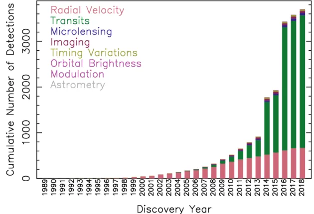
1.11 Cumulative exoplanet discoveries . . . 16
1.12 Properties of detected exoplanets . . . 17
1.13 Example of the radial velocity method . . . 18
1.14 Example of the directly imaged planet . . . 20
1.15 Example of planet detected with microlensing . . . 21
1.16 Illustration of the transit method . . . 23
1.17 Observed transit of WASP-25b . . . 24
1.18 TheKepler telescope . . . 25
1.19 Kepler rocky habitable zone planets . . . 26
1.20 Kepler resolution compared to Robo-AO . . . 27
1.26 Odd-even false positive test . . . 36
1.27 Centroid false positive test . . . 37
1.28 Secondary eclipse false positive test . . . 38
1.29 Ephemeris matching false positive test . . . 40
2.1 Simulated planets discovered by TESS . . . 45
2.2 Performance simulations of Robo-SOAR . . . 46
2.3 Robo-SOAR schematic of major components . . . 46
2.4 Robo-SOAR optomechanical design . . . 49
2.5 Rendering of dual knife-edge WFS . . . 50
2.6 Prototype dual knife-edge wavefront sensor . . . 52
2.7 Robo-SOAR testbed . . . 53
3.1 Cool Subdwarfs HR diagram . . . 56
3.2 Dwarf multiplicity as a function of stellar mass . . . 57
3.3 Reduced proper motion diagram of rNLTT . . . 59
3.4 Properties of observed cool subdwarfs . . . 60
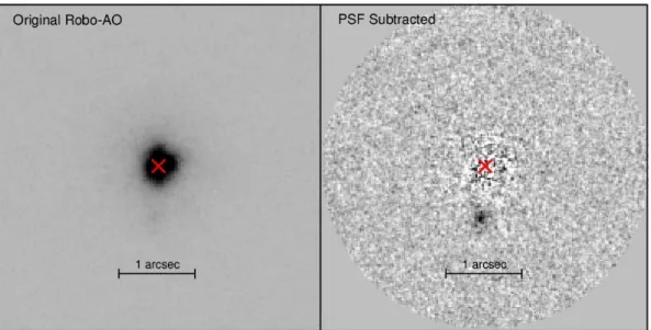
3.5 Example of PSF subtraction on cool subdwarfs . . . 64
3.6 Example of cool subdwarf spectra . . . 66
3.7 Keck-AO image of cool subdwarf confirming Robo-AO detection . . . 70
3.8 Comparison of companions to M-dwarfs and subdwarfs . . . 71
3.9 Properties of Keck confirmed subdwarf companions . . . 72
3.10 Cutouts of close subdwarf companions . . . 73
3.11 Binary fraction of cool subdwarfs as a function of color . . . 74
3.12 Comparison of companion contrasts between M-dwarfs and subdwarfs . . . 76
3.13 Comparison of separations of companions to M-dwarfs and subwarfs . . . 78
4.1 Properties of KOIs observed in the Robo-AO KOI survey . . . 83
4.2 On-sky positions of targeted KOIs . . . 86
4.4 Cutouts of observations of KOIs with Keck . . . 95
4.5 Cutouts of observations of KOIs with Gemini North . . . 97
4.6 Multiplicity fraction as a function of KOI number . . . 100
4.7 Nearby star fraction as a function of effective temperature . . . 101
4.8 Nearby star fraction of single and multiple planet systems . . . 103
4.9 Nearby star fraction of KOIs as a function of period and size . . . 104
4.10 Nearby star fraction of likely bound KOIs as a function of period and size . . . . 105
4.11 Multiplicity fraction of four planetary populations . . . 105
4.12 Likely bound multiplicity fraction of four planetary populations . . . 106
4.13 Multiplicity fraction as a function of orbital semi-major axis . . . 107
5.1 Properties of KOIs observed with Robo-AO . . . 109
5.2 LP600 passband . . . 111
5.3 Properties of detected nearby stars to KOIs . . . 112
5.4 KOI nearby star fraction as a function of separation . . . 115
5.5 Keck-AO imaging of KOI-3214 . . . 125
5.6 Archival images of KOI-3214 . . . 125
5.7 Keck-AO imaging of KOI-3463 . . . 127
5.8 Archival images of KOI-3463 . . . 127
5.9 Keck-AO imaging of KOI-4495 . . . 129
5.10 Archival images of KOI-4495 . . . 130
5.11 Keck-AO imaging of KOI-5327 . . . 131
5.12 Archival images of KOI-5327 . . . 131
6.4 Observed stellar densities in Kepler field . . . 142
6.5 Location on the sky of KOIs with nearby stars . . . 143
6.6 Nearby star fraction as a function of KOI number . . . 145
6.7 Nearby star fraction as a function of Teff . . . 146
6.8 Nearby star fraction as a function of Teff (CKS) . . . 146
6.9 Nearby star fraction of single and multi-planet systems . . . 148
6.10 Nearby star fraction as a function of planet size and period . . . 151
6.11 Nearby star fraction and stellar metallicity . . . 153
7.1 Simulated planets discovered by TESS . . . 157
7.2 Example of lucky imaging . . . 159
7.3 Publications by LGS-AO system . . . 160
C.1 Cutouts of KOIs with nearby stars observed with Keck-AO . . . 180
C.2 Cutouts of KOIs with nearby stars observed with Keck-AO . . . 181
F.1 Cutouts of KOIs with nearby stars observed with Robo-AO . . . 208
F.2 Cutouts of KOIs with nearby stars observed with Robo-AO . . . 209
F.3 Cutouts of KOIs with nearby stars observed with Robo-AO . . . 210
F.4 Cutouts of KOIs with nearby stars observed with Robo-AO . . . 211
F.5 Cutouts of KOIs with nearby stars observed with Robo-AO . . . 212
F.6 Cutouts of KOIs with nearby stars observed with Robo-AO . . . 213
F.7 Cutouts of KOIs with nearby stars observed with Robo-AO . . . 214
F.8 Cutouts of KOIs with nearby stars observed with Robo-AO . . . 215
F.9 Cutouts of KOIs with nearby stars observed with Robo-AO . . . 216
LIST OF TABLES
3.1 The specifications of the Robo-AO subdwarf survey . . . 62
3.2 Full SOAR Spectroscopic Observation List . . . 67
3.3 Keck-AO Cool Subdwarf Observations . . . 69
4.1 The specifications of the Robo-AO KOI survey . . . 85
4.2 Full Keck-AO Observation List . . . 94
4.3 Full Gemini Observation List . . . 95
5.1 The specifications of the Robo-AO KOI survey . . . 110
5.2 Robo-AO KOI Survey Cumulative Nearby Star Fraction Rates . . . 114
5.3 Nearby Star Fraction Rates By Planet Candidate Type . . . 114
5.4 Planetary Candidates Likely Not Rocky Due to Nearby Stars . . . 117
5.5 High-order multiple KOIs resolved using Keck-AO . . . 122
5.6 Photometric distance estimates of high-order multiple KOIs . . . 123
5.7 Corrected radii of planetary candidates in potential high-order multiple systems 124 A.1 Multiple subdwarf systems resolved using Robo-AO . . . 162
B.1 Measured properties of detected nearby stars to KOIs . . . 164
C.1 Keck-AO KOI Observation List and Detected Companions . . . 178
D.1 Updated Kepler Planetary Candidate Radii . . . 182
LIST OF ABBREVIATIONS AND SYMBOLS
AO Adaptive Optics
CCD Charge-coupled Device CKS CaliforniaKepler Survey
DM Deformable Mirror
DSS Digital Sky Survey FWHM Full Width Half Max KOI Kepler Input Catalog KOI Kepler Object of Interest
LGS-AO Laser Guidestar Adaptive Optics log g log of the surface gravity (cm s−2) NGS-AO Natural Guidestar Adaptive Optics NIR Near Infrared
NLTT New Luyten Two-Tenths catalog OAP Off-Axis Parabolic mirror
PM Proper Motion
PRF Pixel Response Function PSF Point Spread Function PWFS Pyramid Wavefront Sensor RPM Reduced Proper Motion SDSS Sloan Digital Sky Survey SED Spectral Energy Distribution
Teff Effective Temperature
CHAPTER 1: INTRODUCTION
Space, it says, is big. Really big. You just wont believe how vastly,
hugely, mindbogglingly big it is. I mean, you may think its a long
way down the road to the chemists, but thats just peanuts to space.
— The Hitchhiker’s Guide to the Galaxy
In the last decade, astronomy has entered an era of large surveys and big data. The emergence of inexpensive detectors and robotic telescopes have contributed to the advent of wide-field surveys in both space and on the ground that deliver a plethora of discoveries. Some of these surveys, such as the Evryscope (Law et al., 2015), observe tens of millions of stars continuously throughout a night. They are able to detect a single star brighten or dim over the span of a few minutes. Others, such as Kepler, are adept at observing fewer stars but with high photometric precision, searching for a periodic signal consistent with an exoplanet.
This thesis presents the use of robotic adaptive optics to study exoplanets and stellar populations. The unparalleled efficiency provided by automated instruments are proving themselves vital in the current era of astronomy. I used the robotic instrument, Robo-AO, to provide the high-resolution images needed to understand the properties of thousands of planetary candidates. I also present a study into the multiplicity of cool subdwarfs, remnants of the first stars formed in the galaxy. I also present the design and construction of a new robotic instrument, Robo-SOAR, an NGS-AO system to be mounted on the SOAR telescope. In this introduction, I first describe the design of adaptive optics and the Robo-AO system. I conclude with an overview of the state of the exoplanet field, theKepler spacecraft, and the role of ground-based follow-up observations.
1.1 Automated Adaptive Optics
1.1.1 Adaptive Optics
Atmospheric Seeing
Adaptive optics (AO) is a method to remove wavefront aberrations in light from astro-physical sources caused by turbulent inhomogeneities in the Earth’s atmosphere, as illus-trated in Figure 1.1. These turbulent layers have different temperatures and wind velocities, leading to slightly different indices of refraction. An incoming plane wave will be distorted as it moves through these different regions in the atmosphere. The turbulence in the atmo-sphere is usually characterized by a measure of the atmospheric correlation length, the Fried parameter (Fried, 1967), or r0.
Figure 1.1: In this illustration, light from an astrophysical object consisting of initially plane wavefronts is perturbed when entering the atmosphere by turbulent layers, resulting in corrugated wavefronts at the ground. [Image courtesy of D. Buscher]
seeing disk scales withλ−1/5, i.e. seeing improves at longer wavelengths.
At excellent observing sites, seeing is typically on the order of an arcsecond. Conse-quently, while large telescopes have theoretically sub-arcsecond resolution limited only by diffraction, they will in practice have a resolution equal to the atmospheric seeing. A survey of exoplanet candidate hosts with seeing-limited resolution would not detect the majority of previously unknown nearby stars contaminating the photometry.
Basic Design
Figure 1.2: From the left, simulated images of a point source of light seen through a diffraction-limited telescope of diameter d, a short exposure of the point source through the same telescope and with atmospheric seeing with a Fried parameter given by r0 = 0.1d, and seen in a long exposure with the same telescope and seeing, revealing the seeing disc.
tip-tilt mirror, a mirror which can move in two directions, is positioned earlier in the optical path and used to correct low-order wavefront errors. After reflecting off the DM, the light is refocused with a second OAP. The light is split using a beamsplitter either before or after this second OAP. Some of the light is sent to the science detector and used to image the target. The rest of the light, typically wavelengths not required for the science, is sent to a wavefront sensor.
Wavefront Sensing
A wavefront sensor (WFS) is used to measure the aberrations in the wavefront. With this information, the position of the tip-tilt mirror and the DM shape can be set such that the resulting wavefront is nearly flat. In “open loop” operation, the WFS measures the wavefront before any correction has been applied. In “closed loop” operation, the wavefront error is measured by the WFS after correction by the tip-tilt mirror and DM, and the residual errors will be small.
A WFS requires a bright source, a guidestar, that can be used to measure the wave-front distortions. As the science target is often too faint to be used as a guidestar, a bright (V<12) nearby star may be used, called natural guidestar AO (NGS-AO). Often, however, a sufficiently bright star will not be found nearby, resulting in NGS-AO systems having limited sky coverage (Ellerbroek & Andersen, 2008). Alternatively, an artificial guidestar created with lasers may be used, called laser guidestar AO (LGS-AO). These systems typically em-ploy either a Rayleigh laser, which uses high-altitude backscattering from a near ultraviolet laser or a sodium laser, which uses a 589nm laser to excite a layer of sodium atoms in the upper atmosphere that originate from meteor ablation. A faint natural guidestar is typically still required for image position information, although high-order-only wavefront corrections result in significant image quality gains compared to seeing-limited imaging (Howard et al., 2018). These systems have nearly unlimited sky coverage, but the added complexity increases observing overhead time.
Figure 1.4: A schematic of a Shack-Hartmann WFS. The distorted wavefront is incident on the lenslet array. The position of the imaged source is displaced slightly from the nominal position due to aberrations in the wavefront. [Figure courtesy of Wikipedia Commons]
then be reconstructed from the displacement of these images. Shack-Hartmann WFS are relatively inexpensive and simple devices. They require a relatively bright reference star as the pupil is re-imaged into, in some systems, hundreds of sub-pupils, each required to be sufficiently bright to measure the incoming wavefront slope. When used in NGS-AO system, this requirement greatly limits the sky coverage possible with AO correction.
the wavefront is distorted, the slope of the incoming waveform will alter which quadrant of the pyramid it passes through, and the pupils will be differentially illuminated. To improve linearity (i.e. be able to detect very small wavefront aberrations), the focused beam is often modulated in a circular pattern around the pyramid apex (Fauvarque et al., 2015). The slope of the incoming wavefront at any sub-aperture can be calculated from the intensity in four corresponding pixels in each pupil image. If these intensities are given by S1, S2, S3, and S4 (corresponding to the pupils imaged in Figure 1.5), the slopes of the wavefront, W, in that sub-aperture in the x- and y-direction are given by the relations
δW
δx =δθx
(S1+S3)−(S2+S4)
S1+S2+S3+S4
(1.1.1)
δW δy =δθy
(S1+S2)−(S3+S4)
S1+S2 +S3+S4
(1.1.2)
where θx and θy is the amplitude of modulation in the x- and y-directions.
The PWFS allows considerable optimization for observations with low-brightness refer-ence stars. Since the sub-apertures are set by the pixels on the detector, dynamic binning of these pixels can perform lower-order wavefront corrections even with faint reference stars. In addition, the frequency and amplitude of modulation may be adjusted to increase the performance of the system. This greatly increases the sky coverage where some level of AO corrections may be applied.
Figure 1.6: On the right, the input pyramid for the Large Binocular Telescope with diameter 13mm. On the left, the aluminum “mother pyramid” used in manufacturing, with the glass pyramid at its vertex. [Image courtesy of A. Tozzi]
significant chromatic aberrations arise in the pupil image. This is caused by the wavelength dependence of the refractive index of the glass. The pupil drift at the blue and red extremes can be as much as several CCD pixels. To reduce these aberrations, achromatic double pyramids are typically used (Tozzi et al., 2008), further increasing the potential cost.
In Chapter 2, I describe the design and construction of a reflective pyramid WFS design, costing substantially less than glass optics with reduced chromatic aberrations in the output pupil images.
1.1.2 Robo-AO
Figure 1.7: The acquisition times for the LGS-AO system on Keck. The acquisition time includes all telescope and AO overheads, including slews. The average overhead for this conventional AO system of 9 minutes is substantially longer than the 40 seconds of Robo-AO. [Image courtesy of David Le Mignant]
years with new surveys coming online, such as TESS (Ricker et al., 2014) and LSST (Tyson, 2002).
Figure 1.8: Robo-AO mounted on the automated 1.5-m telescope at Palomar Observatory. [Image courtesy of Christoph Baranec]
Robo-AO Instrumentation
Robo-AO Observations
The observing sequence for a single target, described in detail in Baranec et al. (2014a), begins with a queue scheduling program that optimizes among scientific priority, slew time, telescope limits, prior observing attempts, and laser-satellite avoidance windows. The science camera, laser, and adaptive optics system are configured as the telescope slews, typically taking 40 seconds. Once pointed at the new target, the laser is acquired with a search algorithm moving a steering mirror. This process takes approximately 40 seconds, during which time the adaptive optics system is started and an observation is performed with no adaptive optics correction to estimate seeing conditions. Once the laser is acquired, the adaptive optics correction is started, removing residual atmospheric wavefront aberrations at 100Hz using a 12×12 actuator deformable mirror. The science field is imaged at 8.6Hz and saved in data cubes for later processing.
At Palomar, Robo-AO performed over 19,000 observations (see Figure 1.10), including the majority of the KOI observations, detailed in Chapter 4. In 2015, Robo-AO relocated to the Kitt Peak 2.1-m telescope for a 3-year deployment (Jensen-Clem et al., 2017). A near-infrared avalanche photodiode array camera was added to the system, enabling simultaneous visible and infrared imaging.
We describe in Chapter 2 the design and construction of Robo-SOAR, an NGS-AO analog to Robo-AO, that will observe in the South and bring automated high-resolution imaging to the entire sky.
1.2 Exoplanet Confirmation and Characterization
Figure 1.9: The optical design of Robo-AO. (Baranec et al., 2014a)
Sun. In only the last few decades, we have discovered thousands of other planetary systems1 around other stars. A planet has even been detected around the nearest star (Anglada-Escud´e et al., 2016). Planets, it seems, are common in the galaxy and planetary systems similar to our own are not unusual.
The most probable scenario, as far as is known, for life to exist in the galaxy is on rocky exoplanets or exomoons, warmed sufficiently by starlight or internal processes for liquid water, or alternative solvent (Schulze-Makuch et al., 2011), to subsist (Lammer et al., 2009). Studying exoplanets provides insight into the prevalence of Earth-like planets, and concurrently life, in the galaxy. Current observational resources are capable of detecting these planets and measuring the planetary radii and mass, leading to estimates of the planetary bulk densities and compositions. Future telescopes, such as the new generation of extremely large telescopes and the James Webb Space Telescope (Greene et al., 2016), will be capable in the next decade of detecting biosignatures in these planet’s atmosphere, strong indicators for the presence of life. These observations will be time-intensive and limited, and a primary objective of current surveys is to detect and thoroughly vet excellent targets suitable for further study.
Figure 1.11: The cumulative detections of exoplanets by year and by detection technique. The radial velocity method discovered the majority of exoplanets until the discoveries by the Kepler telescope using the transit method were confirmed, beginning in earnest in 2013. [Image courtesy of NASA Exoplanet Archive]
note particular strengths and limitations of each.
1.2.1 Detection Techniques
Pulsar Timing Variations
The first exoplanets were detected in 1992 around a millisecond pulsar (Wolszczan & Frail, 1992). Pulsars are rapidly spinning, compact stellar remnants that emit beams of electromagnetic radiation (Pacini, 1967). The frequency of these beams as observed from Earth is very regular, even rivaling atomic clocks (Matsakis et al., 1997). The influence of planets orbiting the pulsar will introduce slight anomalies into the pulsar timing which may be used to reveal the parameters of the planetary orbit and the planetary mass.
Figure 1.13: Example of a radial velocity detection of a≥3.6 Earth-mass exoplanet orbiting just inside the habitable zone of the nearby K-type star, HD 85512. The velocity measure-ments are folded to the 58.4 day period of the planet. [Image from Pepe et al. (2011)]
0.1 Earth masses, as well as planets at long period orbits. Pulsars with orbiting planets are rare, however, and only four pulsar planetary systems have been detected to date. In recent years, variations in the timing of stellar pulsations of hot subdwarf and main-sequence stars have been used to detect several planetary candidates (Silvotti et al., 2007; Murphy et al., 2016).
Radial Velocity
The gravitational influence of an orbiting planet will induce velocity variations in the host star, typically on the order of a few meters per second. The light from the star is Doppler shifted due to these velocity variations. High-resolution spectroscopy is able to measure the line-of-sight stellar velocity using the slight shift of emission and absorption lines in the stellar spectra. With velocity measurements from observations over multiple epochs, the influence of an unseen planet on the host star can be revealed, as shown in Figure 1.13.
of orbital inclinations. Because the star-planet interaction is mediated by gravity, smaller planets result in lower stellar velocity amplitudes and are thus difficult to detect. In addition, the measurements required to detect and study a single planet are time-intensive and require a large-aperture telescope and stable, high-resolution spectrographs.
In 1995, the first exoplanet was discovered around a main-sequence star, 51 Pegasi b, using the radial velocity technique (Mayor & Queloz, 1995). This method dominated the exoplanet discovery field for over a decade and revealed many surprises, such as the existence of “hot Jupiters.” Since 2011, the number of detected exoplanets with radial velocity has declined, as telescope time has been dedicated to follow-up planets from transit surveys. New instruments in the coming years, such as NEID (Halverson et al., 2016), will be sensitive to velocity amplitudes as low as 10 cm−1, consistent with an Earth-size planet orbiting at 1 AU.
Direct Imaging
The majority of exoplanets have been discovered by indirect measurements, observing their effect on more visible objects. Imaging a spatially resolved planet is an enormous challenge, as the host star emits far more light than the planet. For illustration, if a twin of our solar system were placed at 10 parsecs, Jupiter, the brightest planet, would emit only around 10−9 the flux of the parent star at an angular separation of 0.5”.
Figure 1.14: Directly imaged planets orbiting HR8799, observed in the near-infrared with Keck adaptive optics. The four planets range from 3 to 7 Jupiter masses. The light from the central star has been reduced in intensity with a coronograph. [Image from Marois et al. (2010)]
planets 10−5 fainter than the host star at separations of 1”. An example of directly imaged planets is shown in Figure 1.14.
The first image of an exoplanet, the five Jupiter-mass 2M1207b which orbits a brown dwarf, came in 2004 (Chauvin et al., 2004). A total of 18 more planetary systems have been imaged in the intervening years, far fewer than was initially expected2. This suggests a significant discrepancy exists between the planet mass function extrapolated from radial velocity surveys and the true giant exoplanet mass function (Bowler, 2016).
Future instruments on extremely large telescopes and the proposed coronagraphic capa-bility for the 2.4m space-based WFIRST mission (Spergel et al., 2013) will allow imaging
2Macintosh et al. (2006) suggested that nearly 100 planets could be discovered with GPI. In the first 2.5
Figure 1.15: A Neptune-sized planet detected with the microlensing method. The brightness of the background star is observed. Gravity from the planet, orbiting the foreground star, contributes to the magnification of the background star. [Image from Sumi et al. (2010)]
of planets at close orbits and be sensitive to reflected starlight. At their theoretical per-formance limit, these instruments could even detect rocky planets in the habitable zone of nearby M-dwarfs (Guyon et al., 2012).
Microlensing
and Microlensing Observations in Astrophysics (MOA, Bond et al., 2004) surveys.
Microlensing is able to detect planets at wide-orbits, low-mass planets (down to Mars-size with WFIRST), and planets around distant stars. The planetary mass can be loosely constrained from microlensing, as well as the planet’s separation from the host star at the time of the lensing event. A microlensing event only happens a single time, however, and the host star is often too distant for follow-up observations, severely limiting characterization of any detected planetary system.
Astrometry
The astrometric method for detecting planets uses precise measurements of a star’s position in the sky. Both components in a planet-star system orbit their mutual center of mass or barycenter. The astrometric method seeks to observe the small shift in stellar position as a star orbits the system barycenter. The variation in position is so small that ground-based telescopes, contending with the effects of atmospheric turbulence, have not yet been able to detect any planets with this method. The Hubble Space Telescope did use astrometry to determine the mass of a previously known planet, Gliese 876b (Benedict et al., 2002).
The Gaia space telescope will provide microarcsecond astrometric precision for the brightest stars, and is expected to discover approximately 20,000 long-period planets with masses between 1-15 Jupiter masses within 500 pc (Perryman et al., 2014). If extended for a 10-yr mission, the number of planet detections will more than triple.
1.2.2 Transit Method
Figure 1.16: An illustration of the transit method, which detects exoplanets by looking for the small decrease in brightness of the host star as the planet orbits in front of its disk. [Image courtesy of TESS Science Team]
fundamental properties of the exoplanet. The time between successive transits provides the period of the planet. The radius of the exoplanet can be estimated from the depth of the transit or change in observed stellar flux, ∆F, using the equation
∆F
F =
R2p R2
?
(1.2.1)
where Rp is the radius of the planet and R? is the radius of the occulted star.
Figure 1.17: The transit of hot Jupiter, WASP-25b, as observed with the Goodman spectro-graph (Clemens et al., 2004) on SOAR. The black solid line is a transit model fit with the Python package batman (Kreidberg, 2015). The lower dashed line shows residuals from the transit model.
decade. These discoveries were mostly gas giants orbiting at low periods, in part due to the low photometric precision (Fhring et al., 2015) achieved with small telescopes on the ground (sensitivities to flux variations of a few thousand parts per million is typical for these surveys). The inherent occurrence rate in the galaxy of Earth-like planets, i.e. rocky planets orbiting within the habitable-zone of their host star, was difficult to estimate from ground-based surveys alone. To find small planets that could maintain liquid water, exquisite photometry of thousands of stars over a multi-year baseline is required. This is only feasible with a space-based telescope.
The European Space Agency CoRoT mission (Barge et al., 2008) launched in 2006, with a primary mission of detecting terrestrial planets at low-period orbits. However, CoRoT-7b (L´eger et al., 2009), with an estimated radius of 1.7R⊕, was the only potentially rocky planet
Figure 1.18: (a) A sketch of theKepler telescope mated to the spacecraft. (b) The assembled flight system in a clean room with the telescope dust cover in place. The dust cover was ejected after launch. Note the person at the lower left for scale. (Courtesy of BATC)
1.2.3 Kepler Telescope
Figure 1.19: Properties of the potentially habitable exoplanet candidates discovered by Ke-pler. The effective stellar temperature of the host star is plotted on the y-axis, and the incident stellar flux at the orbit of the planet in units of Earth-flux is plotted on the x-axis. Planets with derived radii less than 2.5R⊕ are labeled, and solar system planets are plotted
Figure 1.20: On the left, a high-resolution image from Robo-AO of KOI-4418 (KIC2859893) rotated and scaled to match the Kepler view of the same field, displayed on the right, with each pixel colored by the mean flux in Quarter 4. KICs in the field are marked in both images. The 1.41” binary to KOI-4418 is not visible in the ∼4” pixels of Kepler, illustrating how real companions and background stars can blend with the KOIs, resulting in astrophysical false positives or inaccurate planetary property estimates. High-resolution follow-ups are a crucial step in the validation and characterization of Kepler planetary systems.
1.2.4 Photometric Contamination
Figure 1.21: Several scenarios exist for each KOI followed up: a) no nearby star is detected, and the statistical argument that a bona fide planet orbits in the system is strengthened; b) a nearby star is detected, then the contaminating flux from that star can be measured and the planetary radius estimate can be corrected; c) a nearby star is detected, which is the source of a false positive planetary transit signal, such as a background eclipsing binary.
1.2.5 The Need For High-resolution Follow-up Observations
Many of these false positive scenarios can be ruled out if no nearby star to the KOI is observed. The majority ofKepler targets are solar-type (Batalha et al., 2013), and most form with at least one companion star (Duquennoy & Mayor, 1991; Raghavan et al., 2010). These stars are often at separations from the KOI that cannot be resolved withKepler, as illustrated in Figure 1.20. Most stars within approximately 3” of the KOI are also not resolved in seeing limited surveys from the ground, such as DSS or UKIDSS images. All planetary candidates discovered with light curves produced byKepler must, therefore, be independently validated by ground-based high-angular resolution observations. As illustrated in Figure 1.21, these observations help confirm and characterize these planetary candidates in several ways.
No nearby star detected
to the explanation of a planet transiting the presumed target star. Accurate knowledge of the target star is required for this technique, usually derived from high-resolution imaging as well as from spectroscopy and astroseismology. A single stellar source within the photometric aperture significantly increases the probability that abona fideplanet is present in the system (Morton et al., 2016).
Real planet in system with nearby star
If a nearby star is detected, the contaminating flux from that star can be measured and the planetary radius may be re-derived. If a target star is blended with another star (bound or line-of-sight), the true planet radius is larger than the derived planet radius because the observed transit depth is diluted by the companion star (see Figure 1.22).
In general, we do not know which star the planet is orbiting. If the planet orbits the primary star, we can correct for the transit dilution with the equation,
Rp,A =Rp,0
r
1
FA
(1.2.2)
where Rp,A is the corrected radius of the planet orbiting the primary star, Rp,0 is the original planetary radius estimate based on the diluted transit signal, and FA is the fraction of flux
within the aperture from the primary star.
For the case where the planet candidate is bound to the secondary star, we use the relation
Rp,B =Rp,0
RB RA
r
1
FB (1.2.3)
where Rp,B is the corrected radius of the planet orbiting the secondary star bound to the
Time
B
ri
gh
tn
es
s
Depth
Planet transiting
single star
Nearby star
contamination
Flux
host
-1
Figure 1.22: An illustration of the impact contaminating flux from a nearby star has on the transit depth of a planet. On the left, a planet transiting a single star. The radius of the planet can be derived from the depth of the transit. On the right, a planet transiting a star with a flux contribution from a nearby star. The additional flux will result in a shallower transit depth with respect to the single star system. The radius of the planet can be estimated with an additional term containing Fluxhost, the fraction of the flux in the
the radius correction factor can vastly increase. The impact on the derived planetary radius of the two scenarios is illustrated in Figure 1.23.
These radius corrections can have an enormous impact on our understanding of the planetary candidate properties. With tight constraints on the planetary radius provided by transit observations coupled with mass measurements from either radial velocity observa-tions or transit timing variaobserva-tions (Mazeh et al., 2013), the planetary bulk density may be estimated. Fitting the bulk densities to models allows the composition of the exoplanet to be inferred (Spiegel et al., 2014), as shown in Figure 1.24.
If all stars are assumed to be single, as is the case for every KOI initially, the planetary radii will be underestimated, on average, by a factor of 1.5 (Ciardi et al., 2015). The density of the planet scales with the cube of the planetary radius. Therefore an increase in the radius estimate by 1.5, typical of KOIs with detected nearby stars, will decrease the bulk density by a factor of approximately 3.4. In summary, the occurrence rate of Earth-size planets will be overestimated by as much as 15-20% if all stars are assumed single.
It is believed that the transition between rocky planets and those with a large gaseous envelope occurs rather sharply at around 1.5 to 1.6R⊕ (Rogers, 2015; Weiss & Marcy, 2014).
For example, KOI-2598.01 is a planet candidate with an original derived radius of 1.35R⊕,
using the Kepler light curve alone (Batalha et al., 2013). A host star was resolved in imaging using a high-angular resolution instrument into a near-equal brightness binary with a separation of approximately 1” (Baranec et al., 2016). The additional contaminating flux from this previously unknown star, blended with the primary in theKepler image, diluted the transit, making it appear shallower than it would from a single star system. Since the radius estimate of the planetary candidate is directly related to the depth of the transit, as shown in Equation 1.2.1, the corrected derived radius will always be larger when a nearby star is discovered. In this case, if the planet orbits the primary star, the corrected planetary radius is 1.77R⊕. If instead, the planet orbits the secondary star which is bound to the primary
radius is 2.0R⊕. In either case, the estimated planetary radius is no longer consistent with
a rocky planet with a thin atmosphere.
No planet in system with nearby star
As illustrated in Figure 1.25, there are several alternative scenarios which mimic a real planet orbiting the primary star:
a) a brown dwarf star orbiting the primary star. Brown dwarfs are deuterium burning stars that have approximately the same radius as Jupiter (Chabrier et al., 2009), but can have masses up to 80 MJ. The transit depth of these systems is therefore similar to a gas
giant planetary system, but radial velocity observations must be used to break the mass-radius degeneracy (Santerne et al., 2013). The majority of KOIs, however, are too faint (V>14) for precision radial velocity (Fressin et al., 2013).
b) a background eclipsing binary, blended with the primary star. Their faintness with respect to the nearby KOI can reduce their deep transit depths, on the order of tens of percent when observed alone, to a depth of a few percent, consistent with the transit of a large planet (Abdul-Masih et al., 2016).
c) a grazing stellar binary. The full disks of the binary stars do not overlap each other, resulting in a distinctive V-shaped transit (Koch et al., 2007).
The false positive rate of KOIs is significantly lower than that of candidate planets from ground-based transit surveys (for example,∼80% for HAT-Net (Latham et al., 2009)). This is the result of the extensive vetting performed by the Kepler science team (Batalha et al., 2013). Before being elevated to planet candidate status, each threshold crossing event (instances when the transit detection significance for a star with a given planetary orbital period and epoch exceeds 7.1σ, over 34,000 in total over theKepler mission) is checked for clear signatures of being an astrophysical false positive. A few of the tests that all KOIs must pass are:
Figure 1.26: An example of the odd-even transit test used to detect near equal mass eclipsing binaries from the Kepler DR25 vetting reports. Points from the odd- and even-transits are shown in red and blue, respectively. A best-fit transit model is shown by the solid black line. In this example, the odd- and even-transits both fit the transit model. [Image courtesy of Jeff Coughlin]
transits (the second, fourth, sixth, etc.) can determine if the transit signal is an eclips-ing binary with two nearly equal mass and size stars. In these cases, we expect slight variations in the transit depth between the two sets of transits, as the star being eclipsed alternates. An example of this test is given in Figure 1.26.
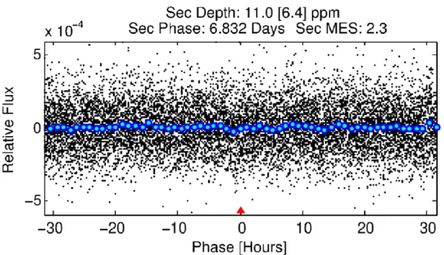
Figure 1.28: An example of the secondary eclipse test from theKepler DR25 vetting reports. If the eclipsing body is self-luminous, we would expect a significant secondary eclipse in the light curve. The strongest secondary eclipse candidate of a transit event is displayed with raw Kepler data in black and the phase-binned averages of the data in blue. The depth of this secondary eclipse, indicated with a red triangle, is approximately 11 parts per million, and this candidate is not considered a significant secondary eclipse. [Image courtesy of Jeff Coughlin]
secondary eclipse as the eclipsing object is self-luminous. The secondary eclipse will likely be significantly shallower than the primary transit and will occur a half-phase after the primary transit if the eccentricity of the system is near zero. It is possible for hot Jupiters to have secondary eclipses due to reflected starlight, with detectable depths in the visible passband in whichKepler observes. To pass the test, the properties of a detected eclipse must be consistent with that expected for a planet with the estimated radius and orbital period (Angerhausen et al., 2015). An example of the secondary eclipse test is shown in Figure 1.28.
If the transit signal has similar ephemerides, that is the same period and epoch, to that of a known transient source, such as an eclipsing binary, the transit is likely a false positive due to contamination. These false positive transit signals can be caused by stellar crowding, diffraction spikes, ghosting, or electronic cross-talk. An example of ephemeris matching performed on KOIs is shown in Figure 1.29.
While these vetting efforts on early catalogs were largely based on human inspection (Batalha et al., 2010), the most recent DR25 catalog has fully automated this process (Cough-lin et al., 2016).
After this initial vetting, a relatively large number of false positive KOIs remain. This is in part due to a preponderance of caution by the Kepler team to not remove real planets from the candidate list. Notably, the candidate status of a KOI isnot a function of its depth or shape (i.e., whether it is V-shaped, which has a high probability of being caused by an eclipsing binary but can conceivably be produced by grazing transiting planets, as well). This means that a large fraction of the deeper signals (∼50%) can be expected to be false positives (Santerne et al., 2012, 2015). Shallower candidates have a much lower predicted false positive rate (∼10%) (Morton & Johnson, 2011; Fressin et al., 2013), a prediction that has been confirmed by follow-up observations from theSpitzer space telescope (D´esert et al., 2015). Lastly, it has been determined that almost all multiple-planet candidate systems are in fact real, physically associated planetary systems (Lissauer et al., 2012).
survey that does just that in Chapters 4, 5, and 6.
1.3 Overview of Contents
This dissertation is divided into three sections: confirmation and characterization of exoplanets with robotic adaptive optics, multiplicity study of cool subdwarfs, and the design and construction of Robo-SOAR, a Southern robotic NGS-AO system.
In Chapter 2, I present the design and construction of Robo-SOAR. An NGS-AO analog to Robo-AO, Robo-SOAR will be a high-order AO system providing robotic AO observing to the South. The design includes a novel WFS design, a reflective version of a PWFS, which is significantly less costly than traditional glass pyramids.
In Chapter 3, I present the Robo-AO observations of 350 cool subdwarfs, an order of magnitude more targets than every other high-resolution cool subdwarf survey combined. I find these stars have significantly lower binarity rates than similar dwarf stars. I discuss how metallicity can impact binarity rates and what the results tell us about the early galaxy.
In Chapter 4, I introduce the Robo-AO KOI survey, beginning with high-resolution ob-servations of 1629 planetary candidates. I use these obob-servations to study the impact that stellar binarity has on planetary systems. In Chapter 5, I describe the cumulative statis-tics from the full survey consisting of observations of approximately 4000 Kepler planetary candidate hosts. I provide corrected radii estimates for over 800 planetary candidates. In Chapter 6, I continue the analysis of the results of the KOI survey, with characterization of the discovered nearby stars. I then apply more sophisticated analysis to understand how planetary systems are affected by binary stars.
• Fulton, B. J., Collins, K. A., Gaudi, B. S., et al. 2015, ApJ, 810, 30 – Reduced and analyzed Robo-AO observations of the host star of KELT-8b, a highly inflated hot Jupiter.
• David, T. J., Stauffer, J., Hillenbrand, L. A., et al. 2015, ApJ, 814, 62 – Reduced and analyzed Robo-AO observations of HII 2407, an eclipsing binary in the Pleiades. • Schlieder, J. E., Crossfield, I. J. M., Petigura, E. A., et al. 2016, ApJ, 818, 87 – Reduced
and analyzed Robo-AO observations of the host star of K2-26, a small terrestrial planet orbiting an M-dwarf.
• Atkinson, D., Baranec, C., Ziegler, C., et al. 2017, AJ, 153, 25 – Reduced multi-band Keck-AO images used to access the probability of association of nearby stars to 104 KOIs.
• Crossfield, I. J. M., Ciardi, D. R., Petigura, E. A., et al. 2016, ApJS, 226, 7 – Reduced and analyzed Robo-AO observations of 197 planetary candidates from K2, contributing to the confirmation of 104 planets.
• Adams, E. R., Jackson, B., Endl, M., et al. 2017, AJ, 153, 82 – Reduced and analyzed Keck-AO observations of EPIC 220674823, host star to an ultra-short period planet (0.57d) and one additional planet.
• Schonhut-Stasik, J. S., Baranec, C., Huber, D., et al. 2017, ApJ, 847, 97 – Assisted in the reduction and analysis of Robo-AO and Keck-AO images of 99 astroseismic gold standard stars observed with Kepler.
CHAPTER 2: ROBO-SOAR: SOUTHERN ROBOTIC NGS-AO
A common mistake that people make when trying to design
something completely foolproof is to underestimate the ingenuity of
complete fools.
— The Hitchhiker’s Guide to the Galaxy
In this chapter, I discuss the design and construction of Robo-SOAR. This chapter contains content originally from Ziegler et al. (2016).
The automation of adaptive optics observing, allowing unprecedented time-efficient ob-servations, has been proven successful and worthwhile by the Robo-AO system (Riddle et al., 2012; Baranec et al., 2013, 2014a). Expanding this capability to the larger SOAR telescope and providing access to the Southern-Hemisphere is the purview of the Robo-SOAR in-strument. Coupled with the already operational Northern Robo-AO system (Jensen-Clem et al., 2017), and planned further Northern Hemisphere systems in Hawaii and elsewhere, all-sky robotic observations of up to 1000 targets a night will be possible. This capability will be critical to follow-up planetary candidates discovered by TESS (Ricker et al., 2014), illustrated in Figure 2.1
2.1 System Capabilities
Figure 2.1: On-sky locations of simulated TESS planetary discoveries. Red dots are planets detected around the targeted stars, and blue dots are planets detected around stars in the full frame images. Robo-SOAR, in combination with Robo-AO, will be able to observe every TESS planet candidate host star in high-resolution. [Image courtesy of Sullivan et al. (2015)]
on Robo-AO, allowing observations of at least 10×more targets per hours than the similar MagAO system.
Using AO-assisted speckle-imaging, Robo-SOAR will achieve diffraction-limited visible-light performance on guide stars at least as faint as V=16, 1-2 magnitudes fainter than non-AO-assisted speckle imaging systems. Compared to lucky imaging systems, Robo-SOAR will attain an increase in angular resolution of at least a factor of 2 and ten times more light-collection efficiency. With an optional NIR camera upgrade path, detection of companions with 2-3× lower masses than other large-survey instruments is possible, including Robo-AO, as shown in Figure 2.2. Law et al. (2016) covers the science plans and capabilities of Robo-SOAR in more detail.
Figure 2.2: Detectable companions around typical stars in Robo-SOAR multiplicity surveys. The NIR camera is more effective at finding low-mass companions, and the visible camera will provide colors for mass estimates, improved angular resolution, and a passband that matches most large sky surveys. [Image from Law et al. (2016)]
larger seeing-limited field of view to enable automated target identification and alignment. An OAP relay will provide magnification of 2.26×, achieving Nyquist sampling for 30 mas visible-light diffraction-limited cores on the detector. An atmospheric dispersion corrector similar to Robo-AO’s design is placed in the collimated beam after the DM and before the second OAP. Visible light science images, with field-of-view approximately 17” square, are acquired by a photon-counting Andor iXon 888 EMCCD. An optional upgrade path has NIR light sent by a dichroic into a re-imaging relay and to a Princeton Instruments 640LN NIR InGaAs-array camera. The 640LN camera is liquid-nitrogen cooled, with significantly lower read noise and dark current (15e- and <8e-/pix/sec, respectively) than traditional off-the-shelf InGaAs cameras, allowing sky background limited observations in H-band. Tip/tilt correction will be provided by SOAR’s M3 rapid-actuation mirror. The telescope simulator consists of a single-mode-fiber-fed collimated beam focused to the correct F# with rotating plastic disks to simulate turbulence. Using a dichroic, part of the light will be sent from the science path to the WFS assembly. The wavelengths extracted will be dynamically switched using an interchangeable dichroic assembly depending on the science goals.
A schematic of the system is shown in Figure 2.3. The mechanical design is shown in Figure 2.4. The full Robo-SOAR Zemax model predicts, with perfectly-built and aligned optics and no atmosphere, center-of-field Strehl ratios at 656nm of 0.99, decreasing to 0.97 at the edge of the 17” field (Figure 2.4).
2.2.1 Software Design
The SOAR control software need only cover a smaller set of capabilities, as Robo-SOAR is initially planned to operate as a natural-guide-star system. The control software will be responsible for real-time wavefront reconstruction, DM control, tip/tilt removal, and queue-based scheduling. Modifications of the Robo-AO code for use in Robo-SOAR include: 1) upgrades of the system performance for the 492-actuator system; 2) alteration of the system for natural guide star operation, a new reconstructor for the dual knife-edge WFS, interface with the Andor cameras and 640LN NIR camera, interface to SOAR TCS, and automatic acquisition of guide star with the context camera along with fast tip/tilt spiral slews coupled with fast frame rate science WFS EMCCDs. The Robo-AO reduction pipeline (Law et al., 2014; Ziegler et al., 2015, 2017a) will automatically calibrate and co-add the EMCCD visible-light camera data and then perform automated PSF subtraction and companion detection.
2.3 Dual Knife-edge WFS
The Robo-SOAR WFS assembly is based on a pyramid-wavefront sensor (PWFS) (Ric-cardi et al., 1998), a system used on TNG, LBT, and Magellan, that has proven to effectively reach fainter guide-stars than Shack-Hartmann WFS systems (Chew et al., 2006). The glass pyramid, placed at the focal plane of the beam, splits the light into four separate paths; a relay lens produces four images of the telescope pupil on the detector. Guiding on faint stars is then achieved by allowing dynamical rebinning of detector pixels to optimize the system for low-light levels, as well as taking advantage of AO image sharpening of the WFS images. A single pyramid, however, suffers from severe chromatic aberrations, a problem that can be mitigated by employing a complex dual pyramid, as used for the LBT (Tozzi et al., 2008). The expense of glass pyramids is a result of the precise requirements on their knife-edge vertices and base angles.
edges, with the light first divided by a beamsplitter and then each image focused on a mirror with a knife-edge splitting the beam, forming two pupils for each slope direction.
Diffraction simulations performed using in-house custom IDL code demonstrate similar linearity range and response to tilts for a dual knife-edge sensor compared to a traditional PWFS, but with no cross-talk between the X and Y slope measurements and lower diffraction losses. With the slopes sensed independently, as for a knife-edge sensor, the modulation required can be one-dimensional in each channel, thus reducing the cost and complexity of the required modulator. For Robo-SOAR, modulation will be introduced before entering the WFS assembly by a Physik Instrumente S-316.10D tip/tilt steering mirror driven by a Physik Instrumente E-727.3SDA piezo-controller.
Figure 2.6: The prototype dual knife-edge wavefront sensor: the beamsplitter module (left), and the knife-edge mirror module (right).
both the cost and complexity of the system.
2.3.1 Wavefront Sensor Prototype
Figure 2.7: The Robo-SOAR lab testbed, before integration of the 492-DM deformable mirror. [Image from Law et al. (2016)]
2.4 Conclusions
CHAPTER 3: THE ROBO-AO COOL SUBDWARF SURVEY
There is a theory which states that if ever anyone discovers exactly
what the Universe is for and why it is here, it will instantly
disappear and be replaced by something even more bizarre and
inexplicable. There is another theory which states that this has
already happened.
— The Hitchhiker’s Guide to the Galaxy
In this chapter, I report the results of the largest high-resolution cool subdwarf multi-plicity survey yet performed, making use of the automated Robo-AO system. This survey served as a pilot study for future kilo-target surveys, such as the Robo-AO Kepler survey described in Chapter 4. The results in this chapter were first presented in Ziegler et al. (2015).
Cool subdwarfs are low-mass, metal-poor stars and are remnants of the early star for-mation in the Milky Way. Studying their properties, including multiplicity, can give insight into how our galaxy formed, including a possible early galactic bombardment era. The ef-ficiency of the Robo-AO system allows us to observe nearly an order-of-magnitude more systems than had previously been observed in high-resolution, and find that cool subdwarfs are significantly less likely to have companions than similar dwarf stars.
3.1 Cool Subdwarfs
Cool subdwarfs are the oldest members of the low-mass stellar population, with spectral types of G, K, and M, masses between ∼0.6 and∼0.08 Msun, and effective surface
(1939), subdwarfs are the low-luminosity, metal-poor ([Fe/H] <-1) spectral counterparts to the main-sequence dwarfs. On a color-magnitude diagram (see Figure 3.1), subdwarfs lie between white dwarfs and the main sequence (Adams, 1915). With decreased metal opacity, subdwarfs have smaller stellar radii and are bluer at a given luminosity than their main sequence counterparts (Sandage & Eggen, 1959).
These low-mass stars are members of the Galactic halo (Gould, 2003) and have higher systematic velocities and proper motions than disk dwarf stars. Traditionally subdwarfs have been identified using high proper motion (PM) surveys. Although 99.7% of stars in the galaxy are disk main-sequence, statistically there are more subdwarfs in these high PM surveys (Reid & Hawley, 2005). Verification and precise spectral typing of cool subdwarfs can be performed by measuring molecular lines, as defined first by Gizis (1997). L´epine et al. (2007) introduced a refined system, using spectroscopic measurements from a survey fo 1,983 stars to standardize the subdwarf metallicity subclasses and spectroscopic sequence.
3.1.1 Stellar Multiplicity
The search for companions to stars of different masses can provide clues to the star formation process, as any successful model must account for both the frequency of the multiple star systems and the properties of the systems. In addition, monitoring the orbital characteristics of multiple star systems yields information otherwise unattainable for single stars, such as relative brightness and masses of the components (Goodwin et al., 2007), that lend further constraints to mass-luminosity relationships (Chabrier et al., 2000)
Figure 3.2: The dependency of CF (companion frequency, or the total number of stellar companions on average per star; red squares) and MF (multiplicity frequency, or the fraction of stars with gravitationally bound stellar companions; blue triangles) with primary mass for main-sequence stars and field very low-mass (VLM) objects. Horizontal error bars represent the approximate mass range for each population. The multiplicity of main-sequence stars correlates with stellar mass. [Image courtesy of Duchˆene & Kraus (2013)]
M-dwarfs and found a multiplicity fraction of 42±9%. More recently, Janson et al. (2012) find a binary fraction for late K- to mid-M-type dwarfs of 27 ± 3% from a sample of 701 stars. For late M-dwarfs, a slightly lower fraction was found by Law et al. (2006) of 7±3%. Extending their previous study for mid/late M-type dwarfs, M5-M8, Janson et al. (2014) find a multiplicity fraction of 21%-27% using a sample of 205 stars.
low-mass tail of regular star formation (Bourke et al., 2006), other mechanisms have been proposed for some or all of these objects (Goodwin & Whitworth, 2007; Thies & Kroupa, 2007; Basu & Vorobyov, 2012). A firm binary fraction for low-metallicity cool stars could assist in constraining various formation models.
While the multiplicity of dwarf stars has been heavily studied with comprehensive sur-veys, detailed multiplicity studies of low-mass subdwarfs have, historically, been hindered by their low luminosity and relative rarity in the solar neighborhood. Within 10 parsecs, there are three low-mass subdwarfs, compared to 243 main-sequence stars (Monteiro et al., 2006). Subsequently, multiplicity surveys of cool subdwarfs have been relatively small. The largest, a low-limit angular resolution search by Zhang et al. (2013) mined the Sloan Digital Sky Survey (York et al., 2000, SDSS) to find 1826 cool subdwarfs, picking out subdwarfs by their PMs and identifying spectral types by fitting an absolute magnitude-spectral type relationship. They find 45 subdwarfs multiple systems in total, with 30 being wide compan-ions and 15 partially resolved compancompan-ions. When adjusting for the incompleteness of their survey, an estimate of the binary fraction of >10% is predicted. The authors note the need for a high spatial resolution imaging survey to search for close binaries (<100 AU) and put tighter constraints on the binary fraction of cool subdwarfs.
The high-resolution subdwarf surveys completed thus far have been comparatively small. Gizis & Reid (2000) detected no companions in a sample of eleven cool subdwarfs. Riaz et al. (2008) similarly found no companions in a sample of nineteen M-subdwarfs using the Hubble Space Telescope. Lodieu et al. (2009) reported one companion in a sample of 33 M-type subdwarfs. Jao et al. (2009) found four companions in a sample of 62 cool subdwarf systems. With the high variance in small number statistics, the relationship between dwarf and subdwarf multiplicity fractions remains inconclusive.
Figure 3.3: Reduced proper motion diagram of the complete rNLTT (Gould & Salim, 2003), with our observed subdwarfs in red X’s, drawn from the photometric work of Marshall (2007). Unobserved candidate subdwarfs from Marshall (2007) are plotted as blue +’s. The discriminator lines, described in 3.2.1, between solar-metallicity dwarfs, metal-poor subdwarfs, and white dwarfs are at η = 0 and 5.15, respectively, and with b=±30. The subdwarfs plotted make use of the improved photometry of Marshall (2007).
stellar populations.
3.2 Survey Targets and Observations
3.2.1 Sample Selection
9 10 11 12
V magnitude
13 14 15 16 17 010 20 30 40 50
#
Ta
rge
ts
(a)
0.5 1.0 1.5 2.0
V-J
2.5 3.0 3.50 10 20 30 40 50 60
#
Ta
rge
ts
(b)
G
K
M
solar-metallicity companions on the main sequence, the RPM used a (V −J) optical-infrared baseline, a technique first used by Salim & Gould (2002), rather than the shorter (B−R) baseline used by Luyten. This method uses the high proper motion as a proxy for distance and the blueness of subdwarfs relative to equal luminosity dwarf stars to separate out main sequence members of the local disk and the halo subdwarfs (Marshall, 2008). The reduced proper motion, HM, is defined as
HM =m+ 5logµ+ 5 (3.2.1)
where m is the apparent magnitude and µis the proper motion in 00/yr. The discriminator,
η, developed by Salim & Gould to separate luminosity classes, is defined as
η(HV, V −J,sinb) = HV −3.1(V −J)−1.47|sinb| −7.73 (3.2.2)
where b is the Galactic latitude. The reduced proper motion diagram for the revised NLTT (rNLTT) catalog (Gould & Salim, 2003) and our subdwarf targets is presented in Figure 3.3. The improved photometry of Marshall (2007) placed 12 of the originally suspected subdwarfs outside the subdwarf sequence. These stars were not included in our sample. Possible dwarf contamination of our sample is expected to be small, as described in 3.3.3. Of the 552 subdwarfs confirmed by Marshall, a randomly-selected sample of 348 G-, K- and M-subdwarfs was observed by Robo-AO when available between other high priority surveys. The V-band magnitudes and (V −J) colors of the observed subdwarf sample are sh