Clustering and shifting of regional appearance for deformable model segmentation

(1)

Clustering and Shifting of Regional Appearance for

Deformable Model Segmentation

Joshua V. Stough

A dissertation submitted to the faculty of the University of North Carolina at Chapel Hill in partial fulfillment of the requirements for the degree of Doctor of Philosophy in the Department of Computer Science.

Chapel Hill 2008

Approved by:

Stephen M. Pizer, Ph.D., Advisor

Edward L. Chaney, Ph.D., Co-principal Reader

J. S. Marron, Ph.D., Reader

Mark Foskey, Ph.D., Reader

(2)

(3)

Abstract

Joshua V. Stough: Clustering and Shifting of Regional Appearance for Deformable Model Segmentation

(Under the direction of Stephen M. Pizer, Ph.D.)

Automated medical image segmentation is a challenging task that benefits from the use

of effective image appearance models. An appearance model describes the grey-level intensity

information relative to the object being segmented. Previous models that compare the target

against a single template image or that assume a very small-scale correspondence fail to capture

the variability seen in the target cases. In this dissertation I present novel appearance models

to address these deficiencies, and I show their efficacy in segmentation via deformable models.

The models developed here use clustering and shifting of the object-relative appearance to

capture the true variability in appearance. They all learn their parameters from training sets

of previously-segmented images. The first model uses clustering on cross-boundary intensity

profiles in the training set to determine profile types, and then it builds a template of optimal

types that reflects the various edge characteristics seen around the boundary. The second model

uses clustering on local regional image descriptors to determine large-scale regions relative to

the boundary. The method then partitions the object boundary according to region type and

captures the intensity variability per region type. The third and fourth models allow shifting of

the image model on the boundary to reflect knowledge of the variable regional conformations

seen in training.

I evaluate the appearance models by considering their efficacy in segmentation of the

kidney, bladder, and prostate in abdominal and male pelvis CT. I compare the automatically

generated segmentations using these models against expert manual segmentations of the target

(4)

Acknowledgments

I would like to thank many people who have been important to this work and more generally

to my growth while here at UNC.

To start, Steve Pizer has been critical. His ideas are integral to this work and his feedback

and quick response to edits greatly sped up the writing process. Moreover, I am both happy

and mortified to see myself having borrowed many of his quirks, including an obsession with

precision in speech.

Ed Chaney’s knowledge and enthusiasm has kept me excited about the research through

all the years. Steve Marron is a great teacher of statistics who has always either been able

to explain ideas to me or to know where to find a good explanation, and his Matlab scripts

for statistical analysis have been incredibly helpful. Mark Foskey has been a mentor and is a

good ultimate frisbee player to boot. I only just met Marc Niethammer, but I am appreciative

of his extensive feedback and ideas. Other faculty who have helped along the way (many as

members of my committee) are Surajit Ray, Sarang Joshi, Guido Gerig, and Keith Muller.

The people in the MIDAG group have been great. Graham Gash, Gregg Tracton, Josh

Levy (pipeline), and Eli Broadhurst (RIQFs) have all been critical in this research. Tom

Fletcher, Ja-yeon Jeong, Derek Merck (hilarious), Xiaoxiao Liu, and Rohit Saboo, and others.

More related to my time here than to the dissertation itself, I would like to thank the team

of people who run the department. I have relied heavily on their knowledge and friendliness.

Thank you Tammy and Donna for knowing who to ask: thank you Mike and Charles for the

excessive technical support. I would also like to thank those responsible for allowing me to

teach an extra course, who I believe are Pizer, Steve Weiss, David Stotts, and Tim Quigg, in

no particular order.

I am grateful for my wife Mia. She is the most clever person I know. Her ability to help me

organize my thoughts have been very important for my writing, whether on the dissertation

(5)

genetics, she has taught me all about end-to-end chromosome fusions in C. elegans, which

makes me a slightly more interesting person at parties.

My parents have been waiting for me to get a real job for quite a while. I am thankful for

their patience.

Thomas Hobbes: True and false are attributes of speech, not of things.

(6)

List of Tables

3.1 Kidney segmentation results versus expert 1 . . . 52

3.2 Kidney segmentation results versus expert 2 . . . 52

4.1 Bladder results . . . 72

4.2 Prostate results . . . 72

4.3 Bladder results with combined-clustered . . . 86

(10)

List of Figures

1.1 Segmentations of the male pelvis in CT . . . 2

1.2 Sagittal male pelvis slices in CT. . . 8

2.1 Coronal kidney in CT . . . 21

2.2 Quantile functions undergoing mean shift and variance scaling . . . 29

2.3 Principal Component Analysis example . . . 32

2.4 Bladder and prostate training histograms and quantile functions . . . 33

2.5 Medial representation (m-rep) description . . . 34

2.6 M-rep correspondence example . . . 34

2.7 Surface distance and volume overlap schematics . . . 37

3.1 CT slices showing variable intensity pattern with respect to the kidney . 42 3.2 M-rep and profile example . . . 42

3.3 Intensity profile mask of a kidney in CT . . . 45

3.4 Template profile types from initial to after multiple iterations . . . 47

3.5 Example determining profile type at a point . . . 48

3.6 Template profile types visualized on the object surface . . . 50

3.7 Segmentation results using template profile method . . . 51

3.8 CT (axial) highlighting variable pattern at corresponding location . . . . 54

4.1 Male pelvis sagittal CT . . . 57

4.2 Appearance models at three regional scales . . . 59

4.3 Kidney quantile function training . . . 61

(11)

4.5 Kidney segmentation comparison results . . . 62

4.6 Local-clustered regional delineation on the bladder . . . 65

4.7 Clustered quantile functions for the bladder exterior . . . 66

4.8 Plots showing overly general RIQF clustering . . . 70

4.9 Prostate and bladder trend plots . . . 74

4.10 K-means RIQF clustering is inadequate . . . 75

4.11 Gath-Geva RIQF clustering . . . 78

4.12 Clustering comparison on bladder . . . 80

4.13 QF versus CDF interpolation example . . . 81

4.14 QF versus CDF interpolation . . . 82

4.15 Schematic of the mixtures of two quantile functions . . . 83

4.16 Bladder combined region variability . . . 85

5.1 Shifting object-relative appearance across days, patient 1 . . . 92

5.2 Shifting object-relative appearance across days, patient 2 . . . 93

5.3 Iterative improvements to a large-scale RIQF . . . 97

5.4 Shifting-combined-clustered model in training . . . 102

5.5 Before and after shifting . . . 103

5.6 Local subregions on bladder and prostate, before and after shifting . . . . 106

5.7 A schematic of subregion adjacency for the shifting-local-geometric model 108 5.8 Bladder and prostate results with and without shifting . . . 112

5.9 Large-scale RIQF composed of many local RIQFs . . . 114

5.10 Results when compared against best obtainable segmentation . . . 116

6.1 PCA on mixture tuples . . . 133

(12)

Chapter 1 Introduction

1.1 Medical Image Segmentation

In this dissertation I present novel image appearance models and their application in automatic medical image segmentation. Medical image segmentation refers to the task of delineating objects such as organs in 2D and 3D medical images (see Figure 1.1 for an example). High quality segmentation is a critical aspect of many medical applica-tions, both clinical and research oriented, including surgical planning and image-guided surgery, radiation therapy, diagnosis, and analysis of the relationship between anatomic geometry and disease. The “gold standard” in segmentation is that performed by trained expert clinicians, for whom it is time intensive and thus high cost. Additionally, there may be important discrepancies in delineations of the same target for different clinicians and even the same clinician at different times.

(13)

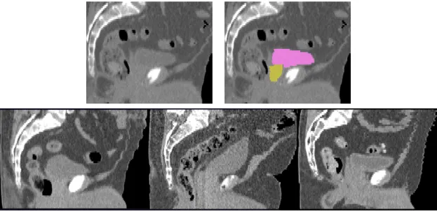
Figure 1.1: Top: Orthogonal slices of a 3D computed tomography (CT) image of the male pelvis, shown off-axis. Middle: Sagittal slice with bladder (blue) and prostate (green) segmentations. Bottom: Coronal view with corresponding segmentations. The red lines show the intersection of two orthogonal slices.

can be described as having simple topology, another class of methods that has proven highly successful is termed deformable model segmentation (DMS), where some geo-metric model is deformed to fit an image so that the deformed model is consistent with evidence for the object in the image. A subclass called Bayesian deformable model meth-ods is characterized by the use in optimization of (sometimes nominally) probabilistic terms that reflect the shape and appearance of the object of interest.

(14)

appearance in an object-relative and regional way. I have developed novel appearance models that extend such models and that are characterized by clustering and/or shift-ing on object-relative regional image descriptors. To justify object-relative appearance, consider that the shape model that fits the organ of interest may define a coordinate system on the image that is object-relative. This coordinate system has the advantage that anatomical relationships between the organ of interest and its neighbors are de-scribed more naturally than by using the simple voxel coordinates. Such anatomical relationships may vary from person to person and day to day. To justify regional ap-pearance, consider that an image can be decomposed into regions such as organs that are distinct from one another in their intensity characteristics. With these keys in mind, my appearance models for segmenting an object in an image useclustering to determine these regions and their intensity patterns and shifting to account for the variability in the object-relative position of these regions.

The remainder of this chapter is organized as follows. Section 1.2 reviews Bayesian deformable model segmentation and the objective function underlying such optimiza-tions. Section 1.3 describes image appearance models and posits the advantages of object-relative and regional models. The chapter concludes with the thesis statement, a list of accomplishments toward this thesis, and an overview of the remaining chapters of this dissertation.

1.2 Bayesian Deformable Model Segmentation

In Bayesian deformable model segmentation for medical images, a geometric model for an object of interest is initialized in an image and then deformed via its shape parameters

(15)

function is the posterior probability of the shape model parameters given the image data, arg maxmp(m|I).

Informally, consider an average shape of an object and some target image that in-cludes a particular instance of that object. Bayesian deformable model methods then look to deform the average shape as little as possible while fitting the particular object seen in that image as well as possible. The keys to this process are how to compute an average shape and measure the size of a deformation, which are aspects of shape, and how to measure the fit of a deformed model to the particular image object, which is an aspect of image appearance. These measurements are made using probability distribu-tions on shape and image appearance respectively. Often, the probability distribudistribu-tions are learned from a training set of previously-segmented cases of the same object and image modality.

The keys to the Bayesian process can be understood by applying Bayes’ formula to the posterior:

p(m|I) = p(m, I)

p(I) =

p(m)·p(I|m)

p(I) . (1.1)

In that p(I) is constant for any given image, the posterior p(m|I) is proportional to

p(m)·p(I|m), and thus

arg max

m p(m|I) = arg maxm [p(m)·p(I|m)]. (1.2)

(16)

arg min

m [−logp(m|I)] = arg minm [−logp(m)−logp(I|m)]. (1.3)

In the above equation the two terms−logp(m) and−logp(I|m) are penalties against low probability in the shape and image distributions respectively. This formulation is often used given the plethora of minimization schemes such as the gradient descent and conjugate gradient methods (Shewchuk, 1994). Additionally, in the case that the prior and likelihood are each given by a Gaussian model, the negative log cancels the exponen-tial of the Gaussian and the result is the square Mahalanobis distance (Mahalanobis, 1936), a popular and efficiently calculated statistical distance metric well-suited – in that it is quadratic – to the these minimization techniques.

In practice, the prior and likelihood probability distributions are often defined heuris-tically. Ideally however, they are trained given a set of previously expert-segmented cases in order to drive the optimization to expert-like results.

This dissertation focuses on the image match term and its underlying appearance models. The following section describes image match in more detail and presents male pelvis segmentation in computed tomography (CT) as motivation. Following that, I present my thesis statement and claims, and an outline of the rest of the dissertation.

1.3 Image Match and the Image Appearance

Mod-els

The image match term defines the fit of the deformed object to the image data; it is a result of the appearance model. An appearance model describes the grey-level intensity information relative to the object being segmented, typically relative to the object’s boundary.

(17)

the intensity within the disk is brighter than outside the disk, an effective appearance model would capture that information. Initial attempts considered the edge strength (gradient magnitude) of the image at the boundary of prospective disks. However, several image aspects common to medical segmentation make such a model inadequate. First, the presence of noise in the image misinforms the segmentation process as to the boundary of the disk. Adding to this is the fact that the entire boundary of the object in an image is not always characterized by a change in intensity. A better model might consider the average intensities inside and outside the disk. The average is an example of a parameterization of the intensity information taken with some aperture (here, the inside or outside). A resulting image match could be the difference between these inside and outside averages, and a prospective disk that maximizes this difference

(¯iinside−¯ioutside) would be a good segmentation. A problem with this match could be

that a collapsed disk containing only the brightest pixel in the image would maximize the inside/outside difference. However, recall that the shape prior would prevent this from happening were such a disk unlikely.

For a probabilistic image match in the same context, one could capture the average inside and outside intensities for a set of training images and fit some distribution (e.g., Gaussian) to them. The resulting image match could then be the joint probability of the inside and outside averages, i.e. p(I|m) = p(¯iinside,¯ioutside), where the prospective disk’s

shape parameters m (e.g., center and radius) define inside and outside. One subtlety here that is relevant throughout this work is that I have substituted a probability of I

given m with a probability of I relative to m. This assumes that regions in the same

(18)

as envisioned above will not be adequate for some applications such as pelvic organ segmentation in CT. Often a target object may have lighter and darker parts within itself, so a single number such as average intensity does not adequately characterize its appearance or the variation in appearance across images.

In the work I present here, I use two parameterizations that more completely de-scribe the intensity information. The first is termed profiles. A profile is a tuple of intensity sampled from inside to outside the object along the normal to a specified point on the boundary; profiles are obtained for many points on a single object boundary. A profile provides a very local description of the appearance across the object boundary at a point. The second parameterization, called a quantile function, records a function of the empirical distribution on intensity within a region. This function of the regional histogram has the attractive property that certain common changes in a distribution are represented linearly in the feature space (Broadhurst et al., 2006). Due to this lin-earity, quantile functions are amenable to Euclidean statistical methods (e.g., principal component analysis) for modeling the variation in appearance across images.

1.3.1 Object-relative, regional appearance

This subsection motivates the use of object-relative and regional image appearance mod-els.

(19)

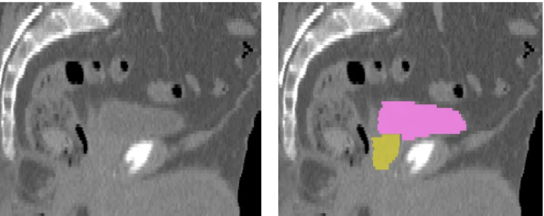
Figure 1.2: Sagittal male pelvis slices in CT. Top: Original greyscale image on the left, with bladder (pink) and prostate (gold) highlighted on the right. Bottom: Across images, note that the bladder is surrounded by mostly lower intensity bowel and fat, with much brighter tissue from the pubic bones and prostate inferior to (below) it. The prostate has a similarly consistent object-relative appearance. These observations motivate an object-relative regional appearance model.

there can be regions of similar intensity at corresponding places relative to the object geometry.

Consider the prostate as an example. A pelvic image including the prostate exists in a space in which the coordinates of a voxel are relative to the scanner. If the patient is imaged twice in differing positions relative to the scanner, then at the voxel coordinates where there is prostate in one image there may be no prostate in the other, and the images are completely different. This is because voxels with the same scanner-relative coordinates are assumed to be in correspondence. However, the images are identical if the voxels are sampled more naturally according to a coordinate system implied by the prostate geometry. For example, 2 cm superior to the prostate (toward the head) is 2 cm superior to the prostate in both images and will have about the same intensity.

To continue with the example, an appearance model can take advantage of this

(20)

the prostate, while the pubis bones, and their appearance, are anterior to (in front of) it. An effective appearance model in this situation will account for these differing expected intensities relative to the object. Determining the correspondence required for such an object-relative appearance model is a much larger problem than is completely addressed in this work (see (Davies et al., 2003; Cates et al., 2007) for a larger discussion on determining correspondence). For the appearance models described here, the initial correspondence is provided by the deformable model geometry, discussed later. For two models, that geometric correspondence is relaxed through shifting of the appearance model on the surface of the object model (see below).

A disadvantage of previous models is the use of “global” inside/outside regions. Global regions ignore the natural decomposition of the image space, especially in the exterior of the object of interest. Given the subject (a human body), medical images are populated by regions of relative homogeneity in tissue composition, which is reflected by homogeneity in the local intensity. Consider that what constitutes such a region is an organ or other volume whose local intensity distributions are distinguishable from those of neighboring volumes. In the example above the prostate is surrounded by regions of homogeneity that represent the bladder and pubis bones, rectum and neighboring fat deposits. These regions are a cause of intensity inhomogeneity in the organ exterior.

In this work I find regions through clustering on local intensity distributions. To avoid the infinity of possible regional shapes and positions, the regions are constrained to be on the boundary of the object of interest and extended normal to the boundary, inside or outside.

The variability in the positions of these regions is also lost on global appearance mod-els. At the same time, the sliding of neighboring regions with respect to one another and the object of interest cause problems for methods that assume a voxel scale correspon-dence (see Chapter 2). Two of the image matches I propose in this work use shifting

(21)

positions of these regions.

1.4 Thesis

Thesis: The automatic segmentation of medical images via deformable

models benefits from the use of object-relative, regional statistical appearance

models. Specifically, clustering on either local or regional object-relative

im-age descriptors can provide an effective understanding of the context of the

object of interest in the image. Additionally, the use of shifting to account for

the variability in the position of object-relative regions allows for relaxation

of the geometric correspondence provided by the deformable model and often

leads to improved segmentations.

1.5 Claims

Contributions included in this dissertation are as follows:

1. I demonstrate that clustering on local image descriptors can be used to construct effective appearance models for deformable model segmentation.

2. I present a novel appearance model and image match using clustering on intensity profiles that reflects the various edge characteristics in the image boundary region. This model leads to improved kidney segmentation in CT versus a previous image match.

3. I demonstrate that regional intensity quantile functions (RIQFs) are a more effec-tive local image descriptor than intensity profiles.

(22)

and prostate segmentation in CT.

5. I demonstrate that the object-relative positions of neighboring organs and volumes change across images, leading to a false association of image regions due to the geometry-implied correspondence.

6. I present two novel appearance models and associated image matches that account for this variability in the external conformation of neighboring regions through shifting of the image model on the object boundary. The two models differ in the scale of the regions undergoing shifting. These models often lead to improved segmentations over those achieved using their static counterparts. I validate this by experimentally testing the efficacy in segmentation of these appearance models on bladder and prostate in CT.

1.6 Overview of the Chapters

This dissertation is organized in six chapters, with this chapter introducing and moti-vating the work. The remainder of the dissertation is organized in the following:

Chapter 2 provides a review of previous image matches and Bayesian deformable model segmentation in general. Also presented is an introduction to the deformable model of choice in this work, the discrete medial representation, or m-rep. Finally, this chapter reviews in more depth the image descriptors used in this work, intensity profiles and regional intensity quantile functions.

(23)

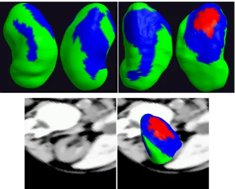
Chapter 4 presents a comparison of appearance models at three object-relative re-gional scales from global to local. This chapter also presents an appearance model and image match based on a static decomposition of the object boundary and clustering on local RIQFs. After determining region types through clustering, the method partitions the object boundary according to region type and captures the intensity variability per region type using principal component analysis (PCA). This model’s efficacy is evaluated on bladder and prostate segmentation in CT.

Chapter 5 presents two appearance models and their associated image matchs that improve upon the models of Chapter 4 by allowing the region-type partition on the boundary to slide according to variability in the partition seen in training. The changing in the partition is accomplished using an iterative process. The image matches are also validated in this chapter, on bladder and prostate segmentation in CT.

(24)

Chapter 2 Background

Appearance models and the resultant image matches are an integral part of all automatic segmentation schemes. They define the fit of a prospective segmentation to the image data and thus are required for any optimization to take place. The appearance models I have developed in this dissertation can be better understood within the context of previous models. In this chapter I present a survey of appearance models and discuss their strengths and weaknesses.

I classify appearance models according to the scale of the image match computation.

Voxel-scale models consider the image information at the level of individual ordered

voxels1_. _Region-scale _{models consider information over many voxels at once (e.g., the} intensity distribution in the interior of the object of interest). Within these two cat-egories, I further classify appearance models according to whether the model encodes variability in appearance: models are either static or probabilistic.

1_{While I usually refer to the image information as intensity, which is most common in the literature}

(25)

2.1 Voxel-scale Models

The simplest voxel-scale model assumes that the object edge corresponds to a local maximum in the image gradient magnitude (Canny, 1986). The active contour and “snake” segmentation methods of (Kass et al., 1988; Caselles et al., 1997) both use this idea, attenuating a local growth force on the shape model according to a function of the local gradient such as magnitude. The overall image match is then proportional to the integral of this local match over the whole contour S,

p(I|m)∝

I

f(∇I(S(u)))du. (2.1)

(Cootes et al., 1995) also use an edge strength image match within the context of the notable Active Shape Model segmentation scheme (see below). Here, the authors use the derivative of the intensity profile at an object boundary point to determine the displacement of that point along its normal. In the work of (Staib and Duncan, 1992), the edge strength image match is paired with the Fourier-parameterized boundary model.

(26)

2.1.1 Static template methods

Several approaches have been proposed to account for the differing appearance around the object. Some methods use the appearance from a single example image to cre-ate a static templcre-ate to match against at target time. Examples of this are found in the medially-based deformable model segmentations of (Pizer et al., 2003) and in the diffeomorphic image warping of (Miller et al., 1999).

In (Pizer et al., 2003; Joshi et al., 2001), the medial representation, or m-rep shape model is used within the Bayesian DMS framework (see Chapter 1). In this scheme, intensity profiles are sampled for a collar region about the boundary of the shape that fits a single expert-segmented image. The collection of profiles is termed a simple mask, in that it is trained on only one image. At target time, the corresponding profiles are sampled for the prospective shape in the new image. The image match is then normalized correlation of the target profiles with the profiles from the training case:

p(I|m)∝X·T, where X is a column vector formed by the concatenation of the target profiles and T is that from the training case. In an approach that mimics the gradient magnitude image match above, the training profiles can be substituted with profiles that encode an intensity step edge from inside to outside, implying a bright object on a dark background or vice versa. An improved image match using the profile descriptor is the subject of Chapter 3. The m-rep shape model is covered later within this chapter (see Section 2.4), as my image matches also use the object-relative correspondence it provides.

(27)

corresponding voxel intensities in the deformed template and the target,

p(I|m)∝

I

Ω

|T(x−u(x))−S(x)|2_dx, _(2.2)

whereuis a displacement field,T is the template image andS is the target. Davis et al. use this scheme to perform regression on ordered images and construct a moving average image, such as the aging brain in MRI (Davis et al., 2007; Davis, 2008). Regional and probabilistic image matches in the image registration literature are covered below.

Mutual information is another image match popular particularly for the registration of images of different modalities (Maes et al., 1997). Here, as in the above, the purpose is to determine a warp (here constrained to be affine) that deforms the template image to fit the target. The mutual information (M I) image match is entropy based, essentially measuring the degree to which the two images arenot independent; that is, how well a voxel in the deformed template image predicts the value of the corresponding voxel in the target. Seen one way,M I measures the difference between the sum of the individual entropies of the two images, seen as random variables X and Y, and the joint entropy:

M I(X, Y) =H(X) +H(Y)−H(X, Y). (2.3)

For another way to think of mutual information, consider that pX(x) and pY(y) are

the marginal distributions of X and Y and pX,Y(x, y) is the joint distribution, all as

histograms for example. If X and Y are independent, then the joint distribution is equal to the product of the marginals: pX,Y(x, y) = pX(x)·pY(y). M I then measures

the degree to which the product of the marginals is not the joint, using the Kullback-Leibler divergence between the joint and the product of the marginals,

M I(X, Y) = X

x,y

pX,Y(x, y)log

pX,Y(x, y)

pX(x)·pY(y)

(28)

(Studholme et al., 1999) construct a normalized MI measure, the ratio of the sum of the individual entropies and the joint, that they claim improves the robustness of registration under certain conditions. (Gan and Chung, 2005) also claim improved registration using

M I on a feature vector including both the traditional intensity and what amounts to a smoothed gradient magnitude. (Tsai et al., 2004) propose a mutual information-based active contour segmentation where the image match is the mutual information between the target image intensities and the prospective segmentation labels, as opposed to the template image intensities.

2.1.2 Probabilistic methods

The static template models were devised to account for the differing appearance around the object. However, being trained on a single example case, they capture limited infor-mation. Among sets of images, there is additional variability even among anatomically corresponding voxels. Several probabilistic, still voxel-scale models have been proposed to account for this variability. These probabilistic appearance models lead to optima with the most statistically likely image characteristics rather than optima most like a single arbitrarily chosen training case.

(29)

target profile in its respective distribution. Kelemen et al. use this PCA-per-point ap-pearance model on the original grey-scale intensity profiles. Their work is in the context of deformable model segmentation with the spherical harmonics shape model (Kelemen et al., 1999).

Many statistical appearance models assume for practicality that the elements of a feature vector such as a profile are independent. This assumption may not be ideal, in that the samples forming the profile are highly spatially correlated and thus some correlation in the intensity can be expected. Duta et al. (1999) present another prob-abilistic, profile-based appearance model, but in this case partially accounting for the correlation by modeling the profile as a Markov chain. The purpose in this case is to detect places in the target image that are statistically likely to be the object of interest, given training. The scheme involves sampling a small number of intensity profiles at a fixed number of positions through a square region of the image. The concatenated profiles form the feature vector for that region. The feature vectors sampled over all positions within all training images form two populations, those vectors corresponding to positions that were in the object of interest and positions that were not; positive and negative examples respectively. The method then determines a maximally discrimina-tive Markov chain model for the feature vectors of the two populations. At target time, positions are classified as the object of interest if the log-likelihood ratio exceeds some threshold T:

L(x) = log P(x)

N(x) > T >0, (2.5) wherexis the position’s profile in the target image–the target feature vector–andP and

(30)

the direction of the normal to the boundary at that point. The method considers the set of feature vectors sampled at a corresponding point across training. In that the original active contour methods do not require correspondence–the edge-strength model is the same regardless of position along the boundary–the correspondence here is provided by the user and by preprocessing alignment steps. The intensity and directional derivative of the feature vector are each modeled with a Gaussian distribution. At target time the image match of a prospective segmentation is the Mahalanobis distance of the target feature vector, integrated over the contour S. That is, p(I|m)∝e−EI_{, where}

EI = I

(I(S(u))−µI)2

σ2

I

du+

I

(S⊥(u)· ∇I(S(u))−µ∇)2

σ2

∇

du (2.6)

(31)

For a particular blurring level, the goal is to model the target image in terms of the warping parameters t to the average shape, the coefficients con the modes of the PCA model on intensity, and intensity normalization parametersu. The image match is then simply the sum of squared differences between the actual target image and the modeled target. The authors further devise a scheme for analytically determining the change in

pT = (cT|tT|uT) required to improve this image match. (Scott et al., 2003) extend the AAM framework by considering not only the intensities but also image filter responses that encode local texture and geometric information, replacing a single intensity at each pixel with a “local structure tuple.”

There is additional segmentation literature focused on classifying each voxel in an image (Gerig et al., 1992; Priebe et al., 2006; McLachlan et al., 1996; Woolrich et al., 2005; Duda et al., 2001; Jain et al., 2000). These schemes use training cases to model the classes of tissue being segmented, usually using Gaussian or mixture of Gaussian distributions. Though they also often involve the use of regularizing and spatial prior techniques to limit the noise in the classification, they can still be considered voxel-scale. Voxel-scale models are characterized by an understanding of the image appearance at the most local scale, whether as local gradient information, per-voxel differences, or distances and statistics on ordered collections of points. They rely on a voxel-scale correspondence between training and target and across training cases. These schemes are effective in situations where objects of interest and their surroundings have a consistent voxel-scale relationship with one another.

(32)

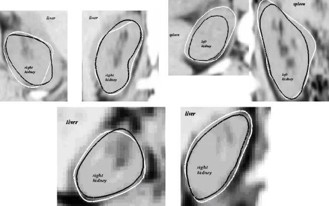
Figure 2.1: Corresponding coronal CT slices of two human abdomens. The liver, in the upper left of each patient image, has a widely disparate correspondence with the nearby kidney. This variability poses a challenge in constructing an effective image match function for prospective kidney segmentations.

However, in the abdomen there is large variability in the pose of organs relative to one another, and thus in the observed appearance, in that the organs are essentially floating (see Figure 2.1). Thus for example, an effective kidney segmentation depends on both the appearance of points interior to the kidney and also the appearance of the non-rigidly related and perhaps distorted configuration of objects near the kidney, such as liver and rib and fat.

2.2 Region-scale models

(33)

2.2.1 Static template methods

The static template methods are those that match against a single exemplar or training case. In the image registration literature, normalized cross-correlation is a popular regional, static-template image match (Zitov´a and Flusser, 2003; Pratt, 1991). Recall that the goal is to determine a warp that deforms the template image to fit the target. Normalized cross-correlation (CC) is used to find corresponding (usually square) regions between the images. If X and Y are the intensities within a pair of windows, one each from the target and temple, then the normalized CC is given by

CC(X, Y) = _p E((X−E(X))(Y −E(Y)))

E((X−E(X))2₎p

E((Y −E(Y))2₎, (2.7)

where E(·) is the expectation value or mean. CC amounts to the dot product of the windows after normalization. By finding corresponding window pairs in the images, the warp aligning the two images can be determined. While there is extensive variation in the warping model itself (Maintz and Viergever, 1998; Zitov´a and Flusser, 2003), the image registration literature provides a variety of image matches based on sum of squared differences, cross correlation, and mutual information.

Regional approaches most often model intensity distributions in object-relative re-gions, as opposed to the windows seen above. For example, the “region competition” extension to the classic active contour segmentation scheme considers the intensity dis-tributions on the interior and exterior of the object of interest (Zhu and Yuille, 1996). In this method the local force applied at a point~v on the contour is determined in part by the log-likelihood ratio of the intensities near that point,

logp(I~v|αint)−logp(I~v|αext), (2.8)

(34)

near ~v. The authors model the interior with a Gaussian — αint = {µ, σ2}, and they

model the exterior with a uniform distribution. (Yushkevich et al., 2006) claim improved results in two steps; first, rejecting the log ratio and instead using a simple difference in probabilities; and second, modeling the interior with an intensity range and two-sided smooth threshold filter and the exterior as merely the complement of the interior,

p(I~v|αext) = 1−p(I~v|αint).

In addition to mean and variance or intensity ranges, there are many possible param-eterizations of the regional intensity distribution. To this end, (Tsai et al., 2003) extend the work of (Chan and Vese, 2001) within the context of a level set-based segmentation scheme. The authors propose a gambit of regional image statistics in addition to the mean and variance, including the sum of the intensities and the sum of the squared intensities within a region. The regions in this work are the interior and exterior.

In these works, the template values are simply those image statistics for the current interior and exterior regions. The image matches or image energies described are of several types. In one example (Chan and Vese, 2001), the energy to be minimized measures the discrepancy between the inside intensities and the inside average and also the outside intensities and outside average:

Ecv = Z

Ru

(I −µ)2dA+

Z

Rv

(I−ν)2dA. (2.9)

In this example, Ru _and _Rv _{represent the interior and exterior regions and}_µ_and_ν _their

respective average intensities.

(35)

maps.

Mean and variance and the other image statistics of (Tsai et al., 2003) are exam-ples of parametric representations of the underlying regional intensity distributions. In that these low dimensional parametrics often cannot adequately represent the nuances of the observed distribution, they are simplifications that can limit the information cap-tured by the appearance model. Some recent methods construct a static template image match using a non-parametric approach, modeling with a histogram the full intensity distribution for a region. These approaches require a means of comparing the template histogram with that observed at target time, analogous to the measurement of discrep-ancy in the image matches that use parametric statistics. Rubner et al. (2001) review and benchmark a number of these histogram matching functions with regards to classi-fication, image retrieval, and segmentation (additional metrics can be found in (Duda et al., 2001)). Let q and r be discretized intensity distributions (histograms) between which we wish to measure the similarity, and letQ and R be the respective cumulative histograms (CDF’s). Example histogram matches are found in the following table.

Name Equation Description

Minkowski-form Lp(q, r) = ( P

i|q(i)−r(i)|p)1/p Lp norm

Kolmogorov–Smirnov Dp₍_{Q, R}_{) = max}

i|Qp(i)−Rp(i)| max discrepancy on CDF

Cramer/von Mises Dp₍_{Q, R}_{) =} P i(Q

p₍_i₎₋_Rp₍_i₎₎2 _{square distance on CDF} Kullback-Leibler KL(q, r) = P

iq(i) log q(i)

r(i) summed log-likelihood

Rubner et al. (2001) also note the Earth mover’s distance (EMD), which defines the work required to transform one histogram into another, as a powerful measure. The EMD is equivalent to the Mallow’s distance metric used in the quantile function work of Broadhurst (Broadhurst, 2008). Quantile functions will be covered in some depth within the context of histogram matching functions in Section 2.3.1.

(36)

dis-tributions, but they also consider these distributions as a function of distance from the boundary. They explicitly train the joint probability relating image intensity to signed distance from the boundary of the object of interest. They do this by using a signed distance map as their shape model and by learning the joint distribution on intensity and signed distance over a number of training cases. At target time, the image match at a place in the image is proportional to this joint probability. The algorithm locally iter-ates the signed distance map (prospective segmentation) so as to optimize an objective function including this image match.

The appearance models presented above, using cross correlation, image statistics, and histogram matching functions, model the variability in the intensity of a voxel within the region. However they do not account for the variability in the regional distribution itself. It is in that sense that the appearance models described above are termed static. Particular instances of a region, such as the interior of an organ, may have a different mean and variance, for example, whereas those methods will always search for the exemplar.

2.2.2 Probabilistic methods

There are a few region-scale image appearance models in the literature that explicitly reflect knowledge of the training population in computing a match. There are two principal approaches to this. One is to relax the static template by allowing the match to be obtained against any (or some combination of) the training exemplars. The other approach is to measure the fit of the observed regional appearance using a probabilistic distance.

(37)

objects relative to the object of interest destroy this correspondence. The author relaxes the voxel-scale correspondence by constructing a profile scale space, a multiscale image match that uses blurring of the training profile data along the boundary of the object in order to disburse the local appearance around the object. At target time then, the segmentation scheme uses this multiscale model to provide a more robust localization of the object than the single scale profile model can produce.

Costa et al. (2007) propose a regional scale image match that fits against a template that changes through the course of the segmentation; this is an example of the first approach. The last level of the segmentation scheme is a deformable model stage that attempts to fine tune the mesh model result of the previous registration and morpholog-ical operations. The authors use as their initial template the histogram of the interior of the model resulting from the previous stages. The local force applied to a vertex s

of the mesh is determined in part by the whether image intensities at s are compatible with the current template histogram:

I(s)−µ σ

≤2 (2.10)

This is the absolute value of the standard or “z” score. As the mesh is deformed, the histogram of the interior changes and that changed histogram becomes the template used in further deformation. This scheme uses a region-scale appearance that is probabilistic in that it isnot static, in that the mean and variance of the particular instance is allowed to be different from what might otherwise be a static template2_.

The method of Costa et al. (2007) is like those of (Tsai et al., 2003; Chan and Vese, 2001) in that it uses low dimensional parametrics (mean and variance here) that often cannot adequately represent the observed distribution. Freedman et al. (2005) propose a “cdf distance” to match thefull intensity distribution observed at target time against

2_{Under this understanding of a probabilistic match, the works of Chan and Vese (2001) and Tsai}

(38)

that learned in training. The authors similarly only concern themselves with a single region, the interior of the object of interest. If q is the discretized intensity distribution (histogram) observed for a prospective segmentation and r is that learned in training, and if Q and R are the respective cumulative distribution functions (CDFs), the cdf distance is given by

K(q, r) =

n X

i=1

|Qi−Ri|α, (2.11)

for some power α > 1. As in (Tsai et al., 2003) above, the optimal segmentation is found by differentiating this image match with respect to the shape parameters, which are here the variational implicit surfaces of (Turk and O’Brien, 1999). As with (Costa et al., 2007) above, this scheme is probabilistic in the sense of the first approach. The particular training histogramrused to match against can change during the optimization to be any one of the histograms observed in training, whichever one is closest to the observed histogram q. A further complication is that the training histograms are not of the entire interior region in training, but rather random sub-regions within the interior. This approach is in the vein of nearest neighbor methods common in image classification if one thinks of the training histograms and the target histogram as existing in some space defined by the cdf distance.

2.3 Quantile functions and probabilistic region-scale

appearance

(39)

in the appearance modeling and image match literature. The quantile function is a distribution-based regional image descriptor that has advantages over other representa-tions, such as the histogram or CDF. The appearance models I present in Chapters 4 and 5 both depend on this representation of the regional intensity distribution and its amenability to the statistical models I use. In this section I review the quantile function construction and probabilistic image match methodology, which can be found in more detail in Broadhurst’s thesis (Broadhurst, 2008) and in (Broadhurst et al., 2005, 2006).

2.3.1 Regional intensity quantile functions

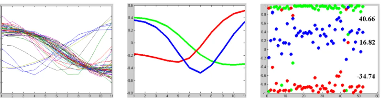
Regional intensity quantile functions (RIQFs) are an image descriptor that allows one to probabilistically represent the appearance of an object in an image. Quantile func-tions are derived from intensity histograms within object-relative regions, such as the interior near the object boundary. The space of RIQFs has the advantage that certain common changes in a distribution, such as mean shift and intensity scaling, are rep-resented linearly under a Euclidean metric. Principal component analysis is then used to characterize the variability in a set of quantile functions, and thus in the underlying appearance.

In the following I review the construction of the RIQF in the context of the distance metric that provides linearity. Letq and r be the continuous, one-dimensional intensity distributions in two regions between which one wishes to measure the similarity. As summarized above, (Freedman et al., 2005; Rubner et al., 2001) have proposed a number divergence measures for just this task. The Earth Mover’s Distance (EMD) is one such measure that is particularly intuitive. The EMD measures the work required to transform q to r by considering the distributions as piles of dirt: the work required is the amount of dirt times the distance that it must be moved.

(40)

−4 −3 −2 −1 0 1 2 3 4 5 6 0 0.05 0.1 0.15 0.2 0.25 0.3 0.35 0.4 x f_x

φ(0, 1) φ(2,1)

0 0.1 0.2 0.3 0.4 0.5 0.6 0.7 0.8 0.9 1

−3 −2 −1 0 1 2 3 4 5 Quantile x

−8 −6 −4 −2 0 2 4 6 8

0 0.05 0.1 0.15 0.2 0.25 0.3 0.35 0.4 x f_x

φ(0, 1) φ(0, 4)

0 0.1 0.2 0.3 0.4 0.5 0.6 0.7 0.8 0.9 1

−6 −4 −2 0 2 4 6 Quantile x

Figure 2.2: A standard normal distribution (blue), as probability density function (left column) and quantile function (right column) undergoing a mean shift and variance scaling (dashed green). Top row: mean shift. Bottom row: variance scaling. These changes are linear in the quantile feature space.

R respectively, the Mallows distance is defined as

Mp(q, r) =

Z 1

0

|Q−1(t)−R−1(t)|pdt

1/p

. (2.12)

An n-dimensional RIQF is then the discretized inverse cumulative distribution on intensities in a region, i.e.,Q−1₍_t_{) or}_R−1₍_t_{) in the above equation. Let these discretized} quantile functions be denoted q or r. Coordinate j of q or r stores the average of the [j−_n1,_nj] quantile of the intensity distribution for that region, i.e,

qj =n

Z j/n

(j−1)/n

(41)

The Mallows distance above corresponds (up to a scale factor) to the Lp vector norm

between qand r,

Mp(q, r)≈

1

n

n X

j=1

||qj−rj||p !(1/p)

. (2.14)

In the above, given a sample of data the quantile function is constructed through computing the histogram of the sample and then the corresponding inverse cumulative distribution function. I take another, equivalent approach throughout this work in my construction of the quantile function. In my work, a weight with a maximum value of 1 is associated with every sample. Using a constant weight of 1 is equivalent to having the samples unweighted. Consider a list of data/weight pairs with a total weight of

N, {(di, wi)| P

wi =N}, and a goal of constructing the associated quantile function of

length n. After sorting the data such that di ≤dj,∀i < j, the elements of the quantile

function (the quantiles) are the weighted averages of consecutive sections of the sorted list. The number of data samples in each section can be different, as long as the sum of the weights in each section is N/n. For example, the first quantile is n

N P

iwidi, where

i is such that P

iwi =

N

n. If N does not divide evenly, then some data samples will

contribute to multiple quantiles. In the case where N < n, a sample could contribute to more than two consecutive quantiles.

Through the use of intensity quantile functions, distributions are understood as points in an n-dimensional Euclidean space in which distance corresponds to the M2 metric. Furthermore, the discretized quantile function of a distribution has advantages over other representations in that some important changes are represented linearly in this space. Namely, a shift in the mean or scaling of the variance are both linear changes in the quantile function space. For example, theM2 distance between Gaussian distributions N(µ1, σ21) and N(µ2, σ22) is

p

(42)

2.3.2 Principal component analysis (PCA)

Principal component analysis (PCA) is a technique for determining modes of variation in Euclidean data and can be used to construct a probability distribution on such data. It basically finds orthogonal directions of greatest variance in the data. It is the singular value decomposition of the covariance matrix Σ, and in general solves the equation Σ~x = λ~x, where the satisfying λ and ~x are termed eigenvalues and eigenvectors of Σ respectively. Consider a sample of m n-dimensional points, ~xi ∈ <n. The matrix

X = [~x1. . . ~xm] records this sample. If ~µis the row-wise mean ofX (which is a column

vector), then the covariance matrix is given by the outer product

Σ = 1

m(X−~µ)(X−~µ)

T

(2.15)

IfV = [~e1. . . ~en] is the collection of eigenvectors andD=diag([λ1. . . λn]) is the diagonal

matrix with associated eigenvalues, then Σ·V =V ·D. Furthermore, if the original data are Gaussian distributed,X ∼N(~µ,Σ), then~eT_i (X−~µ)∼N(0, λi) and we can model the

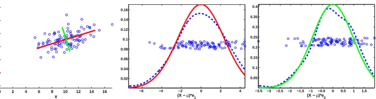
data accordingly. That is, the mean-normalized data projected onto theith eigenvector follows a normal distribution with variance equal to theith _{eigenvalue. Figure 2.3 shows}

an example of PCA on 2D data. The resulting Gaussian model is overlaid on the data. The above all assumed that the sample size was greater than the dimension of the data. Given m < n points in <n_{, PCA can recover only} _m₋_{1 modes. This is}

accom-plished by setting Σ to the inner product _m1(X−~µ)T₍_X₋_~_µ_{) and setting the resulting}

V = (X−~µ)·V.

(43)

0 2 4 6 8 10 12 14 16 −2 0 2 4 6 8 10 x y

−6 −4 −2 0 2 4

0.02 0.04 0.06 0.08 0.1 0.12 0.14 0.16

(X − µ)*e1

−3.5 −3 −2.5 −2 −1.5 −1 −0.5 0 0.5 1 1.5

0.05 0.1 0.15 0.2 0.25 0.3 0.35 0.4

(X − µ)*e2

Figure 2.3: An example of principal component analysis on random 2D data. Left: scatter plot showing the data (blue) with±2σ in the principal directions plotted about

~

µ(red and green respectively). Middle: the data projected onto the first principal mode,

~e1, with a kernel density estimate (dashed blue) and the captured modelN(0, σ21) (red). Right: projection onto ~e2.

of V, we have the equalities:

~x0 = ~µ+V ~c0 (2.16)

~c0 = VT(~x0−~µ), (2.17)

where~c0 is the set of coefficients on the eigenvectors. Modeling the data as a Gaussian, we have

p(~x0) =

1

(2π)n/2_|Σ|1/2exp

−1

2(~x0−~µ)

T_Σ−1₍_~_x 0−~µ)

. (2.18)

With the data projected into the pca space via (2.17), the data covariance Σ becomes the diagonalD and the computation becomes much easier.

(44)

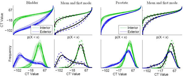
Figure 2.4: Training intensity distributions as quantile functions (top row) and his-tograms (bottom row). Bladder and prostate over all images of a single patient (Broad-hurst et al., 2006). The regions represented are the near interior and near exterior.

shift and variance scaling, which are linear operations in the RIQF feature space.

2.4 The m-rep deformable shape model

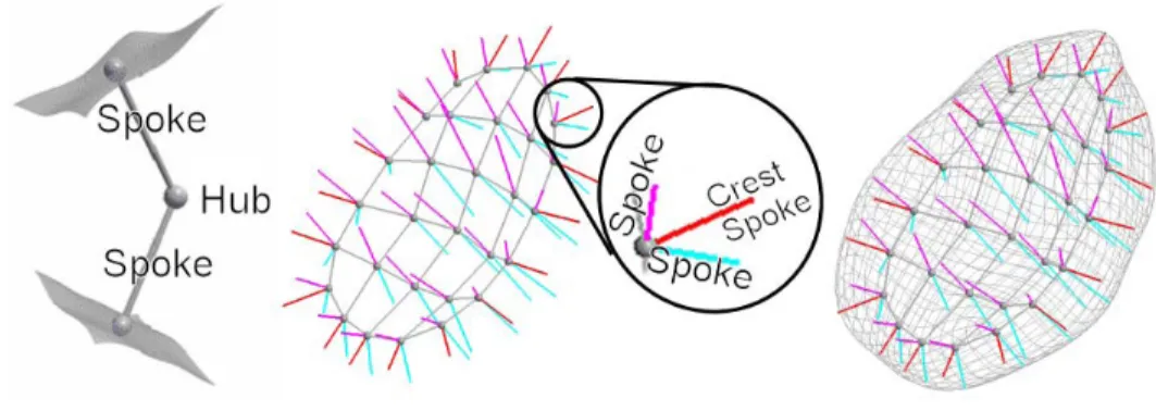
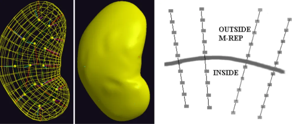
The appearance models I develop in this dissertation are tested within the context of automatic segmentation by the posterior optimization of m-reps. This section describes the m-rep shape model and its use in Bayesian deformable model segmentation. The “m-rep”, or discrete medial representation, is a skeletal geometric model used to describe the shapes of bladders, prostates, rectums, and kidneys (Joshi et al., 2001; Pizer et al., 2003, 2005a), and one can also model more complex shapes using collections of m-reps (Han et al., 2005). An m-rep is a discretely sampled grid of medial atoms, where each atom consists of a hub and two equal-length spokes. The boundary of the object model passes orthogonally through the spoke ends (see Figure 2.5).

(45)

Figure 2.5: A medial atom, a discrete m-rep, and the implied boundary for a bladder.

Figure 2.6: Two instances of a bladder m-rep and surface with corresponding region highlighted.

While this correspondence has proven effective when there are appropriate constraints on the deformations allowed of the model (Han et al., 2007; Merck et al., 2008), the correspondence may not be appropriate for all purposes.

The surface is a derived property of the m-rep, with the points on the surface com-puted deterministically from the medial grid. This leads to a constructive approach to sampling an image relative to an object, stepping along profiles normal to the surface that are also provided by the m-rep. The image regions of concern are found close to the boundary of the object of interest, as it is these regions that inform where the boundary should be.

(46)

m-reps. See Section 1.2 for a more general introduction to Bayesian deformable model segmentation. To start, a mean model (in some sense an average shape) is positioned in a target image using a similarity transform that may be computed from a few landmarks or a hand-placement or may be based on bone registration. After initialization, we optimize the posterior p(m|I) of the geometric parameters given the image data. This is equivalent to minimizing the sum of the negative log-prior logp(m) and negative log-likelihood logp(I|m), which measure geometric typicality and image match, respectively. Geometric typicality and the initial mean models are based on the statistics of m-rep deformation over the training set Fletcher et al. (2004). This “principal geodesic analysis” is analogous to PCA, but on manifold rather than Euclidean data. The image match model comes from some appearance model, whether it is the template profile match described in Chapter 3 or the result of applying PCA to the set of RIQFs sampled from the m-rep training set, as is the case in the later chapters. A limited number of modes is used to avoid numerical problems and because a small number of modes is enough to describe the vast majority of variability in the data.

To compute the image match of a prospective segmentation (a given m-rep), we first sample the regions relative to the m-rep to construct the regional histogram and the resultant RIQF. The image match term is then the negative log of (2.18) after projection into the PCA space via (2.17). If ~c0 is the PCA coefficients of the RIQF observed for a region, then

−logp(I|m) =~cT₀D−1~c0 (2.19)

The right-hand side~cT

0D

−1_~c

(47)

computed over all regions (such as interior and exterior) and the results added together for the final match.

2.5 Validation

In order to test the effectiveness my image matches, I have relied on their efficacy in segmentation tasks. I compare automatically obtained m-reps models against expert manual segmentations, which come in the form of binary images. To perform this comparison, one can either rasterize the m-rep model in order to compare directly against the binaries, or one can tessellate the boundary in the binaries and compare surface to surface. The tessellation can be accomplished using the Marching Cubes (Lorensen and Cline, 1987) technique to find the boundary isosurface in each binary image (which should be slightly blurred to smooth the voxelization). In choosing to compare surface to surface, I have developed a tool for comparing two closed surfaces called compare byu (the surfaces are provided in the byu tile file format). This tool computes metrics such as volume overlap and closest point surface-to-surface distance in the vein of the published Valmet tool, which only compares binary images (Gerig et al., 2001). In this subsection, I will discuss validation metrics and specifically this tool and its computation of chosen metrics.

(48)

Figure 2.7: Left: The surface distance from A toB is not the same as that from B to

A. Right: Schematic of the orthographic ray projections used to calculate the volume overlap. The cyan ray extents represent intersection volume, while the blue and dashed green extents represent volume exclusive to A and B respectively.

The closest point distance from a vertex a on one surfaceA to the other surface B

is computed as the minimum over all triangles of B of the point-to-triangle distance from a (Eberly, 1999). This value is averaged over all vertices on A to obtain ASDAB

and its maximum is taken to obtain the Hausdorff distance from A to B. Note that

ASDAB 6= ASDBA, that is ASD is not symmetric. This is seen in that the minimum

distance from the vertex a to surface B is traversed along the normal of the surface B

at the corresponding point b while the closest point on surface A from b will involve a normal of A, and these normals only line up if the surfaces are locally parallel (see Figure 2.7). If A is the automatically obtained surface and B is the manual reference, then ASDAB may be chosen over symmetric measures (like the average of ASDAB and

ASDBA).

(49)

the 95th _{percentile of the minimum distances observed from} _A _to _B_{. In that same line}

there may be an advantage to considering the entire distribution on minimum distances, rather than such single values as mean, median, 95th _{and other percentiles (the median}

is the 50th_).

Volume overlap gives another performance measure, this for the degree to which the interiors of the two surfaces match up. IfA and B now represent the volumes enclosed by the respective surfaces, then the most common volume overlap measure is the Dice similarity coefficient (Dice, 1945), measuring the intersection divided by the average:

DV(A, B) = 2 ||A∩B||

||A||+||B|| (2.20)

I compute this measure between the two surfaces using a constructive solid geometry approach–a French fry method. Intuitively, consider an x-y parallel plane that is below the two surfaces, the bottom of the bounding box for example. A ray normal to the plane that extends upward will intersect the surfaces at some heights. As one moves along the ray, depending on which surfaces have been intersected and how many times, one adds bits of volume to||A||, ||B||, and/or ||A∩B|| (see Figure 2.7). As long as the resolution of the rays on the plane is smaller than the triangles making up the surfaces, then these French fry volumes along a ray can be approximated with rectangular prisms. For speed and robustness, the actual implementation involves orthographic projection onto the three planar axes and averaging of the results.

(50)

(51)

Chapter 3 Intensity Profile Clustering on

Image Boundary Regions

In deformable model segmentation the image match can be thought of as measuring the degree to which the target image conforms to some template within the object boundary regions (see Section 1.3). The template should account for variation over a training set and yet be specific enough to drive an optimization to a desirable result. Some templates imply a constant appearance near the boundary, which is too general, while others model the appearance at each point separately, which while more specific is subject to sampling noise. In this chapter I present a novel approach to reflect the appearance changes near the boundary while lessening the sensitivity to noise of the fully local approach1_{. This method uses clustering on local intensity profiles. The method groups} the appearance over many points to come up with point appearance types that robustly characterize image intensity in object boundary regions. The appearance model I present is an example of a voxel-scale, static-template model (Section 2.1.1). My method first determines local cross-boundary image profile types in the space of training data and then builds a template of optimal types. This chapter also presents results from the application of this method to kidney segmentation in CT, showing improvement over a

1_{The work presented in this chapter appeared in Stough, J., Pizer, S., Chaney, E., and Rao, M.}

(2004). Clustering on image boundary regions for deformable model segmentation. In IEEE

(52)

previously built model (Rao et al., 2005).

3.1 Introduction

As discussed in chapter 2, deformable model segmentations proceed based on the op-timization of an objective function that includes a term measuring geometry-to-image match (image match, for short) giving the likelihood of the model with respect to the image information. The likelihood function is often trained on a set of ground truth segmentations in order to drive the optimization to expert-like results.

Among voxel-scale models (Section 2.1), several previous methods involve the use of intensity profiles as a local image descriptor. A profile is an n-tuple of intensities sampled from an image in some fixed geometry-relative way. A profile can thus be seen as a point in an n-dimensional feature space.

Previous work on building the likelihood function have included intensity profiles associated with individual image points (Cootes et al., 1995), full images referenced with a coordinate system defined by a collection of these points (Cootes et al., 1999), and intensity profiles and structure information associated with a tiled boundary (Mon-tagnat and Delingette, 1998; Fenster and Kender, 2001). The methods typically make assumptions of a unimodal probability distribution of corresponding intensity profiles, and two of them train for each point separately. In our experience the distribution is often widely variable and multimodal, leading to concerns in the ability to model the intensity at each point by the family of training images at that point alone. To address this concern, one may choose to model the appearance at all points equally, as in look-ing for strong edges (Canny, 1986). This approach is oversimplified however, given the context of organ appearance in medical images.

(53)

Figure 3.1: The right kidney highlighted in both axial (left) and coronal CT slices. Note the variable intensity pattern with respect to the kidney.

Figure 3.2: Left: the m-rep model shown as wireframe and surface. Right: diagram of closeup of the m-rep surface showing profiles, which sample intensity from inside to outside the m-rep along the normal to the boundary.

that is stable against image variability and effective in measuring image match can be made from local image descriptors that are representative of those observed in training images. As a local image descriptor, I use intensity profiles that are generated along normal directions to the densely sampled model boundary (Figure 3.2).

Clustering and shifting of regional appearance for deformable model segmentation