Advance Access publication on June 20, 2016
Prediction of cancer drug sensitivity using
high-dimensional omic features
TING-HUEI CHEN
Department of Mathematics and Statistics, Laval University, 1045 Medicine Avenue, office 1056, Quebec, G1V 0A6, Canada
WEI SUN∗
Department of Biostatistics, University of North Carolina at Chapel Hill, 135 Dauer Drive, 3101 McGavran-Greenberg Hall, Chapel Hill, NC 27599-7420 and Public Health Sciences Division, Fred
Hutchinson Cancer Research Center, 1100 Fairview Ave. N., Seattle, WA 98109-1024
SUMMARY
A large number of cancer drugs have been developed to target particular genes/pathways that are crucial for cancer growth. Drugs that share a molecular target may also have some common predictive omic features, e.g., somatic mutations or gene expression. Therefore, it is desirable to analyze these drugs as a group to identify the associated omic features, which may provide biological insights into the underlying drug response. Furthermore, these omic features may be robust predictors for any drug sharing the same target. The high dimensionality and the strong correlations among the omic features are the main challenges of this task. Motivated by this problem, we develop a new method for high-dimensional bilevel feature selection using a group of response variables that may share a common set of predictors in addition to their individual predictors. Simulation results show that our method has a substantially higher sensitivity and specificity than existing methods. We apply our method to two large-scale drug sensitivity studies in cancer cell lines. Both within-study and between-study validation demonstrate the good efficacy of our method.
Keywords: Bilevel selection; Cancer cell lines; Drug sensitivity.
1. INTRODUCTION
Human cancer arisesfrom an accumulation of somatic mutations during the lifetime of a patient. Inter-ventions targeting mutated proteins or relevant pathways have proved to be effective treatment options. However, not all the patients with the targeted somatic lesions respond to the therapy. For example, several cancer drugs target over-expression of oncogene HER2. Among those breast cancer patients with HER2 over-expression, only 30% respond to such targeted therapy (de Palma and Hanahan,2012). Such hetero-geneous response may be due to underlying genomic heterogeneity, which can be manifested by different omic features, e.g., DNA alterations, gene expression, or epigenetic marks. Preclinical model systems
∗To whom correspondence should be addressed.
such as cancer cell lines that reflect the genomic diversity of human cancers can be used to identify pre-dictive omic features/biomarkers for drug sensitivity (Caponigro and Sellers,2011). Recently, two groups (Garnettand others,2012;Barretinaand others,2012) have studied drug sensitivity in a large number of cancer cell lines and measured several types of omic features including somatic mutations of cancer genes, genome-wide copy number aberrations, and gene expression. The sample size ranges from 200 to 500 per drug, while the number of omic features is greater than 10 000. The authors conducted drug-by-drug analysis to identify associated omic features, and they demonstrated that drugs with the same targets have some common predictive omic features in addition to their individual features. Therefore, a joint analysis of the drugs sharing a target may improve the sensitivity and specificity to identify their shared predictive omic features. To this end, we consider the feature selection method for multivariate responses to identify predictive omic features of drugs with the same target.
Two types of methods have been developed for feature selection for multivariate responses: group-wise selection and bilevel selection. Group-group-wise selection methods, such as group Lasso (Yuan and Lin,
2006) or group adaptive Lasso (Wang and Leng,2008), assume that all the response variables within a group are associated with the same set of covariates (Huangand others,2012). This assumption is not reasonable for cancer drug-sensitivity studies because drugs with the same target may have differ-ent predictive omic features. In contrast, bilevel selection methods encourage the selection of covariates associated with all the response variables, but they also allow some covariates to be associated with one or a few response variables (Breheny and Huang,2009). The flexibilities in bilevel selection are desirable for cancer drug-sensitivity applications. A few methods have been developed for bilevel selection with one or more response variables, such as group bridge (gBridge, Huangand others,2009), composite MCP (cMCP, Breheny and Huang, 2009), sparse-group lasso (SGL, Simon and others, 2013), group exponential Lasso (FEb,Breheny,2015), and group variable selection via convex log-exp-sum penalty (Chenand others,2014). Although these methods work satisfactorily in many real-data analyses, we find that their performance is limited in cancer drug sensitivity studies where the response variables are multivariate and the covariates are high-dimensional omic features with strong correlations. These issues motivate us to develop a new method to construct predictive models of cancer drug sensitivity using omic features.
In this article, we propose a new bilevel selection method called BipLog and apply it to analyze the aforementioned drug sensitivity data sets. We seek to answer a few important questions in our data analysis. First, by splitting the data from Garnett and others (2012) into training and testing sets, we assess the variation in the drug sensitivity that can be explained by our predictive model. Second, we use all the data from Garnettand others (2012) to select omic features associated with each drug target, and we evaluate their prediction performance using independent data fromBarretina
and others (2012). There are substantial differences in these two studies in terms of the drugs stud-ied and the method to estimate the drug sensitivity. Therefore, this between-study comparison helps to evaluate the robustness and generality of our method. Third, we use this between-study compari-son to compare the results of BipLog with those of the “drug-by-drug” analysis using the elastic net (Zou and Hastie,2005).
The remainder of this article is organized as follows. In Section 2, we introduce of BipLog and its implementation. We present the simulation studies and real-data analyses in Sections 3 and 4. Section 5 provides concluding remarks.
2. METHODS 2.1 Objective function
Suppose in a particular drug group that shares a target, we observe measurements of drug sensitivity ofq
denoted byxj =(x1j,. . .,xnj)T (1 ≤ j ≤ p) fornsamples. We assume thatqis much smaller than the sample sizen, butpis often larger or much larger thann. After standardizingykandxjto have mean 0 and
yk22= xj22=n, we assume a linear system:E(yk)=Xβk =
p
j=1xjβjk, whereXn×p=(x1,. . .,xp) andβk =(β1k,. . .,βpk)T. Letβ = (β1,. . .,βq)and denote each row ofβ byb
j =(βj1,. . .,βjq). Let
|bj| =
q
k=1|βjk|. The objective function that we aim to minimize is a penalized least squares:
Q(β)= 1
2n
q
k=1
yk−Xβk22+ p
j=1 q
k=1
pθ1|βjk|+
p
j=1
pθ2(|bj|), (2.1)
wherepθ1|βjk|=λ1log(|βjk| +τ1),pθ2(|bj|)=λ2log(|bj| +τ2),θ1 =(λ1,τ1), andθ2=(λ2,τ2). In its general form,p(β)=λlog(|β| +τ)is the Log penalty for a parameterβ with tuning parameters =(λ,τ).
In our previous works (Sunand others,2010;Chenand others,2015), we have shown that the Log penalty has promising performances in genomic studies. The Log penalty was originally proposed by
Friedman(2008), and it was discussed byMazumderand others(2011) in the form oflog(rλ+1)log(r|β|+1), withr >0 andλ >0. By applying L’H™ôpital’s rule to this form of Log penalty, it can be shown that it bridges the L1 penalty (asr → 0+) and theL0 penalty (as r → ∞). The Log penalty in (2.1) is
a reparameterization of this form. The Log penalty is a nonconvex penalty or more precisely a folded concave penalty (Fan and Lv,2010) in the sense that it is concave for β ∈ [0,∞), with continuous derivativep(β) ≥ 0, and p(0+) > 0. Similar to other types of folded concave penalties, the Log penalty mitigates the estimation bias produced by convex penalty (e.g., Lasso penalty) and it can achieve variable selection consistency without requiring restricted irrepresentable condition (Zhao and Yu,2006). We achieved bilevel selection by applying Log penalties to each coefficient (pj=1
q k=1pθ1
|βjk|) and each group of coefficients (pj=1pθ2(|bj|)), respectively. In the following section, we will give more explanation and justification of this particular form of bilevel penalty.
2.2 Computation
We estimate theβthat minimizesQ(β)in (2.1) using a combination of local linear approximation (LLA) (Zou and Li,2008) and a coordinate descent algorithm. Specifically, given initial values of β or the estimates from thetth iteration, denoted{ ˆβjk(t)}, we apply LLA to the Log penalty functionspθ1|βjk|and
pθ2
|bj)to update them at the(t+1)th iteration:
pθ1|βjk|≈pθ1
| ˆβ(t) jk|
+ ∂pθ1
|βjk|
∂|βjk|
|βjk|=| ˆβjk(t)|
|βjk| − | ˆβ(t) jk|
= λ1|βjk| | ˆβ(t)
jk | +τ1
+C1,
pθ2(|bj|)≈pθ2
|ˆb(jt)|
+
q
k=1 ∂pθ2
|bj|
∂|βjk|
|βjk|=| ˆβjk(t)|
|βjk| − | ˆβ(t) jk|
=
q
k=1
λ2|βjk| |ˆb(jt)| +τ2
+C2,
whereC1 andC2 are constants with respect toβjk. Then the objective function at the (t +1)th iter-ation, denoted Q˜(t+1)(β), can be written Q˜(t+1)(β) = 1
2n
q
k=1yk −Xβk22+
p j=1
q k=1
λ1|βjk|
| ˆβ(t) jk|+τ1
+
p j=1
q k=1
λ2|βjk|
|ˆb(jt)|+τ2
sequentially. Letβ¯jk(t)=(1/n)ni=1xij
yik−
l=jxilβˆlk(t)
, to solve forβjk, we minimize
˜
Q(βjk)= 1
2
βjk− ¯β(t)
jk
2
+ λ1
| ˆβ(t)
jk| +τ1
+q λ2
k=1| ˆβ
(t)
jk | +τ2
|βjk|. (2.2)
This “LLA + coordinate descent” algorithm alternates through different iterations indexed byt, and within each iteration, it estimates all the regression coefficients sequentially. Finally, this algorithm is considered to have converged if the maximum difference in the coefficient estimates between consecutive iterations is less than a predefined threshold, say 10−4.
The penalty term in (2.2) can be written as an adaptive Lasso (Zou,2006) form ofλ1wˆjk|βjk|with
ˆ wjk =
| ˆβ(t) jk | +τ1
−1
+λ2
λ1
q k=1| ˆβ
(t)
jk| +τ2
−1
. In contrast to the adaptive Lasso, which adapts a
weight function 1/| ˆβjk(t)|, our weight function is a weighted sum of the contributions of the individual coefficient estimates(| ˆβjk(t)| +τ1)−1and the group-level estimates(q
k=1| ˆβ
(t)
jk | +τ2)−
1, with weights 1 and λ2/λ1, respectively. Note that the inclusion of tuning parametersτ1 andτ2prevents an infinite penalty for any regression coefficient with a previous estimate of 0. This is necessary for the iterative estimation procedure to proceed with one or more regression coefficients penalized to 0.
Next we show that an alternative group penalty using an L2 norm (i.e.,λ2log
bj2+τ2
) is not appropriate. With the L2 norm in group penalty, the intermediate objective function in (2.2) becomes
˜
Q(t+1)(β
jk)= 12
βjk− ¯β( t)
jk
2
+ λ1|βjk|
| ˆβjk(t)|+τ1 +
λ2| ˆβ(t)jk||βjk|
ˆb(jt)2 2+τ2ˆb(jt)2
. It is easy to show that this group-level penalty
does not deliver the desirable property whenˆb(jt)2 >0. Specifically, a nonzero coefficientβjkmay be
penalized to zero in thetth iteration, and the group-level penalty may “rescue” it by borrowing information acrossβjk’s fork=k. However, using thisL2norm group penalty, the penalty forβjkequals to 0 as long
asβˆjk(t)=0, and thus it cannot borrow information acrossβjk’s.
Finally, we will discuss the role of the individual-level penaltypθ1
|βjk|
in our method. If we remove this penalty term, the intermediate objective function of coordinate descent algorithm shown in (2.2)
becomesQ(β˜ jk)= 12
βjk− ¯βjk(t)
2 +
λ2
q
k=1| ˆβjk(t)|+τ2
|βjk|. A bilevel variable selection can still be achieved
because the group information contributes to the weight term and the term|βjk|in the penalty function
delivers individual penalty. In fact,Huangand others(2012) has pointed out that applying a folded con-cave penalty to the L1 norm of a group of coefficients achieves bilevel selection. However, in our method, by including pθ1
|βjk| in the overall objective function, the individual coefficient estimate can also contribute to the weight and thus provide more information for penalized estimation. The following sim-ulation study shows that the performance of BipLog becomes worse without the individual-level penalty
pθ1
|βjk|.
2.3 A Bayesian interpretation of BipLog
The following Bayesian interpretation provides additional insight into our method and the role of the tun-ing parameters. Recall thatbj=(βj1,. . .,βjq)T are the regression coefficients for thejth covariate across the qresponse variables. Our BipLog penalty can be derived from a Bayesian setup using the
follow-ing priors:p(bj|ωj1,. . .,ωjq,ωj)=
q k=1
1 2(ω
−1 jk +ω−
1 j )exp
−|βjk|
ωjk
exp
−qk=1|βjk|
ωj
;p(ωjk|δ1,τ1)=
density ofbj:f(bj|δ1,τ1,δ2,τ2)∝
τδ2
2 δ2 2(qk=1|βjk|+τ2)1+δ2
q k=1
τδ1
1 δ1
2(|βjk|+τ1)1+δ1, and−log{f(bj|δ1,τ1,δ2,τ2)}gives exactly the same form of the BipLog penalty as in (2.1) if we setnλ1=1+δ1andnλ2=1+δ2. This also
gives more insight into the scale of the tuning parameters ofλ1andλ2. Empirically, the grids of possible
values ofλ1andλ2could be set at the scale ofn−1since bothδ1andδ2are constantO(1).
2.4 Tuning parameter selection
We choose the best set of tuning parameters by a grid search over an initial pool of tuning values. On the basis of the Bayesian interpretation of BipLog, we setλ1 =(1+δ1)/nandλ2=(1+δ2)/n. The initial
values forδ1andδ2range from 0 to 5.0 with a 0.5 increment. The initial values forτ1andτ2are from 10−3to
two times of maxj,k{| ˆβjkmls|}and two times of maxj{
q
k=1| ˆβ mls
jk |}, respectively, whereβˆjkmlsdenotes marginal
regression coefficient estimate for thekth response and thejth covariate. The rationale of this choice is similar for bothτ1andτ2. Useτ1as an example. Ifτ1is too small compared to the smallest nonzero value
of|βjk|,pθ1is mainly depend on|βjk|. Ifτ1is too large, the effect of|βjk|on the penalty becomes negligible. We use the marginal regression coefficients as data-driven quantities to generate the approximate range of τ1andτ2. Our simulation studies show that this solution works well in practice. We select a combination
of tuning parameters using the extended BIC (Chen and Chen,2008). The extended BIC for a modelm
isBIC (m)= −2 logln{ˆθ(m)} +κmlogn+2 logς(Sκm), whereln{ˆθ(m)}is the log likelihood,θ(ˆ m)are the estimates of all the parameters,κmis the degree of freedom for modelm, andς(Sκm)is the number
of models with degree of freedom equal toκm. Specifically,ln{ˆθ(m)}is calculated using the penalized coefficient estimates assuming a multivariate Gaussian distribution. We setκmto be the number of nonzero coefficients andς(Sκm)=
pq
κm
, i.e., the number of choices ofκmcoefficients from a total ofpqregression coefficients. In addition, followingChen and Chen(2008), we set ≈1−1/[2log(pq)/logn].
3. SIMULATION STUDIES
3.1 Simulation setup
It is difficult to simulate high-dimensional genomic data with a realistic correlation structure except in a few special cases, for example, genetic data from experimental cross. We create the simulation setting as inSunand others(2010). Using the functionsim.mapinR/qtl (Bromanand others,2003), we first simulated a genetic marker map of 2000 single-nucleotide polyneorphines (SNPs) from 20 chromosomes of length 90 cM, with 100 SNPs per chromosome. Then we used the functionsim.crossinR/qtl to simulate the genotype data of an F2 cross with sample sizen=200 based on the simulated marker map. As expected, the simulated genotypes show strong correlations for nearby SNPs (averageR2is 0.96 for SNPs within 1 cM) and negligible correlation for SNPs from different chromosomes. The following real data analysis will consider the data sets includingpto be more than 13000 and about 500 samples. To save the computation time, we randomly selectedp=600 SNPs from the 2000 SNPs for the following simulation of quantitative traits.
We simulated a total ofq=30 quantitative traits from the multivariate linear modelYn×q=Xn×pβp×q+
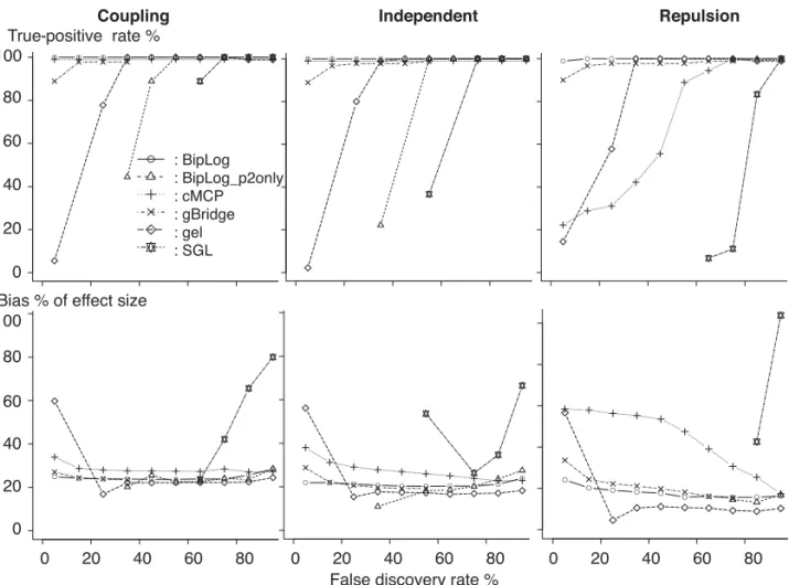
Fig. 1. Comparisons of six bilevel selection methods (SGL, gBridge, cMCP, gel), BipLog-p2only and BipLog) via simulation studies. For each of the 3 simulation scenarios with effect sizeη = 0.6, 30 traits are considered. The total number of true trait-SNP associations is 90, which includes 10 associations due to SNPs affecting only one trait (individual SNPs) and 80 associations due to SNP pairs shared across traits (shared SNPs).
three relationships between the causal SNP pairs and the two effect sizes, there are six simulation scenarios in total.
We compared BipLog with five other approaches: SGL (Simon and others,2013), gel (Breheny,
2015), gBridge, cMCP (Huangand others,2012), and BipLog with only group penaltypθ2. We used the implementation of gel, gbridge and cMCP inR/grpreg, with the default choice of 1000 tuning values for the tuning parameterλ, which were uniformly distributed on a log scale. In addition, we used the implementation of SGL inR/SGL with the default choice of 20 values of the tuning parameter. Because the R packageR/SGL can only take univariate instead of multivariate response variable, we collapseYn×q into a vector of length nq:y˜ = (y1T,. . .,yqT)T and generate a new covariate data matrix of dimension
We compare the performance of these methods across the range of tuning parameters by ROC-like curves. Specifically, instead of comparing true-positive rate (i.e., sensitivity) vs. false-positive rate (i.e., 1 - specificity) in regular ROC curves, we compare true-positive rate vs. false discovery rate (FDR). In high-dimensional settings, FDR is a more appropriate measure of accuracy than specificity. Letsbe the number of causal SNPs, and letDbe the number of discoveries, i.e., the number of nonzero regression coefficient estimates.D=TD+FD, whereTDandFDare the number of true and false discoveries. Then FDR =FD/Dand true-positive rate =TD/s. In addition, we also considered the average estimation bias of nonzero effect sizes as the average of| ˆβjk −βjk|/|βjk| ×100% for anyβjk = 0, whereβjk’s are the true effect sizes. Small bias is crucial for the success of tuning parameter selection using either BIC or cross-validation because both criterion rely on model fit, which in turn relies on unbiased estimates of effect sizes. We considered a 10% interval for the FDR from 0% to 100% and for all the models within the same FDR interval, we select the highest true-positive rate and the lowest estimation bias.
Figure1shows the median of those measurements across 100 simulations for each of the methods to be compared: BipLog, BipLog-p2only (BipLog with only group penaltypθ2), gBridge, cMCP, gel, and SGL whenη=0.6. In the “coupling” and “independent” setting, BipLog and cMCP have best performance in terms of FDR and sensitivity, and the estimates from BipLog have smaller bias than those from cMCP. In the “repulsion” setting, BipLog has much better performance than cMCP in terms of variable selection or bias. gBridge also has good performance (though slightly worse than BipLog) in all three settings. BipLog with only group penalty (BipLog_p2only) has poor performance in all the three settings. The results for η=0.3 reach similar conclusions except that cMCP shows worse performance in the independent setting and gBridge shows better performance in the repulsion setting (see Figure 1 of supplementary material available atBiostatisticsonline).
4. OMIC SIGNATURES OF CANCER DRUG SENSITIVITY
To identify the omic features associated with the cancer drugs’ sensitivity, bothGarnettand others(2012) andBarretinaand others(2012) generated omic and pharmacological data for a panel of human cancer cell lines, which represent the characteristics of various types of cancers. Garnett and others (2012) measured the mutation statuses of 64 commonly mutated cancer genes (exon sequencing), genome-wide copy number alterations (Affymetrix SNP array 6.0), and gene expression (Affymetrix HT-U133A microarray), whileBarretinaand others(2012) measured the mutation statuses of 1600 genes (targeted sequencing), genome-wide copy number alterations (Affymetrix SNP array 6.0), and gene expression (Affymetrix U133 plus 2.0 array). In the study ofGarnettand others(2012), 130 drugs were screened for drug sensitivity analysis in a range of 275–507 cell lines from a panel of 639 human tumor cell lines. In the study ofBarretinaand others(2012), 24 drugs were screened for drug sensitivity analysis for 500 cell lines on average from a panel of 947 human tumor cell lines. In both studies, the drug sensitivity was assessed by IC50, which is half-maximal inhibitory concentration. All the data used in this section were downloaded from http://www.broadinstitute.org/ccle/data/browseData and http://www.cancerrxgene.org/downloads/.
4.1 Evaluation of prediction model in the study ofGarnettand others(2012) by cross-validation
often grouped in multiple ways. There are four targeted families: chemotherapy, cytoplasmic/nonreceptor tyrosine kinase (CTK), receptor tyrosine kinase (RTK), and serine/threonine protein kinase (S/T Kinase), which include 12, 7, 10, and 30 drugs, respectively. There are 18 targeted processes (typically with less than 10 drugs per process) and 24 targeted molecules groups (typically with less than 10 drugs per molecule).
We randomly selected 65 cell lines from those with nonmissing IC50values for all 87 drugs as testing set and used the remaining cell lines as the training set. The training set was used for feature selection, and the tuning parameter was selected by the extended BIC. If a drug belonged to more than one group, we took the union of the omic features associated with that drug across the groups. To obtain the regression coefficients estimates for the union of the omic features associated with each drug, we re-estimated the regression coefficients for each drug separately using the training data (denotedβtrainˆ ) by linear regression. Thus a predictive model for each drug was obtained. Next, we used the testing data to estimate the percentage of the variance explained by the predictive model. LetSSz be the sum of squares ofz, and letytest and
Xtest be the standardized log(IC50) and omic features in the testing set. Then Prediction R-square ≡ 1− SStest
SSytest, wheretest = ytest −Xtestβtrainˆ . The possible range for prediction R-square is (−∞, 1]. To evaluate the significance of prediction R-square for a drug with k associated features, we randomly chosekfeatures from the candidate 13 847 omic features to estimate prediction R-square and repeated it for 1000 times to generate a null distribution. Then we calculated a pvalue as the percentage of the null prediction R-squares≥ the observed one. It took 8 s on average to generate thep value for each drug.
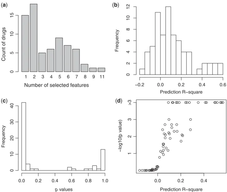
BipLog identified that 70 of the 87 drugs were associated with at least one omic feature (Figures2(a) and (b)). Forty-nine drugs had prediction R-squares greater than 0, and 17 had values greater than 20%. Forty-one of the drugs had significant prediction R-squares at the 0.05 significance level (Figure 2c), which corresponds to an estimate of FDR = 87×0.05/41≈0.1. Overall, these results suggest that the identified omic features could provide useful predictions of drug sensitivity.
4.2 Construction of prediction model using all the data fromGarnettand others(2012)
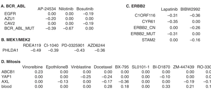
Next, we combined the training and testing sets and selected the omic features using all the available data for the 87 drugs. A few examples were shown in Figure3, and the complete results can be found in the Supplementary materials available atBiostatistics online. The abnormal gene BCR-ABL is formed by the fusion of genes BCR and ABL, and it is often observed in chronic myeloid leukemia (CML). BCR-ABL encodes a tyrosine kinase that is not regulated by cellular signals and thus causes unregulated cell proliferation, which may lead to cancer. Three drugs that target BCR-ABL protein products are included in this study (Figure3A). The sensitivity of two of these drugs is negatively correlated with the occurrence of the BCR-ABL mutation, which is expected. The negative correlation indicates that the presence of the BCR-ABL mutation is related to a reduction in log(IC50), hence an increase in the drug sensitivity.
There are two interesting new findings in this example. (i) The sensitivity of AP-24534 also increases as the expression of AZU1 increases, which is consistent with the tumor suppressor role of AZU1. (ii) The sensitivity of Bosutinib is associated with the expression of two cancer-related genes, EGFR and CAV2, instead of the BCR-ABL mutation. EGFR is a signaling protein that plays an important role in many types of cancer, and CAV2 is potentially a tumor suppressor (Leeand others,2011).
0
5
10
15
1 2 3 4 5 6 7 8 9 11
Prediction R square
Frequency
0.2 0.0 0.2 0.4 0.6
0
2
4
6
8
10
12
p values
Frequency
0.0 0.2 0.4 0.6 0.8 1.0
01
0
20
30
40
0.0 0.2 0.4
Prediction R square
log10(
p
v
alue)
1
2
3>
3
Count of drugs
Number of selected features
(a) (b)
(c) (d)
Fig. 2. Summary of the genomic feature selection results of the within-study analysis. (a) Distribution of the number of omic features selected per drug. (b) Distribution of the prediction R-squares for each drug. (c) Distribution of the pvalues of the prediction R-squares. (d) Scatter plot of the prediction R-squares and their correspondingpvalues. Since the null distribution was simulated as 1000 null samples, the smallestpvalue is 0.001.
B. MEK1/MEK2
D. Mitosis
Vinorelbine EpothiloneB Vinblastine Docetaxel BX-795 SL0101-1 BI-D1870 ZM-447439 RO-3306 ABCB1 0.23 0.00 0.00 0.00 0.00 0.00 0.00 0.00 0.00 YAP1 0.00 0.00 –0.25 –0.24 0.00 0.00 –0.10 0.00 0.00 AXL 0.00 –0.13 0.00 –0.17 –0.36 0.00 0.00 –0.19 –0.15 blood 0.00 0.00 0.00 0.28 0.18 0.00 0.33 0.21 0.15
RDEA119 CI-1040 PD-0325901 AZD6244 PHLDA1 –0.49 –0.39 –0.43 –0.36
A. BCR_ABL
AP-24534 Nilotinib Bosutinib EGFR 0.00 0.00 –0.19 AZU1 –0.20 0.00 0.00 CAV2 0.00 0.00 –0.19 BCR_ABL_MUT –0.39 –0.67 0.00
C. ERBB2
Lapatinib BIBW2992 C1ORF116 –0.31 –0.36 CYR61 –0.35 0.00 ERBB2_CN 0.00 –0.26
ERBB2_MUT –0.31 0.00 STAM2 0.00 –0.16
Fig. 3. Omic features associated with four groups of drugs that share the molecular targets BCR_ABL (A), MEK1/MEK2 (B), ERBB2 (C), or the process target Mitosis (D). For each group, the regression coefficient matrix is shown for those omic features with at least one nonzero coefficient, where a row corresponds to a genomic feature and a column corresponds to a drug. The feature X_MUT is a binary indicator showing whether gene X has mutation; ERBB2_CN is the copy number of the gene ERBB2; blood is a binary indicator showing whether the cell line is derived from a blood tumor. The remaining features are gene expressions.
Figure 3D presents the estimated coefficient matrix for nine drugs that target the Mitosis process. The features shared by several drugs include the expression of genes YAP1 and AXL and the blood-tissue indicator.YAP1 encodes “YES-associated protein 1,” which has been shown to be related to different types of cancer. AXL encodes a receptor tyrosine kinase, which is also involved with tumorigenesis. Previous studies have shown that the protein products of YAP1 and AXL may function together (Cuiand others,
2011).
4.3 Validation of the prediction model on the data fromBarretinaand others(2012)
We treated the data ofGarnettand others(2012) andBarretinaand others(2012) as the training and testing study data, respectively. Of the 24 drugs analyzed byBarretinaand others(2012), 12 were analyzed in the training study. Five of the 12 drugs had missing values in more than 325 cell lines in the training study, so they were not included in the 87 drugs in the above analysis. To address this issue, we conducted another group-wise analysis using the training data for groups involving any of these 12 drugs. Then we chose the features associated with each drug as the union of the features selected in this new analysis and those from the above analysis, whenever possible. For the 12 drugs that were analyzed using the testing data but not the training data, we fitted the prediction models using the features selected for their drug targets. For example, for the drug Topotecan, which targets the molecule TOP1, we used the features from the training study associated with the drug group that targeted TOP1 as the features associated with Topotecan.
To determine whether at least one of the selected features is associated with drug sensitivity in the testing data, we used anFtest to compare the intercept-only model and the model with all the identified omic features (Figure 4). The p values are smaller than 0.05 in most cases. The drugs PLX4720 and Lapatinib are particularly significant, withpvalues of 10−39and 10−17, respectively.
17 AAG[5]
AZD0530[3]
Irinotecan[5] Topotecan[5]
PF2341066[2]
RAF265[5]
Panobinostat[3] AEW541[1]
AZD6244[1] PD 0325901[1]
Erlotinib[2] Lapatinib[5]
1.917
ZD 6474[4] TAE684[3]
PLX4720[3]
1.239
HSP IGF1R ABL MEK1/2 EGFR TO P
MET RAF/BRAF HD AC
ALK HSP IGF1R ABL MEK1/2 EGFR
024
6
81
0
12 drugs: validated
drugs: inferred
log10(
p
v
alue)
p value:
p value:
Fig. 4. Evaluation of the predictive model in the study ofBarretinaand others(2012); the models themselves were constructed using the data ofGarnettand others(2012). The “validated drugs” are the drugs that were analyzed in both studies. The inferred drugs are the drugs that were analyzed only in the study ofBarretinaand others(2012). The x-axis shows the drug targets, and they-axis shows the−log 10(pvalues) from theFtest that compares the model with all the identified omic features to the intercept-only model using the data ofBarretinaand others(2012). The numbers in brackets are the number of features in the corresponding prediction model.
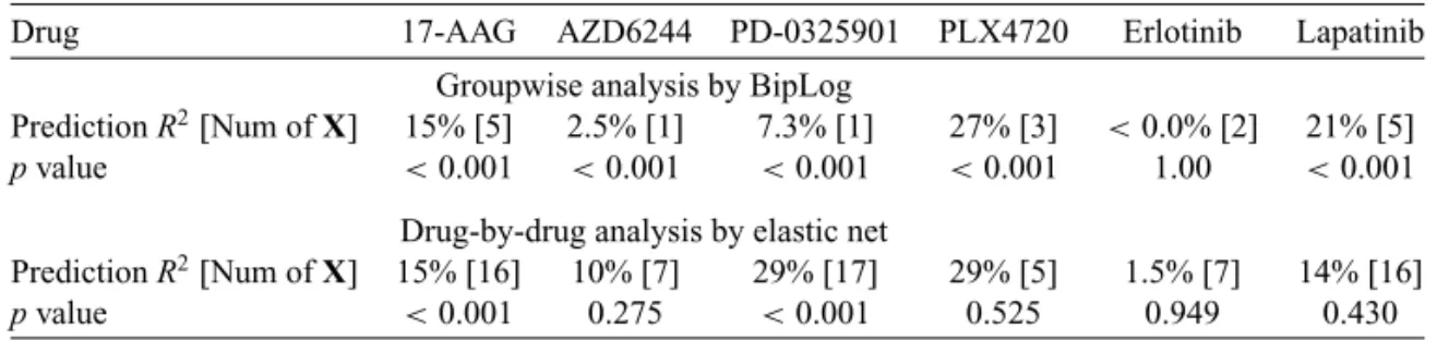
Table 1.Prediction R-squares in the study ofBarretinaand others(2012).
Drug 17-AAG AZD6244 PD-0325901 PLX4720 Erlotinib Lapatinib
Groupwise analysis by BipLog
PredictionR2[Num ofX] 15% [5] 2.5% [1] 7.3% [1] 27% [3] <0.0% [2] 21% [5]
pvalue <0.001 <0.001 <0.001 <0.001 1.00 <0.001 Drug-by-drug analysis by elastic net
PredictionR2[Num ofX] 15% [16] 10% [7] 29% [17] 29% [5] 1.5% [7] 14% [16]
pvalue <0.001 0.275 <0.001 0.525 0.949 0.430
analyzed in both the training and testing studies. Because of the disparate ranges and scales of log(IC50) in the two studies, as shown in Figure 5 of supplementary material available atBiostatisticsonline, we could not directly use the regression coefficients estimated from training study. Instead, for each drug, we randomly split the cell lines in the testing data into two groups of equal size as set 1 and set 2. We used set 1 to estimate the linear regression coefficients of the features identified by the training data. Then we used set 2 to estimate the prediction R-square. We repeated this procedure 100 times to obtain median prediction R-squares as our final estimates. Then we applied Monte Carlo simulations to evaluate the significance of the prediction R-squares, similar to our approach in Section 4.1.
5. CONCLUSION AND DISCUSSION
We have presented a new method, BipLog, for the bilevel selection of omic features related to cancer drug sensitivity. BipLog can select the covariates shared by a group of response variables as well as the covariates that are associated with one or a few of the response variables. The application of BipLog to real-data analysis reveals many interesting results. This is partly due to the strong effect size in the data. In contrast to genome-wide association studies where a genetic variant may explain only a few percentage of the variation in the trait of interest, the omic features measured in tumor tissues have a strong influence on the cancer progression and its response to drug treatment.
We have implemented our method in an R package with C code for computationally intensive part of the computation. Although using four tuning parameters does incur higher computational load, our method is computationally feasible for the problems we aim to solve. For example, in the simulation setting with
n = 200,p =562,q =30, and with a total 6000 combinations of the four tuning parameters, it takes about 30 min to finish the computation. Considering an example in our real application, it takes about 1 h to finish computation for a data set withn=462,p=13, 062, andq=8. We have also evaluated how the values of the four tuning parameters influence the performances of BipLog using the same data set used in our simulation studies withη=0.6 (See Figures 2–4 of supplementary material available atBiostatistics
online). Our results suggest the performance of our method does not change much with respect to the choice ofδ1andδ2(note thatλ1=(1+δ1)/nandλ2=(1+δ2)/n), and thus it is possible to set them as fixed values such as 3.5 or 4.0.
SUPPLEMENTARY MATERIAL
Supplementary material is available athttp://biostatistics.oxfordjournals.org.
ACKNOWLEDGEMENTS
Conflict of Interest: None declared.
FUNDING
National Institutes of Health (R03 CA167684-01 and R01 GM105785).
REFERENCES
BARRETINA, J., CAPONIGRO, G., STRANSKY, N., VENKATESAN, K., MARGOLIN, A. A., KIM, S., WILSON, C. J., LEHÁR, J., KRYUKOV, G. V., SONKIN, D.ANDothers. (2012). The cancer cell line encyclopedia enables predictive modelling of anticancer drug sensitivity.Nature483, 603–607.
BREHENY, P. (2015). The group exponential lasso for bi-level variable selection.Biometrics71, 731–740.
BREHENY, P.ANDHUANG, J. (2009). Penalized methods for bi-level variable selection.Statistics and its Interface2, 369–380.
BROMAN, K. W, WU, H., SEN, ´S.AND CHURCHILL, G. A. (2003). R/qtl: Qtl mapping in experimental crosses. Bioinformatics19, 889–890.
CAPONIGRO, G.ANDSELLERS, W. R. (2011). Advances in the preclinical testing of cancer therapeutic hypotheses. Nature Reviews Drug Discovery10, 179–187.
CHEN, T.H., SUN, W.ANDFINE, J.P. (2015). Designing penalty functions in high dimensional problems: the role of tuning parameters.Technical Report. UNC Chapel Hill.
CHEN, Y., DU, P. AND WANG, Y. (2014). Variable selection in linear models. Computational Statistics 6, 1–9.
CROFT, D., O’KELLY, G., WU, G., HAW, R., GILLESPIE, M., MATTHEWS, L., CAUDY, M., GARAPATI, P., GOPINATH, G., JASSAL, B.ANDothers. (2011). Reactome: a database of reactions, pathways and biological processes.Nucleic Acids Research39(suppl 1), D691–D697.
CUI, ZL, HAN, FF, PENG, XH, CHEN, X, LUAN, CY, HAN, RC, XU, WG, GUO, XJANDothers. (2011). YES-associated protein 1 promotes adenocarcinoma growth and metastasis through activation of the receptor tyrosine kinase axl. International Journal of Immunopathology and Pharmacology25, 989–1001.
de PALMA, M.ANDHANAHAN, D. (2012). The biology of personalized cancer medicine: facing individual complexities underlying hallmark capabilities.Molecular Oncology6, 111–127.
FAN, J.ANDLV, J. (2010). A selective overview of variable selection in high dimensional feature space.Statistica Sinica20, 101–148.
FRIEDMAN, J.H. (2012). Fast sparse regression and classification. International Journal of Forecasting 28, 722–738.
GARNETT, M.J., EDELMAN, E.J., HEIDORN, S.J., GREENMAN, C.D., DASTUR, A., LAU, K.W., GRENINGER, P., THOMPSON, I.R., LUO, X., SOARES, J.ANDothers. (2012). Systematic identification of genomic markers of drug sensitivity in cancer cells.Nature483, 570–575.
HUANG, J., BREHENY, P.ANDMA, S. (2012). A selective review of group selection in high-dimensional models. Statistical Science27, 481–499.
HUANG, J., MA, S., XIE, H.ANDZHANG, C.H. (2009). A group bridge approach for variable selection.Biometrika96, 339–355.
LEE, S., KWON, H., JEONG, K., PAK, Y.ANDothers. (2011). Regulation of cancer cell proliferation by caveolin-2 down-regulation and re-expression.International Journal of Oncology38, 1395.
MAZUMDER, RAHUL, FRIEDMAN, JEROME HAND HASTIE, TREVOR. (2011). Sparsenet: coordinate descent with nonconvex penalties.Journal of the American Statistical Association106, 1125–1138.
OBERST, MICHAELD, BEBERMAN, STACEYJ, ZHAO, LIU, YIN, JUANJ, WARD, YVONA ANDKELLY, KATHLEEN. (2008). Tdag51 is an erk signaling target that opposes erk-mediated hme16c mammary epithelial cell transformation.BMC Cancer8, 189.
SIMON, N., FRIEDMAN, J., HASTIE, T.ANDTIBSHIRANI, R. (2013). A sparse-group lasso.Journal of Computational and Graphical Statistics22, 231–245.
SUN, W., IBRAHIM, J.G.ANDZOU, F. (2010). Genomewide multiple-loci mapping in experimental crosses by iterative adaptive penalized regression.Genetics185, 349–359.
WANG, H.AND LENG, C. (2008). A note on adaptive group lasso. Computational Statistics & Data Analysis52, 5277–5286.
YUAN, M.ANDLIN, Y. (2006). Model selection and estimation in regression with grouped variables.Journal of the Royal Statistical Society: Series B (Statistical Methodology)68, 49–67.
ZHAO, P.ANDYU, B. (2006). On model selection consistency of lasso.The Journal of Machine Learning Research7, 2541–2563.
ZOU, H.ANDHASTIE, T. (2005). Regularization and variable selection via the elastic net.Journal of the Royal Statistical Society: Series B (Statistical Methodology)67, 301–320.
ZOU, H.ANDLI, R. (2008). One-step sparse estimates in nonconcave penalized likelihood models.Annals of Statistics 36, 1509–1533.