ESSAYS IN EARLY CHILDHOOD DEVELOPMENT AND PUBLIC POLICY
Jade Vanessa Marcus Jenkins
A dissertation submitted to the faculty of the University of North Carolina at Chapel Hill in partial fulfillment of the requirements for the degree of Doctor of Philosophy in the
Department of Public Policy.
Chapel Hill 2013
ii
Abstract
JADE VANESSA MARCUS JENKINS: Essays in early childhood development and public policy
(Under the direction of Gary T. Henry)
A large literature demonstrates the long-term individual and societal benefits of investing resources in children during early childhood because of the powerful influence of the environment during early life on child neurological development. Therefore, early childhood presents an unrivaled opportunity for policy intervention, and is a critical component of child and family policy.
This dissertation uses three different types of policy research to examine child well-being between birth and kindergarten. Chapter 1 is a program evaluation of a school-based outreach intervention to identify and enroll uninsured low-income children in publicly funded health insurance programs in North Carolina. Chapter 2 is a state policy evaluation examining how variations in state governance of early child care and education policy affects children’s well-being. Chapter 3 is an example of testing and applying theory from
economics to examine how parent characteristics and behaviors contribute to child cognitive development throughout early childhood. Each paper is interdisciplinary, implementing different methods for causal inference to address the unique challenges of each approach using statewide and nationally representative child data with several indicators of well-being.
iv
Dedication
Acknowledgements
The work presented in this dissertation would not exist without the help and support of many people. The length of this section is one small indication of my overwhelming and humbling sense of gratitude for the people in my professional life. First and foremost, I would like to express my abundant gratitude for my advisor, Dr. Gary Henry, for his unfailing support of my Ph.D. study and research, for the fantastic opportunities he has provided me with to learn how to conduct rigorous and truly policy-relevant research, for being an exemplar of an applied researcher, and his discerning and thoughtful feedback on all the prior drafts of this dissertation. This is in addition to the continuous support and
enthusiasm for my work he has provided over the past five years.
I am also fortunate to have a dissertation committee composed of intelligent and supportive people whose skills are complimentary to one another and who have been unsparingly generous with their time and wisdom for the past five years. I wish to
vi
I want to express my overwhelming appreciation to Dr. E. Michael Foster for his inexhaustibly honest and outstanding mentorship, training, wisdom, and criticism. He has always gone above and beyond any student’s expectations of what a mentor and professor should be and has always held me accountable to the same high standards he sets for his own professional work. My research experience and training with Dr. Foster has profoundly shaped my development as a scientist and has enabled me to successfully complete the rigorous work required of the dissertation process.
I also gratefully acknowledge Dr. Christine Durrance, with whom I was lucky enough to be advised by since the first day of the doctoral program. Dr. Durrance is not only unquestionably judicious, straightforward, and caring with her students, but she has served as a personal model of a successful, hard-working, female researcher. Her teaching, mentorship, and constant encouragement throughout my training and the contemporaneous life events have enabled me to maintain my overall well-being and have prepared me for the challenges yet to come in my career.
I want to acknowledge the Graduate School of the University of North Carolina at Chapel Hill for awarding me a Dissertation Completion Fellowship in my final year of doctoral study. The fellowship award made it possible for me to focus solely on the research presented in this dissertation. The overall quality, rigor, and comprehensiveness of the work herein are without a doubt a function of the fellowship opportunity.
I also wish to acknowledge the hard-working and devoted professional staff at the Early Learning Coalition of Alachua County, in Gainesville, Florida. It was my experience at the coalition that motivated me to pursue doctoral training in public policy in order to enact systematic changes for the well-being of young children living in poverty. I am humbled by the inexhaustible passion of these people who help children day-in and day-out, and hope that my work will one day have as great of an impact as theirs has.
viii
I would also like to recognize the institutions and data sources of the important variables for the studies in chapters one and two: Interuniversity Consortium for Political and Social Research; National Institute for Early Education Research at Rutgers University; National Center for Children in Poverty at Columbia University; National Center for Education Statistics, Institute for Education Sciences in the Department of Education; National Child Care Information and Technical Assistance Center, Administration for Children and Families in the Department of Health and Human Services; Council for State Governments; Center for American Women in Politics; Bureau of Economic Analysis in the Department of Commerce; Children's Defense Fund; Bureau of Labor Statistics; the
University of Kentucky Center for Poverty Research; NC Office of State Management and Budget; U.S. Census; NC School Nurse Council; NC Division of Health Service Regulation; and the NC State Center for Health Statistics.
Preface
Poverty and early childhood development
Poverty is a significant social problem that poses harmful and often irreversible threats to child development. Child poverty rates have been on the rise for nearly 40 years and is far more prevalent for children in the United States than for those in other
industrialized countries (Kamerman & Kahn, 1997; Smeeding, 2005). Forty-six percent of infants and toddlers live in poverty in the U.S., a rate that surpasses adults and senior citizens (Chau, Thampi, & Wight, 2010).
Thirty years of research have established that family income and other measures of socioeconomic status (SES) are associated with cognitive, behavioral and health outcomes in childhood. Poor children do worse on tests of cognitive ability, are more likely to perform poorly in their classes, have higher arrest, retention and school dropout rates, and experience more serious emotional and behavioral problems (Bradley & Corwyn, 2002 provide a comprehensive review of these studies; Brooks-Gunn & Duncan, 1997; Cunha & Heckman, 2007; Holzer, Schanzenbach, Duncan, & Ludwig, 2007; McLoyd, 1998). Both the depth of its causes and the breadth of its consequences make child poverty a concern for people across all political persuasions and academic disciplines.
x
receive welfare (Hart & Risley, 1995). The experience of poverty and distress during the first five years of life more strongly predict cognitive outcomes than poverty in middle or late childhood (G. J. Duncan, Yeung, Brooks-Gunn, & Smith, 1998), and has detrimental effects on adult earnings (G. J. Duncan, Ziol-Guest, & Kalil, 2010). This is because the child’s environment and experiences during this period lay the biological foundation for learning, health and behavior, and greatly influence their life trajectory.
For these reasons, publicly funded intervention programs target families with children ages birth to five to mitigate the consequences of poverty (Brooks-Gunn & Duncan, 1997; Gormley, Gayer, Phillips, & Dawson, 2005; Howes et al., 2008; Shonkoff & Phillips, 2000). The efficacy of early childhood intervention is supported by evidence from education, neuroscience, developmental psychology, and economics that demonstrate the importance of high-quality experiences, activities, interaction and engagement during the first five years of life on children’s cognitive and language development (Barnett, 2011; Bowman, Donovan, & Burns, 2000; Hackman & Farah, 2009; Heckman & Masterov, 2007; Magnuson &
Waldfogel, 2005; McLoyd, 1998; NICHD Early Child Care Research Network, 2005;
powerful influences—both positive and negative—on their temperament, social behavior and cognitive skills.
A developmental stage can also be considered ‘critical’ if the presence or absence of an experience results in irreversible change (Trachtenberg & Stryker, 2001). Early childhood is a critical period because the brain overproduces synapses during the first two years of life, and experience then determines which connections will persist or deteriorate from lack of use (Greenough & Black, 1992; Singer, 1995). Ergo, experiences later in life are substantially less effective in shaping many behaviors (Knudsen, Heckman, Cameron, & Shonkoff, 2006). For policies that address the consequences of child poverty, timing matters.
xii
The powerful influence of the environment during early life on child neurological development presents an unrivaled opportunity for policy action. Altogether, this research illustrates why early childhood policy is the cornerstone of a nation’s child and family policy.
Early childhood and family policy research
To be a proficient policy scholar, one must be able to understand the multiple dimensions of the particular policy field and the related research landscape. This includes the field’s constituent academic disciplines, of which there are several that are relevant to child policy. As illustrated in the previous section, the study of children and poverty is widespread. Because of this broad interest, it may not be surprising that child policy is not a cohesive or comprehensive policy field. Rather, it is a conglomeration of disparate initiatives and institutions, of assumptions and theories, of interests and investments, and of methods and causal claims. For researchers, this often renders the child development literature to be siloed by academic discipline and constrains interdisciplinary scholarship. It is therefore the task of child policy scholars to integrate these perspectives and their respective research in a practical way to understand the mechanisms of intervention and to develop innovative policy solutions.
shape family life, including the primary child and family policies. All of these perspectives play a unique role in policy analysis
Bringing together the research from diverse fields also means translating, interpreting and practicing different approaches to research design and methods. Child policy research design can be anything from a randomized experiment, a qualitative study, to a controlled laboratory that examines the genetic and biological components of human development. As a result, the analytic methods can range from bivariate, to correlational and across the full spectrum of econometric approaches.
The goals of policy research are to understand the problems of families, test policy alternatives, and assess interventions. The child policy field requires good descriptive
research of what low-income families and children are experiencing, an understanding of the emotional, cognitive and biological development of children, an interdisciplinary
understanding of the policy field and the policy intervention mechanisms, and powerful causal designs and research methods to assess the effectiveness of policies and interventions. My goal is to cover multiple dimensions of child policy research in this dissertation.
Causal inference in policy research
xiv
makes it challenging to determine whether both the treated and untreated groups would have the same potential for a given outcome; their average outcomes can either differ from: 1) the effect of the treatment, 2) differences in the individuals prior to treatment, 3) differences in the reaction to treatment, or 4) some combination of both 2 and 3. Researchers can use different design and statistical strategies to approach these challenges to causality (Shadish, Cook, & Campbell, 2002).
Structural research design features come from a theory of experimentation, whereas statistical modeling and econometric procedures stem from a non-experimental framework that uses observational data to examine economic behaviors and test theory (Shadish, et al., 2002). Research design includes the contemplating, collecting, organizing, and analyzing of data prior to outcome estimation (Rubin, 2005). In terms of design, a quasi-experimental (QE) or observational study are considered experiments that have treatments, outcomes, and units, but assign units to treatment in a way that is non-random (Cook & Campbell, 1979). A QE analysis starts by comparing the potential outcomes of the sample and carefully
considering the assignment mechanisms; essentially, researchers conceptualize the QE data as coming from a hypothetical randomized experiment (Rubin, 2008). Therefore, the randomized experiment differs only in degree from QE designs in that in the former we are confident that the causal variable of interest is independent of confounding factors, and in the latter we need to justify this with data and theory (Angrist & Pischke, 2010; Leamer, 1983).
2009). Furthermore, econometricians often criticize the randomized experimental design for its limited generalizability, ethical implications, time constraints, and ability to answer other important questions to social sciences and program evaluation (e.g. mechanisms, selection processes and economic behavior) (Heckman & Smith, 1995). Econometricians have made significant contributions to the treatment effect literature, including techniques such as instrumental variables, structural equations modeling, and propensity scores (Lee, 2005).
There is some contention in the policy evaluation literature on the experimental or design approach vs. the econometric approach (Glazerman, Levy, & Myers, 2003; Heckman & Smith, 1995). It is now well established that while both research design and statistics are critical, design is paramount (Angrist & Pischke, 2010; Rubin, 2008; Shadish & Cook, 1999; Shadish, et al., 2002). Solid statistical analysis alone cannot warrant valid causal inference; they work best after good design features are in place (Shadish, et al., 2002). Nonetheless, it is also true that policy researchers must invariably tackle non-random assignment and require econometric tools to overcome confounding. Thus, this dissertation incorporates both design and econometric techniques.
The dissertation approach
The focus of this dissertation is policy research concerning low-income families with children ages birth to five years. This dissertation is composed of three independent essays. In the following chapters, I demonstrate my command of methods for causal
inference by applying both research design and a diverse set of econometric techniques. This is complimented with strong external validity by using data that are representative of children on both the national and state levels, and robust child and family outcomes that cover
xvi
children, families, schools, counties, and states. These differences allowed me to show my ability to combine and manipulate data from numerous sources and create panel datasets for analysis. Lastly, in line with recommendations from child development and public policy scholars, this dissertation is interdisciplinary; it includes literature, theory, and methods from economics, developmental psychology, political science, public health, education,
neuroscience, and sociology.
I have designed these essays so that each paper is an example of a different type of policy research: program evaluation, state policy evaluation, and testing and advancing theory. Each paper shows a particular kind of method, depth, and theoretical motivation, and the analyses address the unique challenges of the research approach. In combination, I believe that all of these components create the foundation for a strong dissertation that meets the requirements of the Doctor of Philosophy degree in Public Policy. In the following chapters I present each of the above papers in turn as independent, stand-alone studies.
Chapter 1 is a program evaluation of a school-based outreach intervention to enroll low-income children in publicly funded health insurance programs in North Carolina. This paper shows my ability to use program evaluation methods with a strong causal design to address selection bias, the primary threat to causality when examining program take-up. This paper also uses mixed-methods and cuts across public health and education. The findings may help to expand our understanding of preventive health care use among low-income families and the role of schools in public health research.
understanding of the endogeneity of policy adoption and address threats to causality with a number of econometric tools. I also show my ability to integrate research from policy management and administration, political science, and early childhood education. This study provides empirical bases for how the governance of state policy influences policy outcomes. In chapter 3, I use current research in neuroscience and developmental psychology in the context of economic theory to examine the allocation of household resources,
including family characteristics and behaviors, during early childhood. I apply the theoretical research to policy by conceptualizing family factors as intervention mechanisms to mitigate the effects of poverty on child development.
TABLE OF CONTENTS CHAPTER 1.!THE EFFECTS OF A SCHOOL-BASED PUBLIC HEALTH INSURANCE OUTREACH PROGRAM ON HEALTH
CARE USE IN KINDERGARTEN-AGED CHILDREN ... 1!
INTRODUCTION ... 1!
BACKGROUND AND LITERATURE ... 4!
Benefits and costs of health insurance coverage for children ... 4!
Medicaid and the State Children’s Health Insurance Program ... 6!
CHIPRA outreach and the NC Healthy and Ready to Learn initiative ... 10!
DATA ... 14!
Kindergarten Health Assessment (KHA) forms ... 14!
Medicaid and SCHIP administrative dataset ... 15!
Focus Groups and Key Informant Interviews ... 18!
METHODS ... 19!
Descriptive Analysis ... 19!
Regression Discontinuity Design ... 19!
Model specifications ... 24!
Focus group and interview design ... 27!
RESULTS ... 29!
Descriptive Analysis ... 29!
Regression Discontinuity ... 31!
Difference-in-Differences ... 33!
Summary ... 35!
Focus Group and Interview Data Analysis ... 36!
DISCUSSION ... 39!
CHAPTER 2.!THE EFFECT OF STATE POLICY GOVERNANCE ON EARLY CHILDHOOD OUTCOMES ... 55!
INTRODUCTION ... 55!
BACKGROUND ... 58!
Child policy at the state level ... 60!
Governance of ECCE policy ... 63!
THEORETICAL RATIONALES FOR POLICY GOVERNANCE ... 70!
Causality and state policy research ... 76!
DATA ... 79!
Child and family-level ... 79!
State-level ... 80!
METHODS ... 81!
Econometric approaches to address state policy endogeneity ... 81!
Instrumental Variables Estimation ... 84!
Model specification and estimation ... 88!
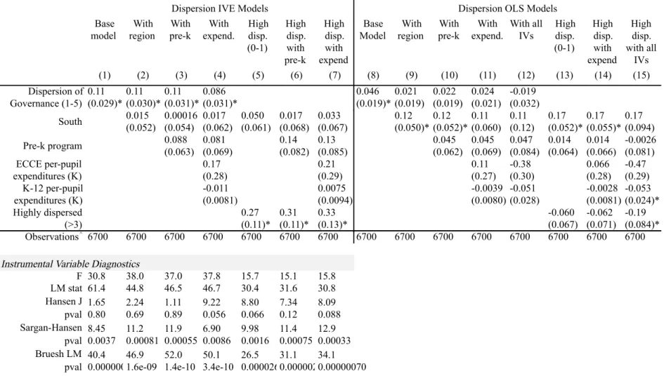
RESULTS ... 91!
Instrumental Variable Diagnostics ... 91!
Dispersion of governance ... 93!
Expenditures ... 97!
DISCUSSION ... 98!
Future research ... 105!
CHAPTER 3.!PARENTING SKILLS AND EARLY CHILDHOOD DEVELOPMENT: PRODUCTION FUNCTION ESTIMATES FROM
LONGITUDINAL DATA ... 115!
INTRODUCTION ... 115!
THEORETICAL FRAMEWORK ... 119!
a. The household production model ... 119!
b. Specification of the child development production function ... 121!
DATA ... 123!
a. Child ability measures ... 124!
b. Inputs and covariates ... 125!
RESULTS ... 129!
a. Alternative specifications of the CDPF ... 129!
b. Parenting Skills ... 133!
c. Input Demand Functions ... 136!
d. Endogeneity ... 137!
DISCUSSION ... 143!
APPENDICES ... 157
LIST OF TABLES
TABLE 1.1:COUNTY-LEVEL VARIABLES, DESCRIPTIVE STATISTICS AND DATA
SOURCES FOR 2010 ... 45!
TABLE 1.2:SAMPLE PROPORTIONS FOR SELECTED HEALTH CHARACTERISTICS
FROM THE KINDERGARTEN HEALTH ASSESSMENT (KHA)FORM ... 46!
TABLE 1.3:ENROLLMENT RATES AND WELL-CHILD EXAM RATES BY YEAR AND
BY TREATMENT STATUS ... 47!
TABLE 1.4:KINDERGARTEN HEALTH ASSESSMENT (KHA) SAMPLE AND
STATEWIDE KHA SAMPLE OF THE PERCENT MISSING ON KHA
PARENT REPORT ITEMS ... 48!
TABLE 1.5:MODEL RESULTS FOR THE EFFECT OF HRL ON MEDICAID AND
SCHIPENROLLMENT RATES FOR KINDERGARTEN-AGED CHILDREN ... 49!
TABLE 1.6:MODEL RESULTS FOR THE EFFECT OF HRL ON MEDICAID AND
SCHIP WELL-CHILD EXAM RATES FOR KINDERGARTEN-AGED
CHILDREN ... 50!
TABLE 2.1:VARIABLE NAMES, DESCRIPTIVE STATISTICS, AND DATA SOURCE
BY VARIABLE TYPE ... 107!
TABLE 2.2:INSTRUMENTAL VARIABLES ESTIMATION AND OLS RESULTS FOR THE EFFECT OF POLICY GOVERNANCE ON KINDERGARTEN
READING SKILLS ... 109!
TABLE 2.3:INSTRUMENTAL VARIABLES ESTIMATION AND OLS RESULTS FOR THE EFFECT OF POLICY DISPERSION ON KINDERGARTEN MATH
SKILLS ... 110!
TABLE 2.4:INSTRUMENTAL VARIABLES ESTIMATION AND OLS RESULTS FOR THE EFFECT OF POLICY DISPERSION ON KINDERGARTEN FINE
MOTOR SKILLS ... 111!
TABLE 2.5:INSTRUMENTAL VARIABLES ESTIMATION AND OLS RESULTS FOR THE EFFECTS OF POLICY DISPERSION ON AGE-FOUR (PRESCHOOL)
TABLE 2.6: INSTRUMENTAL VARIABLES ESTIMATION RESULTS FOR THE EFFECT OF POLICY EXPENDITURES ON KINDERGARTEN READING, MATH,
FINE MOTOR, AND AGE-FOUR READING SKILLS ... 113!
TABLE 3.1: DESCRIPTIVE STATISTICS BY MEASUREMENT WAVE (WEIGHTED) ... 147!
TABLE 3.2:ESTIMATES OF THE CDPF FOR READING IN KINDERGARTEN ... 148!
TABLE 3.3:ESTIMATES OF THE CDPF FOR READING IN PRESCHOOL ... 149!
TABLE 3.4:ESTIMATION OF INPUT DEMANDS FOR READING AT PRESCHOOL,2
YEARS, AND 9 MONTHS OF AGE ... 150!
TABLE 3.5:PANEL DATA MODELS FOR READING IN PRESCHOOL ... 151!
TABLE 3.6:FREQUENCIES OF PARENT READING INVESTMENT PATTERNS OVER
THE FOUR WAVES OF DATA ... 152!
TABLE 3.7:FAMILY AND CHILD CHARACTERISTICS BY READING PATTERN
LIST OF FIGURES
FIGURE 1.1:MAP OF N.C.COUNTIES IN THE HEALTH AND READY TO LEARN
INITIATIVE TREATMENT ... 51!
FIGURE 1.2:KINDERGARTEN HEALTH ASSESSMENT (KHA)FORM WITH
HEALTH INSURANCE ITEM IDENTIFIED ... 52!
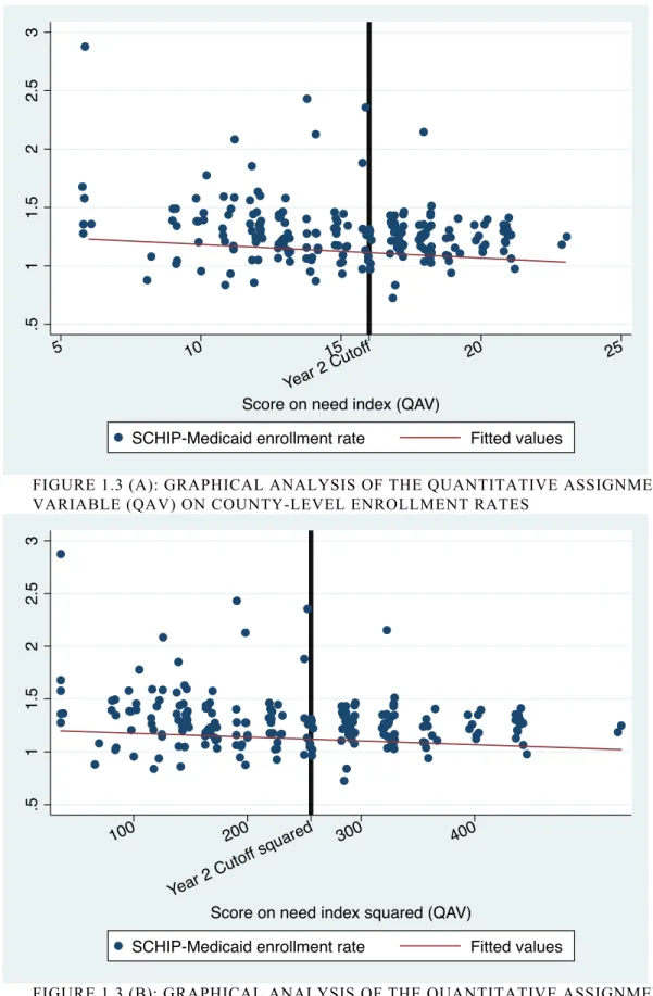
FIGURE 1.3(A): GRAPHICAL ANALYSIS OF THE QUANTITATIVE ASSIGNMENT
VARIABLE (QAV) ON COUNTY-LEVEL ENROLLMENT RATES ... 53!
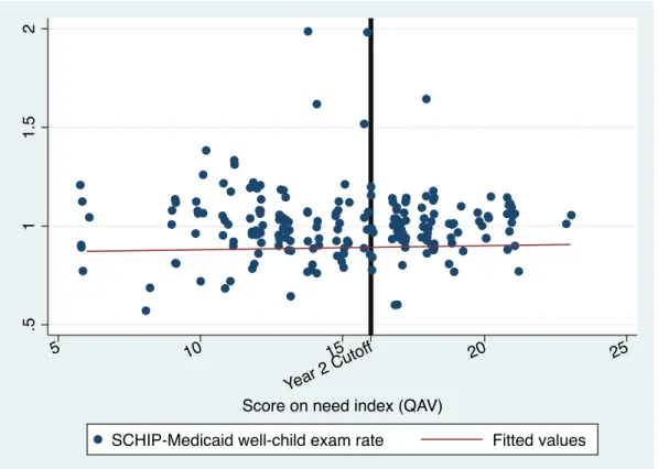
FIGURE 1.3(B):GRAPHICAL ANALYSIS OF THE QUANTITATIVE ASSIGNMENT VARIABLE (QAV) SQUARED ON COUNTY-LEVEL ENROLLMENT
RATES ... 53!
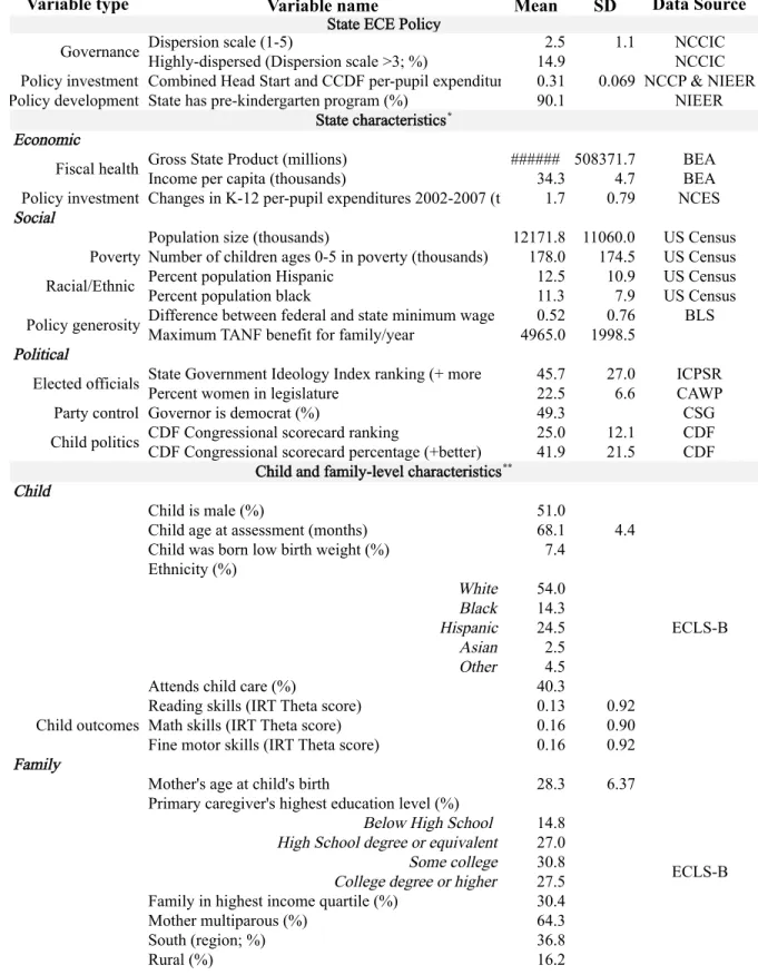
FIGURE 1.4(A): GRAPHICAL ANALYSIS OF THE QUANTITATIVE ASSIGNMENT VARIABLE (QAV) ON COUNTY-LEVEL WELL-CHILD EXAM
RATES ... 54!
FIGURE 1.4(B): GRAPHICAL ANALYSIS OF THE QUANTITATIVE ASSIGNMENT VARIABLE (QAV) SQUARED ON COUNTY-LEVEL WELL-CHILD
EXAM RATES ... 54!
FIGURE 2.1:NUMBER OF FEDERAL PROGRAMS THAT PROVIDE OR SUPPORT EDUCATION AND CARE FOR CHILDREN UNDER AGE 5, BY
DEPARTMENT OR AGENCY ... 114!
FIGURE 3.1:READING ABILITY ACROSS 4 MEASUREMENT WAVES BY PARENT
-CHILD READING PATTERNS ... 154!
FIGURE 3.2:AGE OF PARENT’S READING INITIATION BY CHILD BIRTHWEIGHT
(ENDOWMENT) ... 155!
FIGURE 3.3: READING ABILITY AT EACH WAVE BY AGE OF PARENT’S READING
LIST OF ABBREVIATIONS
ECCE Early child care and education
ECLS-B Early Childhood Longitudinal Study – Birth Cohort CCDF Child care and Development Fund
CDF Children’s Defense Fund
CDPF Child development production function
CHIPRA Children’s Health Insurance Program Reauthorization Act CMS Centers for Medicare and Medicaid Services
DID Difference-in-Differences DMA Division of Medical Assistance FPL Federal poverty level
HHS Department of Health and Human Services HRL Healthy and Ready to Learn
IDEA Individuals with Disabilities Education Act IRT Item response theory
IVE Instrumental variables Estimation KFF Kaiser Family Foundation
KHA Kindergarten health assessment NC North Carolina
NCATS Nursing Child Assessment Teaching Scale NPM New Public Management
OLS Ordinary least squares
PCG Primary caregiver
PRWORA Personal Responsibility and Work Opportunities Reconciliation Act QAV Quantitative assignment variable
RD Regression discontinuity
SCHIP State Children’s Health Insurance Program SD Standard deviation
TANF Temporary Assistance to Needy Families TBT Two-bags task
CHAPTER 1. THE EFFECTS OF A SCHOOL-BASED PUBLIC HEALTH INSURANCE OUTREACH PROGRAM ON HEALTH CARE USE IN KINDERGARTEN-AGED CHILDREN
Introduction
Public health insurance is a critical component of child and family policy. Presently, over eight million children in the U.S. are uninsured while health care costs continue to rise and families struggle to find affordable care (Kaiser Family Foundation (KFF) 2011). Medicaid and the State Children’s Health Insurance Program (SCHIP) are the largest government interventions in child health insurance coverage, and account for a significant share of health care spending overall. Together, these two programs have successfully increased rates of child insurance, particularly since the enactment of SCHIP in 1997 and the subsequent expansion income eligibility to cover more low-income working families though the CHIP Reauthorization Act (CHIPRA) in 2009. However, the current uninsured rate among children from birth to age 18 remains stagnant—around seven percent—as policymakers struggle to figure out how to successfully enroll the millions of eligible yet uninsured children (R. A. Cohen & Martinez, 2012).
significant costs for both families and society at-large. Yet it is unclear that providing health insurance to uninsured children affects whether parents actually access preventive care for their children.
If there is a relationship between insurance coverage and receipt of health care, the 8.3 million uninsured children in the U.S. are an important policy concern (Kaiser Family Foundation, 2011). When children do not receive routine preventive care, they have worse health outcomes overall including lower rates of vaccination, reduced likelihood of
identifying problems that require early interventions, and more inappropriate use of
emergency department services (Kenney, Marton, Klein, Pelletier, & Talbert, 2011). This not only affects their ability to focus and attend school, it also affects their educational and labor market outcomes in the future (Currie, 2009; Thies, 1999). The negative externalities of poor child health are also costly for society because uninsured children have more expensive health care, of which their families can only afford to pay a portion of; the rest passed on to taxpayers (North Carolina Institute of Medicine (NCIOM), 2009). This is in addition to the public health costs from illness due to missed vaccinations (Zhou et al., 2005).
2010 and 2011 school years. Sixteen counties in NC were selected for the intervention based on an index of economic need. School personnel in treatment counties were trained on program requirements and how to identify potentially eligible children using the
Kindergarten Health Assessment form (KHA). The KHA is a required document for all children entering kindergarten that contains important health information including insurance status and other key health indicators that are valuable to educational and medical
professionals, as well as policymakers.
The goals of this study are threefold. We assess: 1) whether the HRL intervention was effective at increasing Medicaid and SCHIP enrollment rates for kindergarten-aged children; 2) whether HRL increased preventive care use in SCHIP and Medicaid for
Background and literature
Benefits and costs of health insurance coverage for children
The motivation behind public health insurance for children is to improve child well-being by increasing access to and use of preventive care, providing emergency coverage, and decreasing the costs of sickness without coverage (Kenney, et al., 2011; C. D. Perry & Kenney, 2007). Uninsured children have less access to health care services, more serious health problems, are more likely to forgo or not receive essential health care, and also use more expensive medical services than children in public or private insurance programs (Arroyo, Ewen Wang, Saynina, Bhattacharya, & Wise, 2012; Byck, 2000; Mannix, Chiang, & Stack, 2012; Newacheck, Hughes, & Stoddard, 1996; Newacheck, Stoddard, Hughes, & Pearl, 1998; Ziller, Lenardson, & Coburn, 2012). In many ways, lack of coverage presents threats to children’s development, family well-being, community and school health, and to society at-large.
school attendance, concentration and participation, but poor health is also bad for children’s future educational, health, and labor market outcomes (Case, et al., 2005; Currie, 2009; Thies, 1999).
High rates of uninsured children create other significant costs for society. The uninsured forego care and exacerbate certain health conditions putting them in emergency care (Arroyo, et al., 2012; Hadley, 2007; Wisk & Witt, 2012). Indeed, one-quarter (23%) of uninsured children have delayed or postponed care because of cost relative to 3% of insured children (Kaiser Family Foundation, 2011). They also pay for one-third of their care out of pocket, with the remainder of the costs covered by higher taxes and insurance premiums (NCIOM, 2009). In North Carolina, individuals pay an average of $438 more a year, with families paying an extra $1,130 per year on health insurance premiums to help cover the costs of uncompensated care for the uninsured (Stoll, 2005).
spent on the routine childhood immunization schedule saves more than $5 in direct costs and approximately $11 in additional costs to society due to contagion (Zhou, et al., 2005).
Routine visits are also important for child and family well-being in the long term. During these visits, physicians assess biomedical health, development, family functioning, and identify potential problems (Dinkevich & Ozuah, 2002). This is critical for the timely detection of health, developmental, and behavioral problems that may require early
intervention. A physician’s early diagnosis has the potential to reduce mortality, morbidity, and disability and enable children to lead healthier and more productive lives (Halfon & Olson, 2004; Shonkoff & Phillips, 2000). Well-child visits also give physicians the opportunity to provide anticipatory guidance, which is practical and developmentally appropriate information about children’s health such as injury prevention, nutrition, and immunizations (Dinkevich & Ozuah, 2002; Hagan, et al., 2008).
There is a clear policy rationale for public health insurance based on the benefits for children, families, and the public. Still, the connection between the policy lever of public health insurance and child well-being is no small step. The implementation of Medicaid and SCHIP involves policy actors at the federal, state, and local levels to successfully translate the funding and administration of these policies to the recruitment and enrollment of eligible children before public insurance can increase the use of preventive care.
Medicaid and the State Children’s Health Insurance Program
18 whose families are at 100% of the FPL or below (HHS-CMS, 2009). Federal investment increased in 1997 when Congress authorized almost $40 billion for the State Children’s Health Insurance Program (SCHIP), the largest single expansion of health insurance coverage for children in over 30 years (HHS-CMS, 2009). Within federal guidelines, each state determines the design of its CHIP program including eligibility parameters, benefit packages, payment levels for coverage, and administrative procedures (HHS-CMS, 2009). The federal government matches state funding for both programs but unlike Medicaid, states receive a capped allotment of CHIP funds.
From 1998 to 2007, SCHIP allowed states to provide health insurance to children from low-income, working families earning between 100 to 200 percent of the FPL who were not covered by Medicaid (General Accounting Office, 2000b). By 2003, the uninsured rate among children dropped below 12.5, the lowest since 1977, and the number of eligible but uninsured children fell 25% between 2001 and 2005 (Hudson & Selden, 2007). Rates of coverage continued to increase through 2005, and some studies indicate that the expansion in eligibility reduced the uninsured rate among children (Hudson & Selden, 2007). The
increased outreach efforts under SCHIP are also associated with the spikes in enrollment during this period (Duderstadt, Hughes, Soobader, & Newacheck, 2006).
2009; Kaiser Family Foundation, 2011). A recent meta-analysis of Medicaid and CHIP expansions shows clear gains in public health insurance coverage and declines in uninsured among children (Howell & Kenney, 2012).
Today, Medicaid and SCHIP together cover over half (59%) of low-income children, bringing the national rate of children insured to over ninety percent (Kaiser Family
Foundation, 2011). This coverage is especially important in the face of increased unemployment because these programs offset most of the decline in families’ employer-sponsored insurance (Dorn, Bowen, Holahan, & Williams, 2008; Ross & Marks, 2009). Yet the question still remains as to whether increasing enrollment and opening up eligibility for public insurance programs will increase preventive care use for children.
The effects of Medicaid and SCHIP on child health
Before the enactment of SCHIP, studies from Pennsylvania (Lave et al., 1998), New York (Szilagyi et al., 2000), and Florida (Shenkman et al., 1997) found that children who were enrolled in a state insurance program for low-income children had significant
improvement in health care access, utilization, and quality of care (Szilagyi et al., 2004). One study showed that children enrolled in Medicaid or SCHIP were more likely than full-year-uninsured and part-year-full-year-uninsured children to have had a preventive visit at a doctor’s office or clinic in the past 12 months (C. D. Perry & Kenney, 2007). Children who were uninsured for part-year were more likely to have had a preventive visit than children who were
access to care for enrollees as well (Slifkin, Freeman, & Silberman, 2002). Analyses using more nationally representative data indicate that children with continuous public coverage had significantly better access and utilization of health care when compared with eligible but uninsured children, and had equivalent or better access and utilization compared to children with private coverage (Duderstadt, et al., 2006; Howell & Kenney, 2012; Szilagyi, et al., 2004).
Still, there is significant variation across states with respect to SCHIP enrollment and retention policies (Ross & Marks, 2009) and participation rates (Kenney, Lynch, Cook, & Phong, 2010), and variation in national estimates of Medicaid and SCHIP children who receive a well-child visit (Kenney, et al., 2011). Causal analyses are critical to substantiate or refute the correlational evidence because selection bias and confounding by unobserved health factors are central issues in studies on public health insurance (Hadley, 2003). The strongest evidence to date on the effectiveness of public health insurance programs comes from the recent evaluation of the Oregon Health Insurance Experiment. Adults were randomized through a lottery system into Medicaid and after one year, the treatment group had substantively and statistically significantly higher health care utilization (including primary and preventive care as well as hospitalizations), lower out-of-pocket medical expenditures and medical debt and better self-reported physical and mental health than the control group (Finkelstein et al., 2011).
between health insurance and health care access, especially when evaluated using a strong research design. In the following sections, we describe the details of one such initiative and the research evaluation approach we use to study the relationship between outreach,
enrollment, and preventive care use with respect to public health insurance programs for children.
CHIPRA outreach and the NC Healthy and Ready to Learn initiative
Not long after the initial launch of SCHIP, it became clear that different outreach strategies were required to reach the various sub-populations of eligible children (I. Hill, 2002). CHIPRA included outreach and enrollment grants and bonus payments to states for adopting identified enrollment and retention strategies or increasing enrollment beyond expected targets (Horner, et al., 2009). By April of 2010, the federal government had awarded $50 million in outreach grants. These grants are important for enrolling uninsured children because initial evidence from national SCHIP evaluations estimate that one-third of eligible but unenrolled children have not enrolled because of knowledge gaps (Dubay, Kenney, & Haley, 2002). Studies suggest that Medicaid or SCHIP-eligible families could benefit from targeted engagement strategies linking them with consistent and appropriate sources of pediatric health care (Cullen, Matejkowski, Marcus, & Solomon, 2010), and most states promoted both programs jointly to increase enrollment (M. J. Perry, 2003). All of these factors led to the development of the outreach initiative evaluated in the present study.
programs insured nearly 800,000 children (Task Force for a Healthier Carolina, 2007). CHIPRA increased North Carolina’s 2009 SCHIP allotments over the previous law by 81 percent (Peterson, 2009). However, in 2009, three out of every five uninsured NC children were eligible for, but were not enrolled in one of the two programs (NCIOM, 2009). This disparity stemmed from both insufficient outreach efforts and a need to simplify the enrollment and renewal processes (Task Force for a Healthier Carolina, 2007).
In October 2009, North Carolina received a $678,210 CHIPRA Cycle I Outreach and Enrollment grant for the initiative Healthy and Ready to Learn (HRL). In line with the joint policy initiative by the National Association of the State Boards of Education and the Centers for Disease Control, HRL focuses on schools as a source of health information and a context to develop fit and healthy children who are ‘ready to learn’ (2000). School-linked initiatives are important because children enter schools with myriad social, health, and developmental issues (Konrad, 1996). The HRL intervention was a targeted, school-based SCHIP and Medicaid outreach and enrollment initiative for identifying and enrolling eligible and
uninsured children entering kindergarten in NC’s 16 highest-need counties, led by the North Carolina Pediatric Society Foundation (NCPSF). The HRL goals were to: 1) increase
enrollment of eligible but uninsured kindergarten-aged children in NC high-need counties; 2) improve efforts for outreach and enrollment by identifying uninsured children using the Kindergarten Health Assessment (KHA) information; 3) establish strong relationships with school nurses and School Health Advisory Councils; and 4) identify successful strategies for school-based outreach programs to extend outreach and enrollment efforts across the state.
Inthe first year (2009-10), 16 counties were selected as intervention sites based on an economic need index that included 278 elementary schools in 22 Local Education Agencies (LEA) or districts. The University of North Carolina Sheps Center for Health Services Research developed the quantitative need index used to determine the counties who received the intervention. This index incorporated county-level data on two economics-related measures (percent of children ages birth to 18 in poverty and the unemployment rate for April/May 2009) as well as the number of children who could potentially be reached by the intervention (number of children aged six to eight). The index measure values by county are displayed in Appendix A.
Each LEA in the treated counties received $3000 to use for program purposes at their own discretion. In year two, the intervention was extended to an additional 32 counties who were also selected based on the ranking of their index score. The second group had greater geographic spread and fewer HRL staff members per county (1:8 in the pilot group, 1:16 in the second group). Figure 1 shows a map of the intervention counties by year.
The primary component of the initiative was a series of regional trainings in the selected pilot school districts for local school-based personnel, primarily school nurses and administrative staff. Under the NC Health Assessment Law (G. S. 130A-440), every child entering kindergarten in public schools must receive a health assessment by a medical provider no more than 12 months prior to school entry. ). The KHA is a required document for all children entering kindergarten that contains important health assessment data
entering their school. The HRL initiative highlighted the section of the KHA form where parents indicate whether the child has Medicaid, private insurance/HMO, or no insurance, outlined in red in Figure 2. Nurses and staff could then identify uninsured children and refer their families to local partners for potential Medicaid/SCHIP enrollment.
HRL staff conducted a similar web-based training with physicians, nurses and other health care providers in pilot counties to encourage providers to talk with families about insurance coverage during the well-child visit for the purposes of filling out the KHA form. HRL also involved continuous community-based outreach throughout the study period. This included attending community events, providing outreach materials in various languages, assisting schools in their outreach programs and troubleshooting, and contacting local organizations and community leaders to help inform families about SCHIP and Medicaid.
An additional goal of the HRL program was to increase the completion rate of the parent report items on the top of the KHA form (the grey box at the top of Figure 1.2). Because the health care provider fills out most of the form, there is historically low completion of the parent section. However full completion was essential to the eligibility identification strategy of HRL—using the health insurance status item on the KHA (marked in red in Figure 1.2). A statewide probability sample of KHA forms collected by the NC Department of Health and Human Services, School Health Division in 2008 confirmed the high rate of missingness on these forms (North Carolina Department of Health and Human Services & Devision, 2009). Therefore, teachers and other school administrative staff were instructed to check the parent report section of the KHA form before accepting it from the parent or child, and returning it to them if incomplete.
This study is a comprehensive evaluation of NC’s HRL initiative. We assess whether the HRL intervention was effective at increasing Medicaid and SCHIP enrollment, and assess whether HRL increased preventive care use (i.e. well-child exams) in SCHIP and Medicaid for the target population in treated counties. Our primary treatment effect identification strategy is a Regression Discontinuity design (RD) estimator, taking advantage of the quantitative index measure used to assign counties to HRL treatment. We use statewide administrative data from the NC Department of Medical Assistance (DMA) in conjunction with other county-level data in our analyses, and also test for the robustness of our RD estimator using multiple model specifications and estimation strategies.
In addition to the quantitative analyses that test for the overall effect of HRL, we also wanted to assess best practices in school-based and community outreach efforts and to identify any other hidden treatments occurring in HRL counties. Therefore we conducted focus groups and key informant interviews with school nurses in the 16 HRL pilot counties. In combination, this study adds to the public health intervention and evaluation literature concerned with the role of schools in child health and the extent to which access to public health insurance changes the health behaviors of families with young children.
Data
Kindergarten Health Assessment (KHA) forms
the 16 pilot counties were required to photocopy the front-side of the KHA form (Figure 2) for the first intervention year, and to send these copies to the evaluation team. Trained undergraduate research assistants manually coded the forms into an electronic database using Qualtrics Survey Software. The resulting dataset includes the child’s name and birthdate, health insurance status, and more than 60 coded child health items. The full sample for the KHA data is 15,397 kindergarten children in 12 of the 16 HRL pilot counties.1 Sample proportions for a selected set of items from the KHA are listed in Table 1.2.
Medicaid and SCHIP administrative dataset
We calculated county-level health insurance enrollment and preventive care usage from the Medicaid and SCHIP claim data for all counties in NC. These are comprehensive administrative data collected by the DMA and include all claims made by children living in NC who were kindergarten aged in the 2007-08 through 2010-11 school years. The data contain three cohorts of kindergarteners who were enrolled in Medicaid or SCHIP (one year prior to intervention and two intervention years). The raw data were in long format where each observation represents a unique claim for a child, with approximately nine million observations in total. In the first treatment year, there were approximately 134,000 kindergarten-aged children enrolled in Medicaid or SCHIP. Variables include name, birthdate, county of residence, claim type and the total amount paid for each claim. Claim types include dental, drug and well-child health screenings. We therefore use the presence of a well-child exam claim as our measure of preventive care use, and refer to it as such.
1
Due to funding and time constraints, KHAs were coded only for a subsample of the 16 pilot counties.
2
We identified children in the DMA file as a member of the 2008-09, 2009-10, or 2010-11 kindergarten cohorts if they were five years of age on or before July 1st of one of the above academic years, including only one observation per child to represent enrollment.2 Similarly, we identified the number of well-child exam claims using the claim type variable for Health check/screening, including only one observation per child. These data were then aggregated to the county-level by year. Each observation in the analysis dataset then represented a county’s enrollment rate, well-child claim rate, HRL status and values of the control variables in a given year, and thus includes 300 observations (100 counties * 3 years).
Note that this sample represents every county in NC, and the KHA sample described above is a subset of the HRL pilot counties. Therefore the latter represents the NC counties with the highest economic need (as measured by the index) and are not representative of all counties in NC.
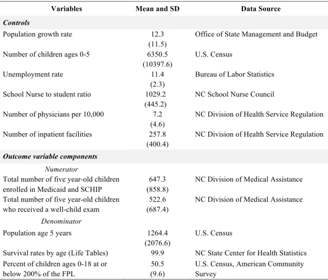
Control and outcome variables
County-level covariates were extracted from numerous data sources to use as controls in the outcome analysis and are listed in Table 1.1. Parts of our dependent variables were constructed using the DMA administrative claims data as described above. These data allowed us to determine the total number of children enrolled and number of children who received a well-child exam in each county, but they do not indicate the proportion of income- and age-eligible children by county that these numbers represent. Therefore, we needed to conduct some additional calculations incorporating other data in order to develop enrollment and well-child exam rates to use as dependent variables. Principally, this involved
2
estimating an appropriate denominator—the total number of children who are income- and age-eligible for Medicaid and SCHIP by county.
The study target population was kindergarten-aged children, so we defined the age-eligible population as the total number of five-year-old children living in the county from the 2010 Census. We adjusted this number for survival with demographic calculations3 using Sprague multipliers based on county- and state-level statistics. We then adjusted this number for poverty using the 2011 Census American Community Survey (ACS) estimates of the number of children ages 0-18 living at or below 200% of the FPL in each county (i.e. the SCHIP/Medicaid eligibility limit) to determine the proportion of children who were income-eligible (U.S. Census Bureau, 2012). These estimates became our denominators for both the enrollment and well-child exam outcome measures so that they respectively represent the proportion of age- and income-eligible children enrolled, and those who received a well-child exam during the intervention period. The variables involved in this calculation, mean values, and data sources are listed in Table 1.1.
The mean values of these estimates for enrollment and well-child exam rates are displayed by year in Table 1.3. Note that a key weakness of our dependent variable
calculation is that many of the calculations are above one, which is seemingly unreasonable for measures of rates. This is because the 2011 ACS numbers that we used to represent the proportion of children living in poverty are estimated based on the 2010 Census and therefore are not 'true' population parameters. We suspect that the 2011 ACS estimates for county-level poverty underestimate the true number of children living below 200% FPL and are thereby eligible for SCHIP or Medicaid, in part because the economic recession likely caused
3 Dr. Suchindran, demographer and Professor of Biostatistics at UNC, provided consultation to generate these
drastic changes in families’ poverty status during this time. Because of this, it appears as though there are more income- and age-eligible children enrolled than there are income- and age-eligible children in the county (i.e. number of kids enrolled>number five year olds who are below 200% FPL). As a result, our enrollment and well-child exam rates are
significantly above 100 percent because the estimated denominator we use in our calculations is in all likelihood lower than the ‘true’ denominator. Therefore, our calculations provide a relative measure of differences in rates between the groups, but do not represent true or absolute rates.
Focus Groups and Key Informant Interviews
We conducted four focus groups and five key informant interviews across the HRL regions. We collected these data to: assess best practices in school-based and community outreach efforts, document the specific activities involved in the implementation of the HRL intervention, assess the extent to which participants felt that the HRL intervention activities helped to accomplish the stated goals of HRL, and to identify any other hidden treatments that may threaten the validity of the effect estimates. Focus group participants and
focus group sessions. The UNC-Institutional Review Board approved this research in April 2011 (IRB #11-0564).
Methods
Descriptive Analysis
We calculate 2010 mean and standard deviation values for each county covariate, and the variables used to compose our outcomes, and sample proportions for a selected number of child health characteristics from the 2010 KHA dataset. We present our estimated dependent variables by year and HRL treatment status. We also compare the rates of
missingness for the parent report items on the KHA form between the HRL KHA sample (2010) and the statewide probability sample data collected in 2008 to detect whether the HRL efforts improved item completion.
Regression Discontinuity Design
Selection bias is the primary challenge to detecting causal treatment effects when the treatment outcome is program participation or enrollment. In the present study, both
treatment and outcomes are at the county-level. Selection bias is possible if unobserved county-level characteristics influence the county’s willingness to implement a health insurance outreach program like HRL. For example, counties with worse child outcomes may be more likely to participate, or counties that are not as efficacious at enrolling children in public health insurance may be less likely to participate. The former would deflate the effect of the HRL program, while the latter would inflate the effect.
method will exploit the fact that HRL treatment counties were selected using an economic need index. The primary condition for unbiased causal effects with an RD analysis is the use of a quantitative assignment variable (QAV) and a designated cutoff score or value to
determine treatment status (Imbens & Lemieux, 2008; Shadish, et al., 2002). This means that with an RD the probability of receiving treatment must change discontinuously at the cutoff as a function of the QAV (Van Der Klaauw, 2008). This is the key advantage of the RD; the researcher can capitalize on completely known and perfectly measured selection, and thus perfectly model selection by conditioning on the value of the QAV in the outcome analyses (Shadish, et al., 2002). If the assignment variable is a deterministic function of assignment to treatment, this is considered a ‘sharp discontinuity’ (Van Der Klaauw, 2008). In the current study, the index of economic need used to select HRL counties is a perfect predictor of a county’s treatment status; no county assigned to treatment did not receive treatment and no county assigned to the control condition received treatment. Therefore, our analysis is a sharp RD. The QAV used for HRL has four unique values above and below the cutoff, meeting minimum requirement for valid identification in RD (Schochet et al., 2010).
Though RD designs are not as strong as randomized experiments, they are considered more credible than estimates from other nonexperimental designs (Reichardt & Henry, 2012). This is because in a randomized experiment, differences between the treatment and control groups are random; in RD, the differences are non-random but observed, if the discontinuity is sharp, so you must control for the QAV in addition to other covariates in proper functional form to avoid bias. A disadvantage is that one must extrapolate the
Winship, 2007; Reichardt & Henry, 2012). This is because there is no common support or overlap due to the strict treatment decision rule at the cutoff. No unit with a given QAV value—the determination of treatment—can be on both sides of the cutoff.
In addition to the use of a QAV to assign treatment conditions, the research must also meet the other specific assumptions of the RD model. One model assumption is local
conditional independence; close to the threshold, all variables measured prior to assignment are independent given treatment status (Van Der Klaauw, 2008). The individuals just above and below the cutoff are comparable in terms of the QAV and are assumed to have similar average potential outcomes. As a result, the treatment effect identified through the
discontinuity at the cutoff compares the average outcomes only for those with values just above and below the cutoff and must be interpreted conditionally; this is known as the local continuity assumption (Van Der Klaauw, 2008).
These bandwidths restrict the sample to those counties whose index scores are +/- 4, 3, and 2 QAV units from the designated cutoff value of 19, where the full index ranges from 6-23.4
Another unique feature of the design is that the assignment variable can be associated with the dependent variable. This is because the association between the QAV and the outcome is assumed to be continuous or smooth at the cutoff and therefore can be modeled perfectly, so a discontinuity of the outcome at the cutoff point is evidence of a causal effect of the treatment (Imbens & Lemieux, 2008). The researcher is essentially estimating two different regression functions—one for the group below the cutoff and one for the group above—and the treatment effect is the difference of the two regression functions at the cutoff point. Aptly named, a discontinuity at the mean and/or slope at the cutoff score is the
identification strategy of the RD design (Shadish, et al., 2002). While in the randomized experiment the treatment effects are inferred by comparing the mean outcomes between the treatment and control, the RD compares the intercepts and slopes of these two regression lines (Shadish, et al., 2002).
Because the QAV5 may be correlated with the outcome variable in RD—as it is for the HRL intervention—this renders the assignment mechanism nonrandom, which can confound the treatment effect estimate (Van Der Klaauw, 2008). This makes the estimator less precise and has lower power than the randomized experiment because in randomized experiment the treatment dummy variable is not correlated with any covariates (Reichardt & Henry, 2012). Therefore, using additional controls for other observable characteristics helps
4 We were unable to assess optimal bandwidth using the Imbens and Kalyanaraman (2009) formula that
minimizes mean-squared error because our QAV is composed of discrete numbers with only a limited number of treated units (counties), providing insufficient variation to reliably determine bandwidth using this method.
5
to increase power, eliminate any other sample biases, and improve the precision of the treatment estimate especially when these covariates affect the outcome (Imbens & Lemieux, 2008; Van Der Klaauw, 2008). Therefore, we include several county-level characteristics related to health care access and economic need in our specifications, listed in Table 1.1.
The other RD model assumptions are: (1) no other changes at the cutoff, (2) treatment did occur, (3) no hidden treatments and (4) plausible mechanisms link the treatment to
outcomes (Shadish, et al., 2002). Assumptions two and four are plausible because of the observed implementation of HRL and the literature described in the previous section. The index used for selecting counties into HRL was not publicly distributed, nor is it a natural boundary for other programs or policies occurring in NC during the study period, making assumption one plausible as well. Assumption three is addressed with the qualitative work (focus groups and interviews) conducted in the intervention counties.
One must also to test for sensitivity and robustness with RD analyses. First, the relationship between the assignment variable and the outcome must be modeled correctly to avoid bias in the treatment effect (Imbens & Lemieux, 2008; Reichardt & Henry, 2012; Schochet, et al., 2010; Van Der Klaauw, 2008). We use graphical analyses plotting the relationship between the outcome scores and the assignment variable to model curvilinearity and assess the number of higher order polynomial terms (Reichardt & Henry, 2012;
testing to detect any other year-specific issues with the specification. We show our model specifications in detail in the following section.
Model specifications
We estimated the effect of HRL using three types of analyses6 and check for
robustness of the treatment effect for both enrollment and claims outcomes: 1) standard RD that separates and pools the two kindergarten cohorts under treatment; 2) a ‘Difference-in-Differences’ (DID) model that captures changes from the pre-treatment period using the 2009 scores as a baseline for comparison; 3) a ‘Value-Added’ or gain RD model (VAM-RD) where the county’s lagged dependent variable (2009) is included as a covariate to analyze ‘gain’ or change in levels from the prior year. All analyses were estimated with Stata 12 (StataCorp., 2011).
1.StandardRD models. In the basic RD model, we pool both of the treated cohorts and test for a discontinuity at the assignment cutoff and include a dummy variable for the second year (2011) to capture any exogenous shocks, and cluster the standard errors at the county-level. Pooling is appropriate in this instance because it is plausible that the two kindergarten cohorts are independent of one another. For each RD model, the first specification tests only for a discontinuity at the cutoff point (i.e., intercept shift) with the term !!!, shown in (1). The second specification tests for differences in slopes and potential heterogeneity of treatment effects along different values of the QAV by interacting
!!! !!!! with the treatment indicator, shown in (2).
(1) !!!" ! !!!!!!!!!!! !! ! ! !!!!! !! ! ! !!!!!" !!!!!"##!!
6
(2) !!"# ! !! !!!!!!!!! !! !! !!!!!! !! !!
!!!!
!"! !! !! !!!!" ! !!!!"##!!
Where Y represents the dependent variable indexed by county (i), school year (j), and type (k)(i.e. enrollment or claims), Q is the cutoff value for the QAV in year two,7 Qi represents the county-specific QAV value, T represents the HRL treatment condition, Z represents the set of county-level covariates by year8 displayed in Table 1.1, 2011 represents last (second) treatment year, and !!!! represents a squared term of !! ! ! based on the fit of the data in graphical analyses. Note that the counties that were treated in year one are also in the year two treatment.
Falsification tests. In order to further strengthen the internal validity of the RD, we conduct falsification tests using the same RD specification indicated in (1) and (2) with 2009 data to check for a spurious relationship between the treatment and the outcome. This
involves a regression of 2009 enrollment rates and well-child exam claims on the HRL treatment variable. If the HRL coefficients are non-significant, this suggests that the
treatment effect from the outcome estimation is robust to the RD specification and estimation procedure (Van Der Klaauw, 2008).
2. Difference-in-Differences models. This approach assesses county enrollment and well-child exam claims at the end of the HRL treatment period in year two (2011) relative to the county’s enrollment and claims in the year prior to treatment (2009), as a baseline or
7 We attempted to estimate RD models that included both of the HRL treatment cutoff points (years one and
two) to examine differences in enrollment between the two treated groups. However, due to high collinearity between the terms representing the first and second cutoff points, we could not test for these differences. Therefore, we only tested for differences at the second cutoff point for each RD and VAM-RD modelto capture the sample’s complete exposure to the HRL intervention. One can consider the treatment effect at the second cutoff to be the same as the treatment effect at the first cutoff because of their statistical similarity.
8 Note that not all county covariates are time-varying due to census data collection limitations, and the same
treatment measure. The DID specification adds indicators for the treatment years and an interaction between the last treatment year, designated ‘Post’, and the HRL treatment variables, shown in (4).
(3) !!"# ! !!!!!!!! !!!!!" !!!!!"#"!!!!"#$!"##!!!!"#$!!"#$%!"##! !!
Where !!"#$!!"#$% is the estimate of the treatment effect, !! is the county’s QAV included as a control variable, and the 2010 and 2011 year indicators capture exogenous shocks related either to the kindergarten cohort or other policy changes during the year. The primary assumption for DID is that treatment is exogenous. Therefore, these estimates are
conditioned on the assumption that using the QAV to determine treatment status renders the HRL treatment as exogenous. Because this approach uses a limited portion of the variation by examining only within-county variation to identify the HRL treatment effect (i.e.,
switching from no treatment to HRL treatment in 2009-2011), estimates may be less precise. This method also assumes that statewide pretreatment trends are the same for all counties.
3. Value-added RD models.A value-added model (VAM) relates a current outcome to the prior year’s outcome by including the prior year outcome value as an independent variable, known as a lagged dependent variable (DV). This approach can capture gains or changes in enrollment and well-child exam claims from the baseline year in 2009 because including the lagged outcome value as a covariate pulls this variation out of the outcome variable on the left-hand side, and therefore reduces the measure to its change from the prior year. These models will be extensions of (1) and (2) with the lagged outcome measure, shown in (4) and (5), and are referred to as the VAM-RDs.
(5) !!"# ! !!!!!!!!!!!!"!!!!!!!!!!!! !! !! !!!!! !! ! ! ! !!!!"! !! ! ! ! !!!" ! !!!!"##
Where !!"!!! represents the outcome measure (k) for a county (i) in the j-1 year. One of the key assumptions of VAMs is that the model is fully specified. The
problem with using lagged dependent variables here is that a county’s lagged outcome value is also likely related to other unobserved county characteristics that are not controlled for in the model specification. This creates a relationship between a covariate and the error term and biasing not only the lagged DV estimate, but also the other county covariates included in the model estimates (Bond, 2002). In this case, the DID estimates may be preferred. If the bias from the lagged DV is negligible, then the lagged DV will add power to the analyses because it is a strong predictor of future DV values and may mitigate the loss in precision in the DID estimates. Here, both the VAM-RD and DID results are not the primary impact estimates, but are used to test for robustness of the RD estimators.
Focus group and interview design
The focus group and interview participants were school nurses and school
The focus groups were conversational but followed a specific set of questions to allow for the free flow of information and description of the participant’s experience using an open response format (Strauss & Corbin, 1998). The focus group discussion was moderated in order to reach a group viewpoint as much as possible, using prompts when appropriate to keep the conversation on point and to get everyone involved in the discussion. Questions were typically asked in the same order, though sometimes a digression was appropriate in order to probe beyond the stated answers to the prepared questions (Berg, 2004). The protocol was as follows:
1. Do you think the current outreach/enrollment methods have been effective? Why or why not?
2. How do you think the current outreach/enrollment methods could be improved? 3. Has communication among school nurses, parents, SHACs and other partners been
effective? Why or why not?
4. Did you face any challenges to getting parents to enroll their children in Health Choice/Health Check? If so, what were these challenges?
5. Did certain enrollment methods work better with different types of families? If so, please explain.
6. Has the intervention helped in better targeting underserved minority groups for outreach/enrollment? If so, how and to what extent?
7. From this intervention, what have you found to be the best practices for outreach/enrollment?
recorded participant answers. We analyzed these data by extracting the substantive categories from the participants responses and then placing the categories into broader themes
composing the larger central phenomena under study, such as successful outreach strategies (Berg, 2004; Strauss & Corbin, 1998).
Results
Descriptive Analysis
Kindergarten Health Assessment
HRL KHA sample. Table 1.2 shows sample proportions for a selected set of health characteristics (all health characteristics and KHA indicators shown in Figure 1.2). Note that the variable values in Table 1.1 represent all counties in NC, and the sample in Table 1.2 is a subset of the pilot HRL counties (12 of 16), and therefore represent the NC counties with the highest economic need (as measured by the QAV). Items 1 and 2 in Table 1.2 are the key parent report items from the KHA. Item 1 is the central identification strategy of the HRL intervention—child health insurance status. Approximately nine percent of parents did not provide an answer for this item, and of those that did, about four percent of kindergarten children appear to have no health insurance coverage. A majority of the KHA sample