Structure in the polarized Galactic synchrotron emission, in particular ``depolarization canals''

(1)

in particular “depolarization canals”

M. Haverkorn

1,

, P. Katgert

2

, and A. G. de Bruyn

3,4

1 _{Leiden Observatory, PO Box 9513, 2300 RA Leiden, The Netherlands}

e-mail:mhaverkorn@cfa.harvard.edu

2 _{Leiden Observatory, PO Box 9513, 2300 RA Leiden, The Netherlands}

e-mail:katgert@strw.leidenuniv.nl

3 _{ASTRON, PO Box 2, 7990 AA Dwingeloo, The Netherlands}

e-mail:ger@astron.nl

4 _{Kapteyn Institute, PO Box 800, 9700 AV Groningen, The Netherlands}

Received 26 May 2003/Accepted 22 July 2004

Abstract.The polarized component of the diffuse radio synchrotron emission of our Galaxy shows structure, which is appar-ently unrelated to the structure in total intensity, on many scales. The structure in the polarized emission can be due to several processes or mechanisms. Some of those are related to the observational setup, such as beam depolarization – the vector combi-nation and (partial) cancellation of polarization vectors within a synthesized beam –, or the insensitivity of a synthesis telescope to structure on large scales, also known as the “missing short spacings problem”. Other causes for structure in the polarization maps are intrinsic to the radiative transfer of the emission in the warm ISM, which induces Faraday rotation and depolarization. We use data obtained with the Westerbork Synthesis Radio Telescope at 5 frequencies near 350 MHz to estimate the importance of the various mechanisms in producing structure in the linearly polarized emission. In the two regions studied here, which are both at positive latitudes in the second Galactic quadrant, the effect of “missing short spacings” is not important. The properties of the narrow depolarization “canals” that are observed in abundance lead us to conclude that they are mostly due to beam depolarization, and that they separate regions with different rotation measures. As beam depolarization only creates structure on the scale of the synthesized beam, most of the structure on larger scales must be due to depth depolarization. We do not discuss that aspect of the observations here, but in a companion paper we derive information about the properties of the ISM from the structure of the polarized emission.

Key words.magnetic fields – polarization – techniques: polarimetric – ISM: magnetic fields – ISM: structure – radio continuum: ISM

1. Introduction

The omnipresent cosmic rays in the Milky Way, spiraling in the Galactic magnetic field, provide a synchrotron radio back-ground which is partially polarized. This radiation propagates through the warm ionized interstellar medium (ISM) and is modulated by it. This makes observations of the polarized con-tinuum radio background a valuable tool for studies of the warm ISM and the Galactic magnetic field.

Generally, observations of the polarized synchrotron emis-sion of the Galaxy show small-scale structure in polarized in-tensityPor polarization angleφuncorrelated with structure in total intensityI(e.g. Wieringa et al. 1993; Duncan et al. 1999; Gray et al. 1999; Gaensler et al. 2001; Uyanıker & Landecker 2002 for the Milky Way; Horellou et al. 1992; Berkhuijsen et al. 1997 for M 51; Shukurov & Berkhuijsen 2003; Fletcher et al. 2004 for M 31). The lack of correlation betweenPandI _{Current address}_{: Harvard-Smithsonian Center for Astrophysics,}

60 Garden Street MS-67, Cambridge MA 02138, USA.

indicates that the structure in polarization is not exclusively due to intrinsic structure in synchrotron emission. Instead, the fluctuations in polarization angle are explained in terms of Faraday rotation of the synchrotron radiation that impinges on the magneto-ionic medium of the ISM relatively close to the Sun (Burn 1966). Multi-frequency polarimetry of the syn-chrotron emission allows determination of the Faraday rota-tion measureRM ∝ neBds, which depend on electron

den-sityne, magnetic field parallel to the line of sightBand path

length ds. Thus, study ofRMs enables the study of the structure and electron-density-weighted strength of the Galactic mag-netic field.

(2)

also contribute to structure in polarized intensity and polar-ization angle. Detailed analysis of the diﬀerent depolarization mechanisms yield unique information on the magnetic field.

Two different approaches to the description of depolariza-tion mechanisms can be found in the literature: one which is based on the physical processes that produce the depolariza-tion, and another that makes a geometrical distinction between effects in depth and in angle. In this paper, we use the latter, which is more convenient for our purpose. We will first dis-cuss the physical processes causing depolarization, and then describe how these are treated here. For extensive treatments of the depolarization processes see e.g. Gardner & Whiteoak (1966), Burn (1966), or Sokoloffet al. (1998).

– Wavelength independent depolarizationis due to turbulent magnetic fields in the ISM. Cosmic rays in a turbulent magnetic field emit synchrotron radiation with varying po-larization angle. Therefore, superposition of the polariza-tion vectors along the line of sight and across the telescope beam results in partial depolarization of the emission, inde-pendent of wavelength. No Faraday rotation is involved. – Diﬀerential Faraday rotationoccurs if a medium contains

thermal and relativistic electrons and a (partly) regular magnetic field. Synchrotron radiation emitted at different distances along the line of sight undergo different amounts of Faraday rotation. This is a one-dimensional (along the line of sight), wavelength dependent depolarization effect. – Internal Faraday dispersionis the depolarization in a

tur-bulent synchrotron-emitting magneto-ionic medium. It is a combination of the two eﬀects described above, but it also involves depolarization within the telescope beam. Variation in intrinsic polarization angle and in Faraday ro-tation, which occur both along the line of sight and across the telescope beam, cause depolarization of the radiation. Here, it is more convenient to divide these depolarization mechanisms in those operating along the line of sight and those perpendicular to the line of sight, regardless of the physical process causing the depolarization. The latter mechanism is calledbeam depolarization(Gray et al. 1999; Gaensler et al. 2001; Landecker et al. 2001), which is a result of vector av-eraging for neighboring directions within the same telescope beam. Depolarization along the line of sight isdepth depolar-ization(Landecker et al. 2001; Uyanıker & Landecker 2002, referred to as front-back depolarization by Gray et al. 1999), and is a one-dimensional addition of polarization vectors, as-suming an infinitely narrow telescope beam. Depth depolariza-tion is a combinadepolariza-tion of diﬀerential Faraday rotation, internal Faraday dispersion and depolarization due to variations of the intrinsic polarization angle along the line of sight.

In this paper, we discuss various processes that can produce structure inP, and we use several multi-frequency datasets ob-tained with the Westerbork Synthesis Radio Telescope (WSRT) to gauge their importance. The influence of missing short spac-ings and of depolarization mechanisms on the data is estimated, as well as the importance of beam depolarization. A discussion of the eﬀects of depth depolarization is given in a companion paper (Haverkorn et al. 2004).

Table 1.Details of the WSRT polarization observations in the constel-lations Auriga and Horologium.

Auriga Horologium (l,b) (161◦, 16◦) (137◦, 7◦) Size 7◦×9◦ 7◦×7◦

FWHM 5.0×6.3 5.0×5.5

Pointings 5×7 5×5 Noise (mJy/bm) ∼4 (0.5 K) ∼5 (0.7 K) 1 mJy/bm= 0.127 K 0.146 K

(at 350 MHz)

Bandwidth 5 MHz 5 MHz

Frequencies 341, 349, 355, 360, 375 MHz

In Sect. 2 we summarize the relevant parameters of the Westerbork polarization observations that will be used to es-timate the importance of the various eﬀects that contribute to the structure inP. In Sect. 3 the rôle of missing short spacings in interferometer measurements is estimated, and we discuss how the resulting images can be aﬀected. Section 4 presents a discussion on the origin of depolarization canals in polarized intensity. Finally, the conclusions are stated in Sect. 5.

2. The observations

We use Westerbork Synthesis Radio Telescope (WSRT) obser-vations around 350 MHz in two fields in the constellations Auriga and Horologium, which were described in detail by Haverkorn et al. (2003a,b). Some details of the observations are described in Table 1.

Figure 1 shows the RM distribution in the Auriga (left) and Horologium (right) fields as circles, superposed on po-larized intensity in grey scale. The structure in P is uncor-related with total intensity I. The RMs were derived from

φ = φ0+RMλ2, whereφ0 is the intrinsic polarization angle

atλ = 0. Depolarization mechanisms alter StokesQandU, and can destroy the linearφ(λ2)-relation, in which case the de-terminedRM will not have its simple meaning, viz. neBds

(Sokoloﬀet al. 1998). Therefore, we only showRM values at positions where (a) the reducedχ2_{of the linear}_φ₍_λ2_)-relation

χ2

red < 2; and (b) the polarized intensity averaged over

fre-quencyP > 20 mJy/beam (∼4 to 5σ). The upper limit of

χ2 ₌ _{2 is chosen to allow for slight non-linearity due to}

depolarization.

3. The effect of missing short spacings in aperture synthesis observations

(3)

Fig. 1.Rotation measure maps of the regions in Auriga (left) and in Horologium (right), superimposed on polarized intensity in grey scale where the maximum is 90 mJy/beam for Auriga and 110 mJy/beam for Horologium. Rotation measures are denoted by white circles, where filled circles are positiveRMs. The diameter of the symbol represents the magnitude ofRM, and the scaling is given in rad m−2_{. Only}_RM_{s for}

whichP ≥5σand reducedχ2_{of the linear}_φ₍_λ2_)-relation_<_{2 are shown, and only every second independent beam.}

a degree is not adequately measured. The proper way to correct for this undetectable large-scale structure is to observe the same region at the same frequencies with a single-dish telescope with absolute intensity scaling and add these large-scale data to the interferometer data (see Stanimirovic 2002, for methods of data addition; and Uyanıker et al. 1998, who have first done this for diﬀuse polarization data). However, for the WSRT at 350 MHz this is not possible, as there is no instrument of suitable size operating at these frequencies.

In the data reduction process of the WSRT, the lack of in-formation on scales larger than about a degree is dealt with by setting the average value of measured intensities on the scale of the whole field to zero. For a strong source this will result in an image which has a bowl-like depression around the source, but for approximately uniform diffuse emission, it produces a more or less constant offset. In the case of polarimetry, this means that the average StokesQandU components are set to zero. So in each observedQandU map there may be constant off -setsQ0andU0that have to be added to the observedQandU

to obtain the real linearly polarized signal on the sky. Since the large mosaics are produced from several tens of pointings, each of which can have its own oﬀsets, the oﬀsets can vary over a mosaic.

3.1. The effect of offsets on polarized intensity and rotation measure

The presence of offsets can create spurious small-scale struc-ture in observedP. In particular, offsets can create additional depolarization canals (see Sect. 4) as shown in Uyanıker et al. (1998). Figure 2 shows an example of the effect of offsets onQ

andU. The left plot gives a simple one-dimensional model of a change in polarization angle, which causes small-scale

structure in the distribution ofQandU, but not inP (center plot). The right plot shows the response of an interferometer: the averageQandUover the field are subtracted from the sig-nal on the sky.Pobswhich is computed fromQobsandUobsdoes

show apparent structure on small scales, although in reality it does not have that structure.

Furthermore, if undetected oﬀsets are present in the data, the polarization angle computed from the detectedQ andU

will, in general, not show a linear dependence onλ2_{. Therefore,}

the fittedRM will then differ from the real one. Although in interferometer observations the StokesQandU emission can be separated in (observable) small-scale structure and (unob-servable) large-scale structure, this is in general not true for the rotation measure, due to the complicated non-linear relation between intensity at different frequencies andRM. Therefore, large-scale structure or constant non-zeroRMs can be observed as long as small-scale structure in RM is present as well to cause sufficient structure inQandUon small scales.

A simple example of how oﬀsets may destroy the lin-earφ(λ2)-relation and result in erroneous determinations ofRM

is given in Fig. 3. Six plots in the (Q,U)-plane are shown, each with five polarization vectors P = Pexp(−2iφ). Each vector refers to one of the five wavelengths, which are equally spaced inλ2_{, and are numbered according to increasing}_λ2_{. The upper}

three plots give a hypothetical situation of three values of true RM at three adjacent positions, where the vectors denote the true polarization. All threeRMs are chosen to be positive, and the value ofRMin the left plot is doubled and tripled in the cen-tral and right hand plot, respectively. Of these three plots, theQ

(4)

Fig. 2.Illustration of how oﬀsets can cause small-scale structure inP.Left: an model polarization angle distribution in one dimension, whereP

is assumed constant.Center: small-scale structure inQ(solid line) andU(dashed line) corresponding to the change in polarization angle, whileP(dotted line) remains constant.Right: the interferometer response to this distribution, wherePdoes show apparent structure.

U

Q Q

U

Q

U

5 4 ₃ 2

1

5 4

3 2 ₁

5 4 3

2 1

U

Q

U

Q

U

Q

1

3 4 5

2

3 4

5 2 1 1

2

3

4 ₅

subtract offsets

∆λ2 _∆λ2 _∆λ2

Fig. 3.The effect that offsets have on apparentRMs.Top: hypothetical polarization vectors at 3 adjacent positions in the sky for three values of trueRM, at 5 wavelengths denoted 1 to 5.Center: results after subtracting offsets determined from the situation in the top panel, showing how the offsets can destroy the linearφ(λ2_)-relation._Bottom_{: 4 estimates of}_∆_φ_{for each wavelength step}_∆_λ2_{, which gives the apparent}_RM_{= ∆}_φ/_∆_λ2

as the slope of a linear fit ofφtoλ2_.

gives the apparentRM = ∆φ/∆λ2_{. The linear}_φ₍_λ2_{)-relation is}

thoroughly destroyed, and the apparentRM deviates from the trueRM.

The fact that oﬀsets can create structure inPand prohibit reliableRMdeterminations has to be given serious considera-tion in all interferometer observaconsidera-tions with missing short spac-ings. We will estimate the importance of oﬀsets in our observa-tions in the next section.

3.2. The importance of offsets in the observations

The oﬀset in each of the pointings of a mosaic depends on the spread inRMin that pointing, see Appendix A. Therefore, we determinedσRMfor each pointing in the two mosaics. The val-ues ofσRMfor each pointing position in Auriga and Horologium are given in Table 2, while Fig. 4 shows an example of the

RMdistributions in the central row of pointings in the Auriga field.

For polarized radiation traveling through a non-emitting Faraday screen with a Gaussian random distribution ofRMs, oﬀsets can be described as (see Appendix A)

Q0=A

cos(2φ0)−

1 √

πsin(2φ0)F

(1)

U0=A

sin(2φ0)−

1

√_πcos(2φ0)F

(2)

whereF=

√

2σRMλ2

0

et2dt and A=P0e−2σRM

2_λ4

and oﬀsets are assumed constant over the pointing, withφ0the

intrinsic polarization angle andP0 the initial polarized

(5)

Fig. 4.RMdistributions in separate pointings. The plots show the central row of pointings in the Auriga region. Dotted lines are Gaussian fits to the data, and the fittedσRMare given above the plot.

Table 2.Width ofRMdistribution for each pointing in Auriga (top) and Horologium (bottom). The numbers denoteσRM in rad m−2, for the pointings given.

(δ) Auriga

56.2◦ 3.76 3.11 2.78 2.28 3.14 55.0◦ 3.73 3.64 3.11 2.68 3.15 53.7◦ 2.94 2.47 1.51 1.82 3.34 52.5◦ 1.99 1.88 1.90 2.00 2.82 51.2◦ 2.60 1.87 1.93 2.21 2.37 50.0◦ 2.26 1.99 1.79 2.46 2.80 48.7◦ 3.09 2.74 2.57 2.52 3.32

96.6◦ 94.6◦ 92.5◦ 90.5◦ 88.4◦ (α)

(δ) Horologium

68.5◦ 2.19 2.59 1.58 3.12 2.71 67.3◦ 2.68 2.01 1.83 1.57 1.66 66.0◦ 4.42 1.74 1.96 2.04 2.41 64.8◦ 2.72 1.84 1.80 1.94 2.16 63.5◦ 2.35 1.78 1.85 1.32 1.91

54.4◦ 51.1◦ 48.0◦ 44.9◦ 41.9◦ (α)

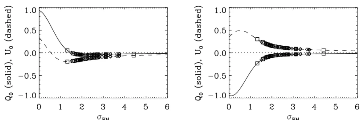
uniform polarized background so that no large-scale compo-nents inQandUremain. Figure 5 displays the oﬀsets as cal-culated from Eqs. (1) and (2) for each pointing. The solid and dashed lines denote the theoreticalQ0andU0respectively, the

symbols show theσRMin the Auriga field (diamonds) and in the Horologium field (squares). As oﬀsets also depend onφ0, the

figure shows minimal oﬀsets (forφ0 =10◦, left) and maximal

oﬀsets (forφ0 =80◦, right). The symbols denote theσRMfor pointings in the Auriga field (diamonds) and Horologium field (squares).

In the best case (φ0 = 10◦), no pointings in Auriga and

one pointing in Horologium have oﬀsets exceeding 20%, which corresponds to an error in polarization angle ε_φ of 10%. In the worst case (φ0 = 80◦), 3 pointings in Auriga (out of 35)

and 9 in Horologium (out of 25) allow oﬀsets above 20%. However, only one pointing (in Horologium) would allow oﬀ -sets higher than 27% (εφ = 14%). Therefore, if our obser-vations result from a uniformly polarized background viewed through a Faraday-modulating screen, theσRMin most point-ings in our fields is so large that missing large-scale structure leads to an error in polarization angle of less than 10%.

The magnitude of the oﬀsets can also be estimated from the variation of observed polarization angleφwith wavelength.

The observations show thatφdoes not perfectly follow the lin-ear relation φ = φ0 +RMλ2, as one would expect for pure

Faraday rotation. Oﬀsets in Qand/orU can cause deviations in the linearφ(λ2_{)-relation, so we estimated in both fields the}

oﬀsets that would minimize the observed non-linearities in the

φ(λ2_)-relation.

For this, subfields of∼1◦×1◦were selected around a point-ing center. A large-scale constantQ0 and/orU0, independent

for each frequency, were added to the data to minimize theχ2

of theφ(λ2_{)-relation. Resulting o}_ﬀ_{set values in some subfields}

had a magnitude of the same order as P in that field, which decreased the averageχ2_redby a factor of two. However, Fig. 6 shows the distribution of individual reducedχ2values per beam for a typical pointing in the Auriga field. The left plot shows reducedχ2 _{values computed with o}_ﬀ_{sets against reduced}_χ2

without oﬀsets. In the right hand panel, the histograms of χ2

without (solid line) and with oﬀsets (dotted line) are given. Oﬀsets only cause a decrease inχ2 _{in 52% of the beams,}

al-though the averageχ2_{diminishes. In other pointings, this}

per-centage ranges from 49% to 71%. Therefore, the computed oﬀ -sets do not give a real improvement of the data, and cannot be considered real missing large-scale components. Of course, this argument assumes that oﬀsets are the only agents distort-ing the linearφ(λ2_{)-relation, while depolarization mechanisms}

can yield non-linearity too. In addition, it assumes that the oﬀ -sets are constant over the subfield considered, which may not be true either. Probing smaller subfields is no solution for this problem as the number of data points becomes too small with respect to the number of free parameters.

A third argument against dominant oﬀsets in the data is the high quality of the determination of RM, i.e. a lin-earφ(λ2_{)-relation with a low}_χ2_{. Of all pixels with high enough}

polarized intensity (P > 20 mJy/beam),∼70% (in Auriga) and∼62% (in Horologium) has a reducedχ2 _<_{2. If o}_ﬀ_{sets of}

the same order of the data would exist, RMs could not be so well-determined over such a large part of the fields. For ideal data with constantP, random oﬀsets cause aχ2 >2 if the oﬀ -sets are larger than∼8%.

Finally, models of depolarization in a synchrotron-emitting and Faraday-rotating medium, which are presented in a com-panion paper (Haverkorn et al. 2004a), do not show averageQ

orUvalues>_∼10 mJy/beam (2σ).

(6)

Fig. 5.Missing large-scale structure inQ(solid line) andU(dashed line) for a Faraday screen with a GaussianRMdistribution with widthσRM

andP0 =1, assuming that the oﬀsets are constant over the field. Diamonds denoteσRM observed in the pointings of the Auriga field, squares

are the pointings of the Horologium field. Oﬀsets depend on the intrinsic polarization angleφ0, shown are the best- and worst-case scenario for

φ0=10◦(left) andφ0=80◦(right).

Fig. 6.The influence of oﬀsets on reducedχ2_{in a subfield of Auriga.}

Left: reducedχ2_{distribution of linear}_φ₍_λ2_{)-relation with best-fit o}_ﬀ

-sets against values of reducedχ2 _{without o}_ﬀ_sets._Right_{: distribution}

of reducedχ2_{with computed o}_ﬀ_{sets (dotted line) and without o}_ﬀ_sets

(solid line).

considerable undetected large-scale structure due to the miss-ing short spacmiss-ings is unlikely.

This conclusion can also be checked with absolutely cali-brated polarized intensity maps at 408 MHz by Berkhuijsen & Brouw (1963). This frequency is close enough to 350 MHz to allow comparison, although the polarized intensity at 408 MHz is expected to be slightly higher because the polarization hori-zon is further away at this frequency. We have smoothed our data to the 2◦ FWHMof Berkhuijsen & Brouw, and derived any missing large-scale structure by comparing the two data sets. The polarized brightness temperatures at 408 MHz at the positions of the Auriga and Horologium fields are 1.8 K and 2.7 K, respectively. Using a power law spectral index of 2.7, this corresponds to 2 K and 3 K at 350 MHz. The polarized brightness temperatures derived from the smoothed data are 0.07 K and 0.12 K, respectively. Converting from Kelvin to Jansky per beam (see Table 1) and taking into account that oﬀsets in Qand U are on average a factor √2 smaller than those inP, this means that any missing large-scale components in StokesQandU are smaller than 10.6 mJy beam−1_{for the}

Auriga region, and 13.7 mJy beam−1_{for Horologium. For both}

fields, this corresponds to about 2 to 3 signal-to-noise in Q

andU, although it is not known what the influence of the dif-ference in polarization horizon is. We conclude that these data

are not in disagreement with our conclusion that missing large-scale structure does not play a major role in these observations. Therefore, the structure in polarized intensity must be due wholly to depolarization mechanisms. For a pure Faraday screen the only kind of depolarization that is possible is beam depolarization, because the observed values ofRMimply that bandwidth depolarization is not important, while depth de-polarization requires that the rotating medium emits as well. However, beam depolarization can only explain structure inP

on beam-size scales. Therefore we are led to consider the more realistic situation in which we observe a polarized background that is modulated by a layer that both causes Faraday rotation, and emits synchrotron radiation. Note that the argument which limits the importance of oﬀsets through the width of the dis-tribution of observedRMs applies equally to a pure Faraday rotating screen and to a rotating and emitting screen.

The only way in which oﬀsets could play a rôle is if there were a layer in front of the rotating and emitting screen which emits polarized radiation that is constant over the primary beam of our observations. A foreground-oﬀset decreases the degree of polarization with a constant factor and can contribute a con-stantRM component which cannot be derived from the data. However, a uniformly polarized foreground cannot influence the width of observed RM distribution or induce small-scale depolarization. Judging from earlier single-dish data ofRMin the regions of the Auriga and the Horologium region (Bingham & Shakeshaft 1967; Spoelstra 1984), we conclude that a possi-ble undetectedRMcomponent on scales>_∼1◦, if present at all, must be very small.

4. Depolarization canals

(7)

Fig. 7.Frequency dependence of the depth of the canals, in the Auriga region (top) and Horologium region (bottom).Pis the average over all canal-pixels, and in each plot the canals were defined in an other frequency band, at 341, 349, 355, 360, and 375 MHz from left to right. The prediction forP(λ2_{) if all canals were caused by beam depolarization due to a change in}_RM_{is shown in dashed lines, from bottom to top for}

∆RM ≈2.1, 6.3 rad m−2_(i.e._∆_φ₌₉₀◦_,₂₇₀◦_{). The prediction for}_P₍_λ2_{) if the canals were caused by di}_ﬀ_{erential Faraday rotation are shown}

dotted for 2RMcλ2=nπforn=1,3 and 5.

(Haverkorn et al. 2000). This characteristic behavior can be explained by two mechanisms:

1. The canals can denote a boundary between two regions which each have approximately constant polarization an-gle, but between which there is a diﬀerence in polarization angle of ∆φ = (n+1/2)180◦ (n = 0,1,2, . . .). This will cause almost total depolarization through vector addition, if the polarized intensities on either side of the boundary are essentially identical (Haverkorn et al. 2000). The resulting canal is, by definition, one beam wide.

2. A medium containing a uniform magnetic field, thermal electrons and cosmic-ray electrons depolarizes polarized radiation by means of diﬀerential Faraday rotation. In this case, the observed polarized intensity is

P=P0

sin(2RMλ2₎

2RMλ2

(3)

(Burn 1966; Sokoloﬀet al. 1998), where P0 is the

polar-ized intensity observed atλ→ 0. A linear gradient inRM

would produce long narrow depolarization canals at a cer-tain valueRMcwhere 2RMcλ2 =nπ. Across every null in

the sinc-function, the polarization angle changes by 90◦. We will attempt to estimate the importance of each of the two mechanisms in our observations.

4.1. Frequency dependence of canals

If the canals are due to beam depolarization, there are two ex-treme possibilities for the origin of the angle change ∆φ = (n+1/2) 180◦: it can be due to either anRM change across a canal of (n+1/2) 180◦/λ2_{, or to an intrinsic angle di}_ﬀ_erence

of∆φ0=(n+1/2) 180◦. These two extremes cannot be

distin-guished from observations at a single frequency. However, one

would expectPin the canals to vary with frequency if theRM

changes across a canal, while the depth of a canal should be constant for a∆φ0. If, on the other hand, the canals are caused

by diﬀerential Faraday rotation, P in a canal should change with frequency according to Eq. (3).

We have tested the frequency dependence of the depth of the canals as follows. Canals are defined as sets of “canal-pixels”. A pixel is defined as a “canal-pixel” if the polarized intensity is low (P < 2 times rms noise) and P on diamet-rically opposed sides of that pixel, one beam away, is high (P > 5 times rms noise). The high-Ppixels surrounding the canal-pixel can be oriented horizontally, vertically or diago-nally. No further assumptions regarding the length of canals are made; therefore a single pixel with lowPthat is no part of a canal but is surrounded by highPpixels, is also defined to be a canal-pixel.

Sets of canal-pixels are evaluated for each frequency sep-arately, so that five sets of canal-pixels result. The averageP

in each set of canal-pixels is computed at all frequencies. In Fig. 7, we plot the average values ofPagainstλ2 for the five sets of canal-pixels (where canals are defined at one of the frequencies) in the Auriga and Horologium regions. In each panel in Fig. 7, i.e. for each frequency, and both in Auriga and Horologium, the wavelength in which the canals are selected has the lowest averageP, withPincreasing with|∆λ2_|_{, i.e. the}

canals decrease in depth at the other wavelengths. This rules out the possibility that the canals are caused by a change in in-trinsic angle, confirming the conclusion from the non-detection ofIthat the background polarized intensity is smooth.

The dashed lines show the predictions ofP(λ2_{) for canals}

that are caused by beam depolarization, and are due to a change inRM (with∆RM =2.1 and 6.3 rad m−2_{, respectively). The}

(8)

Fig. 8.Distribution of∆RMcacross canals and the absoluteRMcat the canal position (as estimated from its neighbors). Canals are defined at

frequencies 341, 349, 355, 360, and 375 MHz from left to right. Top panels show the Auriga region and bottom panels the Horologium region. OnlyRMcvalues whereχ2red<2 andP>20 mJy/beam are used. In the∆RMcplots, dotted vertical lines are∆RMcvalues where∆φacross a

canal would be±90◦,±270◦or±450◦. In theRMcplots, the dotted vertical lines are values where 2RMcλ2=nπ.

from Eq. (3). Both predictions have arbitrary polarized intensi-ties. Therefore, the scaling of the models contains no physical information, and is adjusted to fit the data.

The accuracy of the model predictions can be judged by the shape of the predicted lines, which is typical of the responsible depolarization process. Furthermore, the same scaling should be used for each frequency. Judging solely from the shape of the lines, the prediction of diﬀerential Faraday rotation seems to make a fit somewhat better than that of beam depolarization, but not by much. This is not totally unexpected, because it is probable that a combination of both processes is at work in the majority of pixels.

4.2.

RM

and

∆RM

values in canals

Canals due to beam depolarization are caused by a specific change inRM across a canal∆RMc =(n+1/2)π/λ2. On the

other hand, canals caused by diﬀerential Faraday rotation are

determined by a specific absoluteRMc = nπ/(2λ2). With the

sets of canal-pixels defined in the previous subsection, we de-fine∆RM =RM1−RM2, where 1 and 2 are high-Ppixels on

opposite sides of the canal. Then the RM at the canal-pixel is estimated asRM=(RM1+RM2)/2. The observed distributions

of∆RMandRMare shown in Fig. 8. Both∆RMandRM distri-butions show peaks at the values that will produce canals, and the observations do not show perfect agreement with either of them. Note that canals with angle changes∆φ <_∼90◦ have ac-companying∆RMs orRMs slightly diﬀerent from canals with ∆φ = 90◦ and therefore broaden the peaks. Noise inRM has the same eﬀect.

4.3. Position shift of the canals with frequency

Diﬀerential Faraday rotation causes total depolarization at all positions where RM = RMc. This means that

(9)

large-scale gradient observed in the Auriga region, this indi-cates that the canal should move with position over∼5 beams from 341 MHz to 375 MHz. Instead, canals move at maximum 3 pixels from 341 to 375 MHz, which is about 0.5 beam.All

gradients inRMwould have to be larger than∼1 rad m−2_per

beamto position the canals in the 5 frequencies within half a beam from each other. Such a gradient is certainly possible lo-cally, although this high gradient would have to extend over a large part of the field in order to explain the long and straight canals. Furthermore, if such large gradients are present in the medium, we would expect lower gradients as well. These lower gradients would give canals that shift position with frequency significantly, which we do not observe.

4.4. Shape of the canals

The shape of the decline inPacross a canal, or the “steepness” of a canal, gives a lower limit to the abruptness of the change in polarization angle across a canal, as can be seen in Fig. 9. Here a one-dimensional example is given of a change in polarization angle∆φ = 90◦ (left) and the corresponding change inP af-ter convolution with the telescope beam (right). The narrowest

Pprofile is achieved when the change in angle is on a length scale smaller than about one fifth of the beam.

In Fig. 10, the steepest canals found in the data are shown. In this figure the top plots give a one-dimensional cross-cut ofP

across three canals against position, for all frequencies. The frequencies in which the canals were defined were 341 MHz, 355 MHz and 349 MHz respectively, and the canals were se-lected for their steepness. The bottom plots give only the P

distribution across the canal at the frequency at which it was defined (solid line). Superimposed in dashed lines is theP dis-tribution of the model of Fig. 9 for the steepest angle change convolved with the synthesized beam. Less steep angle changes give less steepPprofiles and worse fits to the data. An interpre-tation of these (specifically selected) steep canals in terms of diﬀerential Faraday dispersion is diﬃcult, because the canals would have to be much more closely spaced than observed. Beam depolarization predicts a change in depth of the canals across the frequency bands of about 20%, in agreement with the observations.

4.5. Canals due to beam depolarization

We conclude that the dominant process creating one-beam wide canals of almost complete depolarization is most likely beam depolarization. In this case, abruptRMchanges have to be present in the medium. It may seem fortuitous that only

RM gradients of the right magnitude to make canals would

across a canal with diﬀerent gradients (left). Convolution ofQandU

gives thePdistribution as shown right for the 3 gradients. The width of the beam is 12 pixels.

Fig. 10.Measures shapes of the deepest canals.Upper plots: examples of observed one-dimensionalPdistributions in the Horologium region for five frequencies, where the deepest canal is observed at 341, 355 and 349 MHz respectively.Lower plots: the samePdistribution for the deepest canal as above (solid) and the best fit according to the model of Fig. 9. ThePprofile is so steep that the change in angle that causes the canal must be on scales of an arcminute or smaller.

exist. However, this is not the case:RMgradients of any mag-nitude are likely to occur in the medium, but only theRM gra-dients that cause ∆φ ≈ 90◦ yield a visible signature in P. BecauseRM is an integral along the line of sight, it is diﬃ -cult to see what physical process would be responsible for this. However, numerical models of a magneto-ionized ISM show thatRMgradients steep enough to produce canals at 350 MHz are common (Haverkorn & Heitsch 2004). The relatively low

RM gradient needed to make a canal at 350 MHz, as com-pared to 1.4 GHz observations, could explain why canals are abundant in these WSRT observations, but are much less com-mon at 1.4 GHz (Uyanıker et al. 1998). Nevertheless, Figs. 7 and 8 show that beam depolarization certainly is not the whole explanation.

(10)

to almost zero would then indicate a very uniform medium in both magnetic field and electron density. Sokoloﬀet al. (1998) showed that an exponential asymmetric slab causes non-zero minima for the canals, which even disappear completely in a turbulent medium. Small-scale structure in observedRM indi-cates that small-scale structure in magnetic field and/or electron density is abundant, so that a uniform medium needed for deep canals in the diﬀerential Faraday rotation interpretation is un-likely. However, Shukurov & Berkhuijsen (2003) argue that the canals they observed at 1.4 GHz in M31 are best explained as due to depth depolarization.

5. Conclusions

Small-scale structure in the linearly polarized component of the diﬀuse Galactic synchrotron emission is seen in almost ev-ery direction. Mostly, this structure is not correlated with total emission, and therefore cannot be due to small-scale structure in emission. Instead, the polarization angleφis Faraday-rotated in the magneto-ionic medium through which the linearly po-larized radiation propagates. However, the structure in polar-ized intensityPcannot be produced by Faraday rotation alone (which only rotatesφ), but there are several other processes responsible for this. First, instrument-related eﬀects produce structure inP, such as large-scale components in the radiation that are undetectable with an interferometer, depolarization due to variation in angle within the telescope beam, or over the fre-quency band width. Furthermore, physical depolarization pro-cesses in the ISM can cause depolarization if Faraday rotation and synchrotron emission occur in the same medium.

In this paper, we have discussed these processes and gauged their relative importance in two sets of observations made with the Westerbork Synthesis Radio Telescope (WSRT).

Undetectable large-scale components in StokesQand/orU

measurements can create structure inP, and prohibit the correct determination of rotation measure. However, we showed that in our fields, the observed range in rotation measure is so large that oﬀsets cannot play a significant rôle.

Narrow one-beam-wide canals of depolarization can be caused by beam depolarization or diﬀerential Faraday rotation. Our observations suggest that beam depolarization is the dom-inant mechanism responsible for the canals at 350 MHz, al-though depth depolarization is likely to contribute.

Acknowledgements. We wish to thank R. Beck, E. Berkhuijsen and J. Tinbergen for helpful discussions. The Westerbork Synthesis Radio Telescope is operated by The Netherlands Foundation for Research in Astronomy (ASTRON) with financial support from the Netherlands Organization for Scientific Research (NWO). MH acknowledges sup-port from NWO grant 614-21-006.

Appendix A: Offsets for a non-emitting Faraday screen

First we consider the situation of a small-scale Faraday screen, i.e. of a constant polarized background emission that undergoes Faraday rotation while propagating through a magneto-ionized

medium. In this case, small-scale structure in polarization an-gle is created by the Faraday rotation, while the polarized in-tensity remains unaltered. We assume a uniform polarization backgroundP0 =P0 exp(−2iφ0), whereφ0is the intrinsic

po-larization angle. Assuming that the oﬀsets can be approximated by a constant over the whole field of observation, the expected oﬀsets can be derived depending on theRMdistribution in the screen. We consider the case in which the Faraday screen con-sists of cells with randomRMrdrawn from a GaussianRM

dis-tribution of widthσRMand thus Faraday-rotates the background polarization angle on small scales. The oﬀsets are then the nor-malized mean of the polarized emission P0 = P0 exp(−2iφ0)

weighted with the GaussianRMdistribution:

Poﬀsets=

_∞

−∞P0e2i(φ0+RMrλ

2₎

n(RMr) dRMr

_∞

−∞n(RMr) dRMr

(A.1) where n(RMr)=e−RM

2 r/2σRM2.

This expression is independent of the angular length scale of the structure inRM, as long as the length scale is small enough with respect to the path length to have a Gaussian distribution ofRMs. This yields the oﬀsetsQ0andU0

Q0=A

cos(2φ0)−

1 √

πsin(2φ0)F

(A.2)

U0=A

sin(2φ0)−

1 √

πcos(2φ0)F

(A.3)

whereF=

√

2σRMλ2

0

et2dt and A=P0e−2σRM

2_λ4

.

The oﬀsets depend highly non-linearly upon the width of the randomRM distributionσRM. The exact values can be easily calculated analytically for two extremes:

a) The width of the φ-distribution σφ = σRMλ2 >∼ π, or largeσRM:

e−2σRM2λ4→₀ ⇒ _Q

0=U0=0.

The observed distribution of polarization angles is random, thereforeQandUare centered around zero and there is no undetected large-scale structure.

b) σRMand accompanyingσφare so small thatσRMλ21:

e−2σRM2λ4→₁ ⇒ 

_UQ0₀ =₌P_P0₀ cos(2_sin(2_φφ₀0₎)_.

Here the subtracted component is equal to the uniform component of the polarization vector. The observed polar-ized intensity is much lower than the true polarpolar-ized inten-sity because of these large oﬀsets.

A constant background rotation measureRMucan be

incorpo-rated by replacingφ0in the equations byφu=φ0+RMuλ2, but

(11)

Burn, B. J. 1966, MNRAS, 133, 67

Duncan, A. R., Reich, P., Reich, W., & Fürst, E. 1999, A&A, 350, 447 Fletcher, A., Berkhuijsen, E. M., Beck, R., & Shukurov, A. 2004,

A&A, 414, 53

Gaensler, B. M., Dickey, J. M., McClure-Griﬃths, N. M., et al. 2001, ApJ, 549, 959

Gardner, F. F., & Whiteoak, J. B. 1966, ARA&A, 4, 245

Gray, A. D., Landecker, T. L., Dewdney, P. E., et al. 1999, ApJ, 514, 221

Haverkorn, M., & Heitsch, F. 2004, A&A, 421, 1011

Haverkorn, M., Katgert, P., & de Bruyn, A. G. 2000, A&A, 356, L13

299, 189