RECONCILING THE OBSERVED STAR-FORMING SEQUENCE WITH
THE OBSERVED STELLAR MASS FUNCTION
Joel Leja1, Pieter G. van Dokkum1, Marijn Franx2, and Katherine E. Whitaker3,4
1Department of Astronomy, Yale University, New Haven, CT 06511, USA 2Leiden Observatory, Leiden University, PO Box 9513, NL-2300 AA Leiden, The Netherlands 3Astrophysics Science Division, Goddard Space Flight Center, Code 665, Greenbelt, MD 20771, USA
Received 2014 June 17; accepted 2014 October 31; published 2015 January 7
ABSTRACT
We examine the connection between the observed star-forming sequence (SFR∝Mα) and the observed evolution of
the stellar mass function in the range 0.2< z <2.5. We find that the star-forming sequence cannot have a slopeα
0.9 at all masses and redshifts because this would result in a much higher number density at 10<log(M/M)<11 byz=1 than is observed. We show that a transition in the slope of the star-forming sequence, such thatα=1 at log(M/M)<10.5 andα=0.7–0.13z(Whitaker et al.) at log(M/M)>10.5, greatly improves agreement with the evolution of the stellar mass function. We then derive a star-forming sequence that reproduces the evolution of the mass function by design. This star-forming sequence is also well described by a broken power law, with a shallow slope at high masses and a steep slope at low masses. Atz=2, it is offset by∼0.3 dex from the observed star-forming sequence, consistent with the mild disagreement between the cosmic star formation rate (SFR) and recent observations of the growth of the stellar mass density. It is unclear whether this problem stems from errors in stellar mass estimates, errors in SFRs, or other effects. We show that a mass-dependent slope is also seen in other self-consistent models of galaxy evolution, including semianalytical, hydrodynamical, and abundance-matching models. As part of the analysis, we demonstrate that neither mergers nor hidden low-mass quiescent galaxies are likely to reconcile the evolution of the mass function and the star-forming sequence. These results are supported by observations from Whitaker et al.
Key words: galaxies: evolution – galaxies: high-redshift – galaxies: luminosity function, mass function – galaxies: star formation
1. INTRODUCTION
The redshift evolution of the stellar mass function is a fundamental observable of galaxy evolution because it directly measures the stellar mass buildup of galaxies. Recently, it has been measured with unprecedented precision by a number of wide, deep near-infrared surveys (Muzzin et al.2013; Ilbert et al.
2013; Moustakas et al.2013; Davidzon et al. 2013; Tomczak et al.2014). These surveys are revealing new frontiers in galaxy evolution; for example, the FourStar Galaxy Evolution Survey (ZFOURGE) is mass-complete to log(M/M)=9.0 atz=2 for both star-forming and quiescent galaxies (Tomczak et al.
2014). This impressive depth has revealed that simple Schechter fits are not a good representation of the mass function in the high-redshift universe.
The observed relationship between the star formation rate (SFR) and stellar mass of star-forming galaxies (the “star-forming sequence”), measuring the derivative of the mass buildup of galaxies, has also been of great interest in the literature (Brinchmann et al.2004; Noeske et al.2007; Daddi et al.2007; Peng et al.2010; Karim et al.2011; Whitaker et al.
2012; Guo et al.2013a; Speagle et al.2014). Recently, this has been measured robustly out to a high redshift and over a wide variety of SFR indicators (Oliver et al.2010; Wuyts et al.2011; Karim et al.2011; Whitaker et al.2012) and further extended down to low stellar masses and star formation rates in the local universe (Huang et al. 2012). Much work has been done to bring these different SFR indicators into agreement (Wuyts et al.
2011), and there has been some success in putting these many studies into a consistent framework (Speagle et al.2014).
4 NASA Postdoctoral Program Fellow.
While there has been great progress in reducing errors that are due to limited depth and field-to-field variations, the interpretation of these data is still subject to systematic uncertainties. Stellar mass measurements, particularly at higher redshifts, are uncertain by at least a factor of two because of unknowns such as emission line contributions, star formation histories, dust content, and metallicities (Marchesini et al.2009; Conroy et al.2009; Behroozi et al.2010; Mitchell et al.2013). Although in principle these stellar mass measurements can be calibrated with dynamical masses, only a handful of galaxies atz ∼ 2 have reliable stellar velocity dispersions so far (van de Sande et al. 2013; Belli et al.2014). Star formation rates also suffer from uncertainties, particularly in low-mass galaxies at high redshift, because of flux limits, systematic differences between SFR indicators, and selection effects (Mitchell et al.
2014; Speagle et al.2014).
Given these systematic uncertainties, it is important to test whether the observed star-forming sequence and the observed evolution of the mass function are consistent with one another. A version of this phenomenological test was applied by Bell et al. (2007) and has been implicitly performed by several studies since (Drory & Alvarez2008; Peng et al.2010; Behroozi et al. 2013c). Most recently, Weinmann et al. (2012) has showed that in order for the star-forming sequence to be consistent with the number density evolution of low-mass galaxies atz <1, either (1) for SFR∝Mα,αmust be greater
possible by the ultra-deep ZFOURGE mass functions (Tomczak et al.2014).
We use the ZFOURGE mass functions to take a fresh look at the consistency between the stellar mass function and the star-forming sequence in the range 0.2< z <2.5. We compare this to the star-forming sequence from Whitaker et al. (2012), which has been mapped with deep medium-band near-infrared (NIR) imaging and consistent UV+IR SFR indicators in the range 0< z <2.5.
The layout of the paper is as follows. In Section2, we con-struct a smooth analytical description of the redshift evolution of the stellar mass function. In Section3, we build a model to compare the growth of the mass function implied by differ-ent low-mass extrapolations of the star-forming sequence to the observed growth of the mass function, and based on this com-parison, we postulate a new functional form for the star-forming sequence. Section4discusses the implications of our results and the remaining uncertainties, and the conclusion is in Section5. We use a standardΛCDM (cold dark matter) cosmology, with ΩM=0.3,ΩΛ=0.7, andh=0.7, and we use a Chabrier initial
mass function (IMF).
2. THE OBSERVED EVOLUTION OF THE MASS FUNCTION
We adopt mass functions from the ZFOURGE survey, measured in the range 0.2< z <2.5 (Tomczak et al. 2014). ZFOURGE is the deepest measurement of the stellar mass function to date, and it makes use of ground-based near-infrared medium-bandwidth filters that improve the accuracy of photo-metric redshifts (van Dokkum et al.2009). The survey also incor-poratesHSTimaging from the Cosmic Assembly Near-infrared Deep Extragalactic Legacy Survey (CANDELS; Grogin et al.
2011; Koekemoer et al.2011). ZFOURGE uses the CANDELS H160filter as the detection criteria. ZFOURGE imaging covers an area of 316 arcmin2, and the ZFOURGE catalogs include data from the wider but shallower NEWFIRM Medium-Band Survey (NMBS; Whitaker et al.2011) to tighten the constraints at the massive end. Star-forming and quiescent galaxies are sep-arated by their rest-frameUVJcolors as described in Williams et al. (2009).
We supplement the ZFOURGE mass functions with low-redshift mass functions measured from Sloan Digital Sky Survey (SDSS) GALEX data (Moustakas et al. 2013). These cover the redshift range 0.02< z <0.2 and have ugriz photometry and spectroscopic redshifts from the SDSS Data Release 7 (Abazajian et al.2009). They includeJHKs photometry from the Two Micron All Sky Survey (2MASS) Extended Source Catalog (Jarrett et al.2000) and photometry at 3.4 and 4.6μm from the WISE All-Sky Data Release (Wright et al.2010). Star-forming and quiescent galaxies are separated via UV luminosity as measured by theGalaxy Evolution Explorer(GALEX; Martin et al.2005).
We use these data to construct an analytical description of the evolution of the stellar mass function with time. We aim to smoothly parameterize the redshift evolution of the stellar mass function asφ(M, z). Historically, the stellar mass function has been fit with a Schechter function (Schechter1976). Recently, however, deeper measurements of the stellar mass function have shown that a double Schechter function is necessary to describe the steepening of the slope at masses below 1010M
(Baldry et al.2008; Li & White2009; Drory et al. 2009; Moustakas et al.2013; Muzzin et al.2013; Ilbert et al.2013; Tomczak et al.
2014). The logarithmic form of the double Schechter function is
φ(M)dM=ln(10) exp (−10(M−M∗))10(M−M∗)
[φ1∗10(M−M∗)α1+φ∗
210(
M−M∗)α2]dM, (1)
where, in this equation, M = log(M/M) and M∗ =
log(M∗/M). While in principle each component of the dou-ble Schechter could have a separateM∗, the data are consistent with a single value of M∗ for each component of the double Schechter function.
It is difficult to simply use the best-fit Schechter parameters to construct a smooth model for the evolution of the mass function. However, because of degeneracy between parameters in a double Schechter function, an unconstrained chi-squared minimization leads to Schechter parameters that do not evolve smoothly with redshift. We have found that simply interpolating in redshift between the best-fit Schechter parameters will introduce spurious increases and decreases in number density between the observed redshift windows.
To avoid these numerical artifacts, we refit constrained double Schechter functions separately to the observed star-forming, quiescent, and total mass functions in each redshift window. We limit degenerate solutions by fixing the faint-end slopes to the best-fit values at 0.5 < z <0.75 from Tomczak et al. (2014), which are
total:α1= −0.39
α2= −1.53
quiescent:α1= −0.10
α2= −1.69
star−forming:α1= −0.97
α2= −1.58.
We follow Drory & Alvarez (2008) in fitting second-order polynomials to the redshift evolution of the remaining best-fit Schechter parameters, namelyφ1,φ2, andM∗. We then refit
φ1, φ2,andM∗, constraining them to be within 40% of the best-fit second-order polynomials. We perform this best-fit iteratively, constraining the best-fitφ1,φ2, andM∗to be increasingly close to the second-order polynomials during each fit.
The goals of this procedure are to (1) reproduce the evolution of the observed mass function in the observed redshift windows and (2) enforce smooth, monotonic evolution of the mass function between observed redshift windows. This iterative approach maximizes the effectiveness of the polynomial fits in building a smooth model for redshift evolution of the stellar mass function, though we recognize that it does not necessarily guarantee a unique solution.
The resulting redshift evolution of the Schechter parameters is
total: log (φ1)= −2.46 + 0.07z−0.28z2
log (φ2)= −3.11−0.18z−0.03z2
log (M∗/M)=10.72−0.13z+ 0.11z2 quiescent: log (φ1)= −2.51−0.33z−0.07z2
log (φ2)= −3.54−2.31z+ 0.73z2
log (M∗/M)≡10.70
star−forming: log (φ1)= −2.88 + 0.11z−0.31z2
log (φ2)= −3.48 + 0.07z−0.11z2
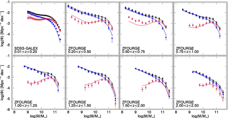
Figure 1.Redshift evolution of the stellar mass function for all (black), star-forming (blue), and quiescent (red) galaxy populations. The filled circles are data from the ZFOURGE mass functions (Tomczak et al.2014) and SDSS–GALEX(Moustakas et al.2013), and the lines are the smooth model forφ(M, z), constructed as described in Section2. The smooth model broadly reproduces the evolution of the stellar mass function in the range 0.2< z <2.5.
Because we find no significant redshift evolution in the quiescent
M∗, we fix it to its average value.
The parameterized mass function growth,φ(M, z), is com-pared directly with the measured ZFOURGE mass functions in Figure1. There is overall good agreement with the observed mass function. Noticeably, the observed number density of low-mass quiescent galaxies is underpredicted by∼0.3 dex at 0.5< z < 0.75 and overpredicted by∼0.2 dex at 0.2 < z < 0.5. The data show negligible evolution in the number density of low-mass quiescent galaxies between these two redshift win-dows. However, there is still significant evolution fromz =1 toz =0.35 and fromz= 0.625 toz = 0.1, and the smooth evolution in the model reflects the broader trend of declining number density in low-mass quiescent galaxies with increasing redshift. In practice, this offset has a negligible effect on our conclusions: the quiescent mass function is only used to calcu-late the fraction of star-forming galaxies as a function of mass, and star-forming galaxies dominate at low masses regardless of the normalization offset.
In the following analysis, we extrapolate the stellar mass function to below the nominal stellar mass completeness when necessary. The assumed shape of the stellar mass function below the observed completeness limit does not have a significant effect on our results, however.
3. THE EVOLUTION OF THE MASS FUNCTION AS IMPLIED BY THE STAR-FORMING SEQUENCE
We now compare the evolution of the mass function, as implied by the star-forming sequence, to the observed evolution of the mass function, as parameterized in Section2. We begin by describing the model that connects the star-forming sequence to the growth of the mass function. We also include a simple model for the effect of galaxy mergers on the evolution of the
mass function. We then examine the effects of applying different star-forming sequences to the mass function.
3.1. Model for the Growth of the Mass Function
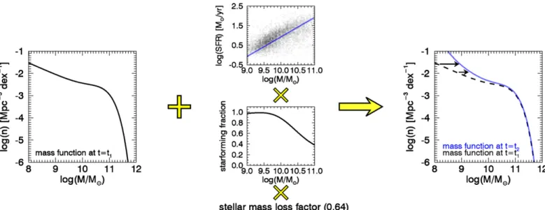
We implement a model to describe the time evolution of the mass function that is due to the observed star-forming sequence. A schematic of this model is shown in Figure2. We also include a simple model for galaxy mergers.
3.1.1. Growth of the Mass Function due to Star Formation
At each redshift step, mass is added to the mass function by star formation. Star formation will cause the mass function to shift to the “right” with time. At fixed mass, galaxies have a range of star formation rates (van Dokkum et al.2011). However, when describing the evolution of the mass function, the complex distribution of star formation rates can be reduced to the average star formation rate as a function of mass (discussed further in Section4.6.1).
In general, each bin of the mass function contains a mix of star-forming and quiescent galaxies. Adopting this division, the rate of mass addition due to star formation in each bin of the mass function is given by
˙
Mavg=
φsfM˙sf+φquM˙qu
φsf+φqu , (2)
Figure 2.Schematic representation of the model adopted to predict the evolution of the stellar mass function that is due to the star-forming sequence. We calculate the mass added to each bin of the mass function between time steps by multiplying the SFR stellar mass relationship by the fraction of star-forming galaxies as a function of stellar mass and by a constant factor of 0.64 to correct for passive stellar evolution. The addition of mass via star formation will shift the stellar mass function “to the right,” whereas mergers will shift it “down and to the right.”
lower thanUVJ-selected star-forming galaxies and thus can be safely neglected (Fumagalli et al.2014).
We definefsf, the fraction of star-forming galaxies, to be the following:
fsf(M, z)= φ(M, z)sf
φ(M, z)qu+φ(M, z)sf. (3)
We calculatefsf(M, z) directly from our smoothed model for the evolution of the mass function and fit it with
fsf=f0−(f0−0.2) tanh[a(log(M/M)−b)]. (4)
The fit is restricted to 9<log(M/M) <11, where the mass function is mass-complete and the effects of cosmic variance are minimized at the high-mass end (Tomczak et al.2014). By construction, at high masses the adopted star-forming fraction asymptotically approachesfsf=0.2, consistent with studies of brightest cluster galaxies (BCGs) in the local universe (Bauer et al.2013; Oliva-Altamirano et al.2014). At low masses, the star-forming fraction asymptotes tof0; the typical best-fit value off0is∼0.9.
We takeM˙sfto be ˙
Msf(M, z)=SFR(M, z)×(1−R), (5)
where SFR(M, z) is the star formation rate implied by the star-forming sequence. The variableRis the fraction of mass ejected from a stellar population during the course of passive stellar evolution, primarily due to winds and outflows. In general,
R = R(t), starting at R = 0 when the stellar population is formed and ending at R = 0.36 after ∼10 Gyr (assuming a Chabrier IMF). However, because most of the mass loss occurs within the first hundred million years, we approximate mass loss as instantaneous, fixingRto 0.36 (see Section4.6.2for further discussion of this approximation). The final equation for the average growth rate of the mass function due to star formation is thus
˙
Mavg=SFR(M, z)×fsf(M, z)×(1−R). (6)
3.1.2. Growth of the Mass Function due to Mergers
The framework described so far models the growth of the mass function that is solely due to star formation. The other physical process that can change the number density of galaxies is galaxy mergers. Specifically, mergers affect the mass function in two ways: (1) they directly decrease the number density of galaxies and (2) they contribute to the stellar mass growth of galaxies.
We model both of these effects. We measure the merger rate measured directly from the Guo et al. (2013b) semian-alytical model (SAM) based on the Millenium-II simulation (Boylan-Kolchin et al.2009). At each snapshot in redshift, we measure the rate at which galaxies merge with more massive galaxies than themselves, which is the rate of “destruction” by mergers. This is shown as a function of mass in Figure11in AppendixA. For low-mass galaxies, this rate varies by 1%–2% per snapshot in redshift but broadly declines from ∼7% per gigayear atz ∼ 2 to∼3% per gigayear in the local universe. This is consistent with observed destruction rates of∼10% per gigayear (Bridge et al. 2010; Lotz et al. 2011), though other studies that determine merger rates based on galaxy morphol-ogy find destruction rates that are three to five times higher (Conselice2014). We show in Section4.5that our conclusions are robust to changing the destruction rate.
(a) (b) (c)
(d) (e) (f)
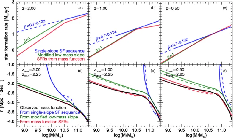
Figure 3.Panels (a)–(c) show the different adopted relationships between stellar mass and star formation rate. The observed star-forming sequence (blue) is from Whitaker et al. (2012), with the extrapolation below their mass-completeness limit marked with a dashed line. The modified low-mass slope (green) uses the Whitaker et al. (2012) slope above log(M/M)=10.5 and a slope of unity below log(M/M)=10.5. The SFR from the ZFOURGE mass functions is constructed as described in Section3.2.3for stellar masses above the ZFOURGE mass-completeness limits and is fit with a broken power law. Panels (d)–(f) show the observed ZFOURGE mass function (black), along with the mass functions grown by the corresponding star formation rates fromz=2.25. The growth of the mass function with mergers applied is shown with a dashed line. Without a steep low-mass slope for the star-forming sequence, the number density of galaxies is quickly overpredicted.
3.2. Modeling the Growth of the Mass Function with Different Star-forming Sequences
In this section, we compare the effects of using three different star-forming sequences to grow the mass function. We start the simulation atz=2.25 with the observed mass function. In each time step, we then evolve the mass function according to the model described in Section3.1and compare it to the observed mass function. The resulting growth of the mass function, with and without mergers, is illustrated in Figure3, along with the corresponding star-forming sequences. We describe the adopted star-forming sequences and their corresponding effect on the evolution of the mass function below.
3.2.1. The Observed Star-forming Sequence
We first use the observed star-forming sequence from Whitaker et al. (2012) to model the growth of the stellar mass function. Whitaker et al. (2012) measure stellar masses and pho-tometric redshifts from NMBS, which combines photometry in five near-infrared medium-band filters with publicly available imaging from 0.15–8μm (Whitaker et al.2011). They use a com-bination ofSpitzer-MIPS and UV imaging to determine SFRs in a uniform manner in the range 0< z <2.5. Star-forming galax-ies are defined by their rest-frameUVJcolors. We note that the ZFOURGE stellar mass function uses the same colorcolor cut and also uses the NMBS imaging in the derivation of their stellar masses. Thus, the mass function and the star formation rates are measured, to a large extent, from the same galaxies, which will
minimize the effect of systematic differences in stellar masses between these two data sets.
Whitaker et al. (2012) provide the following single power-law fit to the median5SFR of star-forming galaxies:
log(SFR)=α(z)(log(M/M)−10.5) +β(z), (7)
withα(z) = 0.70–0.13z andβ(z) = 0.38 + 1.14z−0.19z2. Because of incompleteness at low masses and low star formation rates, the slope of the star-forming sequence at low stellar mass is not well constrained in this study. For reference, the mass-complete limit for NMBS is log(M/M)∼10.65 atz=2.25 and log(M/M)∼10 atz=1.25, and the SFR-complete limit for Whitaker et al. (2012) is ∼40Myr−1 at z = 2.25 and ∼15Myr−1atz=1.25. We first assume that the slope does not change as a function of mass. In the following subsection, we explore the effects of altering this assumption.
This extrapolation of the observed slope results in a dramatic rate of growth for low-mass galaxies, visible in Figure3. Byz=
2, only∼350 Myr after the simulation has started, the number density of galaxies with log(M/M)=9 is overpredicted by
5 We note that our model requires theaverageSFR of star-forming galaxies;
a factor of 100. This offset decreases as stellar mass increases: at log(M/M)=10.5, the offset is only a factor of two. The dramatic growth of these galaxies is a result of the relatively flat slope of the star-forming sequence. Atz=2, the observed slope of the star-forming sequence is 0.44, meaning that the mass-doubling timescales astdouble=M/SFR∝M−0.56. With the observed normalization of the star-forming sequence, a galaxy at log(M/M) = 8 has a doubling time of just 21 million years. The very rapid assembly of the mass function is thus a direct result of the implied high star formation rates at low masses.
When mergers are turned on, the rapid growth of low-mass galaxies causes a corresponding strong growth in high-mass galaxies. The merger growth rate is very rapid, such that by
z=1, there is actually a deficit of high-mass galaxies because they have all grown to>1011.5M
. This smooths out byz=0.5: the lower-mass galaxies grow because of star formation and mergers.
This implied rapid growth of low-mass galaxies is consistent with previous analyses from the literature (Drory & Alvarez
2008; Weinmann et al.2012). Weinmann et al. (2012) examine the difference in the evolution of low-mass galaxies between ob-servations and hydrodynamical combined with semianalytical models of galaxy evolution. In the process of this compari-son, they model the evolution of the mass function in the range 0< z <0.9 by varying the slope of the star-forming sequence. They conclude that the number density of galaxies with masses in the range 9.27 < log(M/M) < 9.77 is consistent with the observed number density if the slope of the star-forming sequence is steeper than∼0.9, though their model does not in-clude corrections for quiescent galaxies. They suggest that either a high merger rate or a steep star-forming sequence can recon-cile the mass function with the star-forming sequence. Drory & Alvarez (2008) useI-band selected mass functions and average UV star formation rates to estimate the galaxy merger rates, calculated by subtracting the evolution of the mass function that is due to star formation from the observed evolution of the mass function. They conclude that the net merger rate of low-mass galaxies must be high to be consistent with the growth of the mass function: 14% per 100 Myr at log(M/M)=9. They note that this result is sensitive to the slope of the star-forming se-quence (they adopt a slope of 0.6) and to completeness estimates at low stellar mass.
The merger rate calculated from the Guo et al. (2013b) SAM for galaxies with log(M/M)∼8 is only∼0.5–0.7% per 100 Myr, more than an order of magnitude lower than the net merger rate estimated in Drory & Alvarez (2008). Application of the SAM merger rate to the evolution of the mass function is indicated by the dashed lines in Figure3. This rate of galaxy mergers cannot compensate for the rapid growth of low-mass galaxies implied by the observed star-forming sequence.
3.2.2. A Modified Low-mass Slope
We next explore the effect of modifying the slope at low stellar masses. We postulate a simple broken power law:
log(SFR)=
α(log(M/M)−10.5) +β M >1010.5M (log(M/M)−10.5) +β M1010.5M
,
(8) with the high-mass slope and normalization fixed to the Whitaker et al. (2012) values. The low-mass slope is taken to be unity.
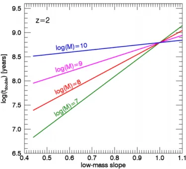
Figure 4.Timescale over which a galaxy will double its stellar mass because of star formation is plotted as a function of the low-mass slope of the star-forming sequence from Equation (8). Mass loss is taken to be a constant factorR=0.36 for consistency with the rest of the study. For flat low-mass slopes, low-mass galaxies grow at an extremely rapid rate atz=2, inconsistent with the observed growth of the mass function.
As can be seen in Figure 3, adopting this star-forming sequence effectively removes the rapid growth of low-mass galaxies. This is due to a steeper low-mass slope, which in turn implies longer mass-doubling timescales (tdouble) for low-mass galaxies. This is illustrated in Figure4, which shows the mass-doubling timescale atz = 2 as a function of low-mass slope in Equation (8). Extrapolating the observed high-mass slope of 0.44 atz=2 to low masses results in a doubling time of less than 10 million years for a galaxy of mass log(M/M)=7, compared to∼600 Myr for a slope of unity.
Thus, adopting a slope of unity at low masses results in an evolution of the mass function that compares much more favorably with the observed mass function. However, there remains an offset from the observed mass function of 0.2–0.4 dex at all masses. This offset originates atz=2 and persists to lower redshifts.
3.2.3. SFRs from the Mass Function
We now generalize the result of Section3.2.2by constructing a star-forming sequence that exactly reproduces the observed evolution of the mass function. In our simple model with no scatter in star formation rates and a slow or nonexistent merger rate, galaxy populations will evolve along lines of constant number density (Leja et al. 2013). We take a range of evenly spaced slices in number density in the range−4.3<
log(ncum/Mpc3) < −1.7 and calculate M˙(M) directly from
φ(M, z). We apply the inverse of the corrections for star-forming fraction and mass loss described above to turn this into a star-forming sequence (see Figure5).
We then perform a least chi-square fit to the implied star formation rates with the following function:
log(SFR)=
α1(log(M)−log(Mt)) +β M > Mt α2(log(M)−log(Mt)) +β MMt.
Figure 5.This figure describes the procedure to construct a star-forming sequence that is precisely consistent with the growth of the stellar mass function, under the assumptions that mergers are negligible and there is no scatter in star formation rates. In this case, galaxies evolve along lines of constant number density (Leja et al.
2013). For a given number density, this allows us to derive a relationship between redshift and stellar mass fromφ(M, z). It is straightforward to convert this into
˙
M(M), as shown schematically above. We convertM˙(M) into star formation rates by applying the inverse of the corrections for quiescent galaxies and passive stellar evolution shown in Figure2.
We restrict the fit to masses above the ZFOURGE stellar mass-completeness limit and below log(M/M) =11, where star formation is expected to be the dominant mode of stellar mass growth (Drory & Alvarez 2008; Conroy & Wechsler 2009; Leitner2012).
This model has four parameters: the transition massMt(z),
the high-mass slopeα1(z), the low-mass slope α2(z), and the normalizationβ(z). Because the model is not very sensitive to the location of the transition mass, we fixMt(z)=10.5 in all
fits. This lack of sensitivity comes from the fact that, in reality, the slope changes smoothly with mass in the transition region. However, lacking the theoretical basis for a more physically motivated functional form, we prefer a double power law for simplicity.
The best-fit redshift evolution of these parameters is shown in Figure6. In general, at higher redshifts, the mass function prefers a steep low-mass slope and a shallow high-mass slope. At low redshifts, the high-mass and low-mass slopes head toward convergence. This may be a sign that the star-forming sequence locally is well fit by a single power law down to observed stellar mass-completeness limits. The periodic structure visible inα2 is a result of the ZFOURGE mass-completeness limits.
We show in Figure3that this model correctly describes the growth of the observed mass function. There do exist some small discrepancies. Atz=0.5, the number density of galaxies with masses in the range 8.8<log(M/M)<9.7 is overpredicted by∼0.1 dex. These low-mass galaxies were below the mass-complete limit at the start of the simulation, so both their original number densities and their expected growth rates came from fits to galaxies at higher masses, extrapolated to low mass. Thus, their low-redshift number densities are not expected to match the observed number densities exactly. The other noticeable difference is around the transition mass of log(M/M)) = 10.5, where the number density is underpredicted below and overpredicted above by 0.05–0.1 dex. This is a natural result of fitting a bimodal, double power law to an intrinsically curved distribution of star formation rates: the star formation rates directly below the transition mass are slightly overpredicted, and the star formation rates directly above the transition mass are slightly underpredicted. A more physically motivated functional form will resolve these differences in the future.
Belowz∼0.45, the high-mass slope becomes considerably steeper than the low-mass slope. This is a direct result of the number density of high-mass galaxies increasing substantially at
Figure 6.Best-fit slopes and normalization for the broken power-law fit to the star formation rates derived from the evolution of the ZFOURGE mass functions. In general, the growth of the mass function requires a star-forming sequence with a relatively steep slope at low masses and a more shallow slope at high masses. At low redshift, the high-mass slope steepens substantially. This is not corroborated by observations and may be related to the effects of mergers at higher masses; see the discussion at the end of Section3.2.3.
low redshift, an increase that is both intrinsic to the ZFOURGE mass functions and also arises naturally when ZFOURGE is combined with the SDSS–GALEXmass functions.6We caution
6 We note also that not all mass functions show a similar growth in the
that while our model interprets this as an increase in the star formation rate of star-forming massive galaxies at low redshift, this is not seen in observations (e.g., Noeske et al.2007). An alternate explanation is that mergers, both major and minor, are important in the evolution of massive galaxies and correspond-ingly in the evolution of the mass function at the high-mass end (van Dokkum2005; Bezanson et al.2009; Naab et al.2009; van Dokkum et al.2010; Behroozi et al.2013a; Ferreras et al.2014). Our simple prescription for mergers is insufficient to model the evolution of the high-mass end of the mass function in detail, particularly because while the net effect of mergers on the mass function may be small, the effect on individual galaxies may be quite substantial (Drory & Alvarez2008).
We explicitly test this idea in AppendixAby deriving SFRs from the mass functionincludingmass growth and destruction via mergers. The low-redshift increase in the high-mass slope then disappears. Instead, the high-mass slope drops rapidly at low redshift, becoming negative. This is because the growth via mergers is sufficient (or more than sufficient) to explain the growth at the high-mass end. We conclude that in regimes where the growth via star formation is subdominant (i.e., at low redshifts and high masses), the derived slope of the star-forming sequence from the stellar mass function is sensitive to the growth rate via mergers. This is not the case for the low-mass slope, but it is the case for the high-mass slope. We thus suggest that observational studies are a more robust determinant of the high-mass slope than the analytical model, and we do not find significant evidence that the high-mass slope as measured in, e.g., Whitaker et al. (2012) is incorrect.
4. DISCUSSION
4.1. A Changing Slope of the Star-forming Sequence
In this study, we have demonstrated that a straightforward extrapolation of the observed star-forming sequence to low masses results in dramatic disagreement with the observed evolution of the mass function. The assumption of a single-slope star-forming sequence implies mass-doubling times of 25 million years for a galaxy of mass 108M
atz=2, which is inconsistent with the observed growth of the mass function. We further demonstrate that this inconsistency is unlikely to be solved by either mergers or undiscovered populations of low-mass quiescent galaxies. Thus, we posit that the most likely explanation is a steeper slope for the star-forming sequence at low masses than is observed at high masses.
This is the first explicit test of the consistency between the star-forming sequence and the stellar mass function since Bell et al. (2007), made possible in part by recent, accurate, and deep high-redshift measurements of the stellar mass function and the star-forming sequence (Whitaker et al.2012; Tomczak et al.2014). Another key advance in this study is demonstrating that neither mergers nor an unknown population of quiescent low-mass galaxies is likely to solve this problem. The results of this study are consistent with related joint analyses of the star-forming sequence and the stellar mass function (Drory & Alvarez2008; Weinmann et al.2012).
A key question is whether a steep low-mass slope, disjointed from a shallower, high-mass slope, is consistent with observa-tions. The evidence presented in this study for a steep low-mass slope is most compelling atz=2 (see Figure3) because of the low mass-doubling timescales implied by a single-slope star-forming sequence (Figure 4). Some studies have observed a downturn in the SFRmass relationship in star-forming galaxies
at high redshift, but this lies close to or below their complete-ness limits, preventing any strong conclusions (Karim et al.
2011; Whitaker et al.2012). Salim et al. (2007) finds a mass-dependent slope in their data before removing AGNs, but the mass-dependent slope disappears after removing AGNs from their data.
In a companion paper (Whitaker et al.2014), we present new observational evidence for a mass-dependent slope. Whitaker et al. (2014) measures the slope of the star-forming sequence separately for galaxies with log(M/M) > 10.2 and those with log(M/M) >10.2, finding that the low-mass slope is approximately unity and remains stable within observational uncertainties in the range 0.5 < z < 2.5, but the high-mass slope decreases from roughly 0.8 atz=2.5 to 0.2 atz=0.5. These findings are consistent across observational indicators for the star formation rate.
4.2. Remaining Discrepancies Between Star Formation Rates and Stellar Masses
Even after adopting a steep slope for the star-forming sequence below log(M/M) = 10.5, there remains a ∼0.3 dex offset at z = 2 between the growth of the mass function and the normalization of the star-forming sequence. This offset is present at all stellar masses and largely disappears byz=1. This discrepancy may arise from problems in stellar mass estimates, star formation rate estimates, or, most likely, both. Because the Whitaker et al. (2012) star-forming sequence and the ZFOURGE mass functions both use NMBS imaging to derive stellar masses, the difference is very unlikely to stem from systematic differences between these two studies. This cannot be fixed by adjusting the merger rates because the high-mass end already overproduces stars even when neglecting growth via mergers.
If the star formation rates are solely responsible for the discrepancy, even after fixing the low-mass slope to unity, star formation rates would have to decrease across all masses at
z > 1. The difference atz = 2 can be read off of Figure 3: star formation rates would have to decrease by ∼0.5 dex at log(M/M) = 9, decreasing to 0.1 dex at log(M/M) = 11 (again, before accounting for growth via mergers). The star-forming sequence reported in Whitaker et al. (2012) represents the median star formation rate for star-forming galaxies.
Notably, the median SFR is 0.1 dex below the average star formation rate for star-forming galaxies (Whitaker et al.2014; Kelson 2014). Correcting for this offset does not change the results of this study; indeed, it would only further increase the discrepancy between star formation rates and the growth of stellar mass.
Some of the discrepancy at low masses can be alleviated by mergers decreasing the number density of galaxies. However, mergers also contribute to the stellar mass growth of galaxies at the high-mass end, which is implicitly reflected in the growth of the mass function. Thus, accounting for mass growth via mergers would increase the discrepancy between star formation rates and stellar mass growth at the high-mass end, and there will still exist a global difference between star formation rates and stellar mass growth.
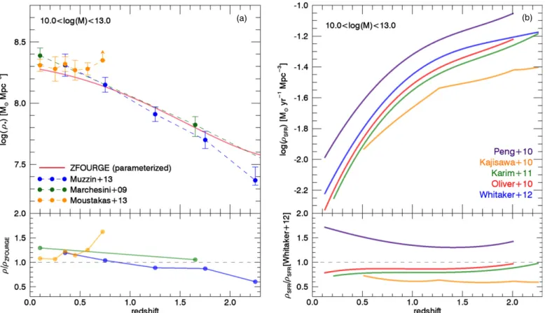
We first ask whether this disagreement is particular to the star formation rates measured in the Whitaker et al. (2012) star-forming sequence. We perform a comparison between the integrated star formation rate densities implied by star-forming sequences from the literature, shown in Figure7 (Oliver et al.
(a) (b)
Figure 7.Panel (a) shows the buildup of stellar mass density in the range 10<log(M/M)<13 as measured from multiple stellar mass functions. Below, the ratio of the measured stellar mass density relative to ZFOURGE is shown. The buildup of stellar mass varies between observations by a factor of about two, and ZFOURGE is comparable to other stellar mass functions in this respect, although it does measure a higher mass density in low-mass galaxies. In panel (b), we show the global star formation rate in galaxies with 10<log(M/M)<13 as calculated from different observed star-forming sequences. Below, we show the ratio of the measured global star formation rate relative to that implied by the Whitaker et al. (2012) star-forming sequence. The global star formation rates also vary by a factor of∼2, and the Whitaker et al. (2012) star-forming sequence is comparable to other observed star-forming sequences.
2011; Whitaker et al. 2012). We use the abundance of star-forming galaxies from ZFOURGE to convert the star-star-forming sequence into star formation rate densities. The implied, global star formation rates vary by a factor of two but display sim-ilar redshift evolution. The simsim-ilar redshift evolution between studies is due to the broad agreement in the redshift evolution of the normalization of the star-forming sequence. The actual offsets are due to a combination of different normalizations and different slopes; crucially, changing the limits of integra-tion has a significant effect on this comparison because of the difference in observed slopes. These differences in slopes and normalization may come about due to different SFR indica-tors, different adopted conversions from luminosity to SFR, different dust corrections, selection effects, or different def-initions of a star-forming galaxy (Speagle et al. 2014). Be-cause the redshift evolution differs little between studies, the relative rate of change may be well constrained, at least for galaxies with log(M/M)>10. Notably, the∼0.3 dex study-to-study variation between star formation rates is comparable in size to the systematic decrease in star formation rates necessary to bring the evolution of stellar mass and star formation rates into agreement.
Because many of the observable SFR indicators are primarily driven by radiation from massive stars, one way to decrease the observed star formation rates is to postulate a top-heavy IMF (e.g., van Dokkum2008). It has been claimed in the past that a top-heavy IMF is necessary to reproduce the properties of the submillimeter galaxy population (Baugh et al.2005; Dav´e et al.
2010), though recent studies may have resolved this tension
(Hayward et al.2013). There is not enough systematic evidence so far for a top-heavy IMF to be compelling (Bastian et al.2010). Alternatively, systematic overestimation of stellar masses at high redshift could solve the tension with star formation rates. The cumulative redshift-dependent errors in the mass function necessary to be consistent with the modified star-forming sequence can be read directly from the bottom panels of Figure3: the error at high masses would have to be 0.2–0.3 dex and 0.4 dex at low masses. At the high-mass end, errors could potentially come from systematic errors in fitting the light profile (Bernardi et al. 2013). At the low-mass end, stellar masses may be significantly overestimated because of emission-line contributions to the observed flux. Fixing the stellar metallicity to the solar value is likely a poor approximation at high redshift and may lower stellar mass estimates as well, particularly at the low-mass end (Mitchell et al.2013). It is also possible that the exponentially decaying star formation histories (SFHs) are poor fits to the true SFHs ofz=2 galaxies, which would decrease the stellar mass at all masses (Papovich et al.2011).
In Figure7, we compare the integrated stellar mass density from the ZFOURGE survey to other results from the literature (Marchesini et al.2009; Muzzin et al. 2013; Moustakas et al.
(a) (b) (c)
Figure 8.Contribution to the global star formation rate density as a function of galaxy stellar mass. This is calculated by multiplying the abundance of star-forming galaxies in ZFOURGE by the star-forming main sequence. Incompleteness in the observed star-forming sequence from Whitaker et al. (2012) is indicated by the dashed line. Extrapolating the observed star-forming sequence results in a substantial contribution from low-mass galaxies to the star formation rate density, particularly at high redshift.
of the relatively high abundance of low-mass galaxies at high redshift in ZFOURGE.
This comparison shows that the uncertainties in the absolute value of stellar mass density in the literature are at least a factor of two, and this difference is redshift dependent. These systematic redshift-dependent errors in stellar mass estimates may substantially contribute to the difference between the growth of stellar mass and the star formation rate atz=2.
We note that altering the IMF for low-mass stars as suggested by Conroy & van Dokkum (2012) will affect star formation rates and stellar masses equally and thus will not solve the tension between them.
4.3. Which Galaxies Dominate the Cosmic Star Formation Rate Density?
Here we examine the effects of different forms of the star-forming sequence on the global star formation rate. The mass-dependent contribution to the global star formation rate implied by the star-forming sequence, calculated viansf×SFR(M), is shown in Figure8.
With no modifications to the low-mass slope of the star-forming sequence, low-mass galaxies dominate the cosmic star formation rate atz=2 and continue to contribute substantially to the cosmic star formation rate at lower redshifts. This is consistent with Reddy & Steidel (2009), which suggests that sub-L∗ galaxies constitute up to 93% of the unobscured UV cosmic star formation rate density at 2 < z < 3. However, Sobral et al. (2014) use data from a narrow-band survey of Hα
emission atz=2.23 to argue that the contribution to the cosmic star formation density peaks at galaxies of 1010M
. This is in agreement with thez∼1 star formation rate density measured from the ROLES survey (Gilbank et al.2010). Semianalytical models predict a peak at a similar location, though at slightly higher stellar masses:∼1010.5M
, decreasing to 1010M at
z=0 (Lagos et al.2014).
Adopting a steep low-mass slope, as suggested by our analysis, substantially decreases the implied contribution from low-mass galaxies, in agreement with Gilbank et al. (2010) and Sobral et al. (2014), though notably the Gilbank et al. (2010) star formation rate density falls off more sharply toward
low stellar mass because of differences between the ROLES and ZFOURGE stellar mass functions (Gilbank et al. 2011). The peak of the cosmic star formation rate density depends on the exact location of the transition between high-mass slope and low-mass slope; in our model, this is fixed to 1010.5M. The star formation rates implied by the evolution of the stellar mass function have an almost identical shape to the modified low-mass star-forming sequence, but with a ∼0.3 dex normalization offset atz=2. Both of the modified star-forming sequences presented in our study indicate that the contribution to the cosmic star formation peaks in galaxies of 1010–1010.8 solar masses. An interesting parallel can be drawn with the star formation efficiency (defined asM∗/Mhalo). Hydrodynamical simulations and abundance-matching models indicate that the star formation efficiency peaks at a similar stellar mass log(M/M)=10.0–10.3 for 0< z <4 (Behroozi et al.2013b; Genel et al.2014).
4.4. Comparison to Galaxy Formation Models
The observed star formation rates of galaxies atz=1–3 have long been in tension with theoretical expectations, which include semianalytical, hydrodynamical, and semiempirical models of galaxy formation (Bouch´e et al.2010; Firmani et al.2010; Dav´e et al.2011; Lilly et al.2013; Dekel & Burkert2014; Genel et al.
2014; Mitchell et al. 2014). In models of galaxy formation, the specific star formation rate of galaxies roughly tracks the specific dark-matter accretion rate (Weinmann et al.2012; Lilly et al.2013; Mitchell et al.2014; Genel et al.2014; Peng et al.
2014) with a normalization offset of∼3, required to match low-redshift observations (Genel et al. 2014). However, between
Figure 9.Star-forming sequences from semianalytical models (Guo et al.2013b; Mitchell et al.2014), abundance-matching models (Behroozi & Silk2014, shown only in the middle panel), and hydrodynamical models (Genel et al.
2014) also show a steep low-mass slope and a shallow high-mass slope. This may be a universal feature of models that reproduce the cosmic evolution of the stellar mass function.
9.27 < log(M/M) < 9.77 occurred much more recently than in the models. Mitchell et al. (2014) advocate for a similar picture, arguing that the steep star-forming sequence in semianalytical models must be adjusted at low stellar masses to match observations of a shallower slope.
In Figure9, we compare the star-forming sequence in semi-analytical models (Guo et al. 2013a; Mitchell et al. 2014), stellar mass–halo mass abundance-matching (SHAM) model (Behroozi & Silk2014), and hydrodynamical models (Genel et al.2014) to the star-forming sequence we derive from the ZFOURGE mass functions. They are strikingly similar in shape, with a slope of∼0.6 at the high-mass end and a slope of∼1 at the low-mass end. Considering that semianalytical, hydrody-namical, and abundance-matching models must necessarily be consistent with the evolution of the stellar mass function, it is
perhaps not surprising that they show behavior similar to the star formation rates derived from the observed redshift evolution of the stellar mass function.
We suggest that a mass-dependent slope for the star-forming sequence would ease the discrepancy between models and observations. A steep low-mass slope at z > 1 is not ruled out by current studies: see the discussion in Section 3.2.1. Adopting a star-forming sequence with a slope close to unity at low masses means that low-mass galaxies grow in a self-similar fashion, implying thatM/M˙ =c(z), wherec(z) is a constant that depends only on redshift. Thus, the relative growth of low-mass galaxies would be independent of low-mass but still dependent on redshift. The star formation rate of low-mass galaxies will then scale similarly to the specific dark-matter accretion rate, which, forM˙ ∝Mα, hasα=1.1 (Neistein & Dekel2008).
4.5. Alternatives to Changing the Low-mass Slope: Undetected Quiescent Galaxies and Mergers
Enforcing a steep slope in the star-forming sequence at low stellar masses is one way to construct a consistent picture of the buildup of stellar mass. However, it is important to explore possible alternative explanations as well: namely, the merger rate and the possibility of a hidden population of quiescent galaxies. Higher merger rates will remove low-mass galaxies before they grow rapidly, and large populations of quiescent galaxies will decrease the average star formation rate as a function of mass.
We calculate the merger rate needed to produce a single-slope star-forming sequence. This is derived by growing the stellar mass function with the single-slope star-forming sequence, then computing the difference between the observed mass function and the mass function grown by star formation. This difference, divided by the time step, is the required rate of destruction by mergers. Note that while we neglect the galaxy growth due to mergers in this procedure, in practice, the growth rate due to mergers in our model is negligible for galaxies with stellar mass lower than 1011M.
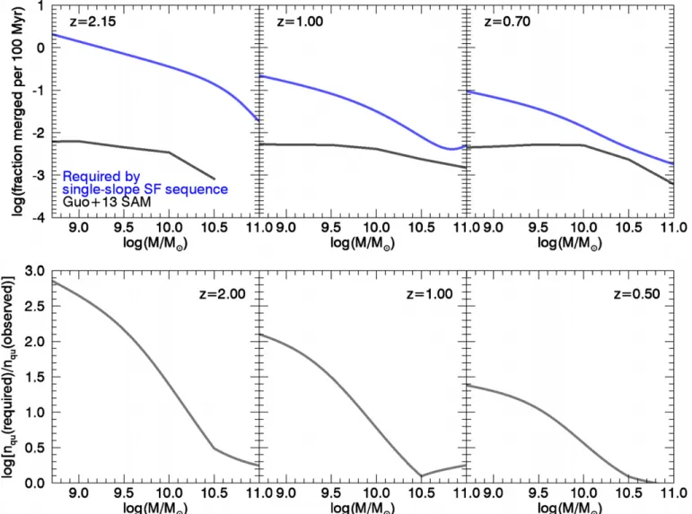
The same effect can be caused by undetected quiescent galaxies. To calculate the required number density of undetected quiescent galaxies, we first calculate the growth of the stellar mass function in a single time step due to the single-slope star-forming sequence from Whitaker et al. (2012). Then, we compare this growth rate to the growth rate in a single time step required to match the observed stellar mass function. The increase in the number of quiescent galaxies necessary to reconcile these two growth rates is inferred from Equation6. Figure10shows the merger rate necessary for the observed star-forming sequence to be consistent with the evolution of the mass function. We compare this directly to the merger rate from the Guo et al. (2013b) semianalytical model. Atz=2, merger rates would have to be over two orders of magnitude higher than expected in order to be consistent with the observed star-forming sequence. This difference decreases with redshift, but even atz=0.5 it is necessary to increase the rate of low-mass mergers by an order of magnitude to match the growth of the mass function.
Figure10also shows the factor by which the number density of quiescent galaxies would have to increase to bring star formation rates and the growth of stellar mass into agreement. The number density of quiescent galaxies at log(M/M)=9 would have to increase by almost three orders of magnitude at
Figure 10.Top panels: the merger rate required for a low-mass extrapolation of the star-forming sequence to be consistent with the evolution of the mass function. This is compared to the mass-dependent destruction rate of galaxies from the Guo et al. (2013b) SAM. A mass-independent slope for the star-forming sequence implies merger rates that are orders of magnitude higher than predicted by dark-matter models, particularly atz=2. Bottom panels: the factor by which the observed number density of quiescent galaxies must increase to make a low-mass extrapolation of the star-forming sequence consistent with the evolution of the mass function. At low masses and high redshifts, the number density of quiescent galaxies would have to be three orders of magnitude higher than what is observed. For reference, the quiescent mass function in ZFOURGE is complete to log(M/M)=9 atz=2.
ZFOURGE is estimated to be mass-complete for quiescent galaxies down to log(M/M) = 9 at z = 2.25. However, the ZFOURGE stellar mass-complete limit is estimated by comparing the magnitude of a single stellar population formed atz=5 to the magnitude limit of the survey. This calculation does not take into account the confounding effects of dust. If low-mass quiescent galaxies have a significant amount of dust at higher redshift, this would imply that the nominal mass-completeness of the survey is overestimated.
We conclude that while it is possible that a combination of merger rates and missing quiescent galaxies may be a factor in easing the tension between star formation rates and the growth of stellar mass, they are unlikely to be a dominant factor. The most likely solution remains a modification of the low-mass slope of the star-forming sequence.
4.6. Model Approximations
4.6.1. Scatter in Star Formation Rates
We model the growth of the stellar mass function by assuming all galaxies grow at the same rate. At fixed stellar mass, however,
galaxies are a diverse population and display a variety of star formation rates (van Dokkum et al.2011). It is thus important to discuss whether the assumption of a single growth rate at fixed mass is a valid one.
It is possible to mathematically prove that scatter in star formation rates does not influence the evolution of the mass function and that the only relevant parameter is the average star formation rate as a function of mass and time. Here, we sketch this proof briefly; the full proof will be presented in M. Franx et al. (in preparation).
The evolution of the mass function due to star formation is given by the following equation:
∂ψ(M, t)
∂t = − ∂ ∂M
ψ(M, t)M˙, (10)
this case, the massMis the x position, and the star formation rate is the velocity.
As further discussed by M. Franx et al. (in preparation), the consequence is that the evolution of the mass function due to star formation at anyM is determined byM˙ only and is the same for all models with a given ψ(M) and M˙. Hence the scatter in the star formation at a givenM does not influence the evolution of the mass function, as long asM˙ is given. It is not important on what timescale galaxies may move below or above the average. As shown by M. Franx et al. (in preparation), another way to see this quickly is by assuming that scatter is caused by two populations of galaxies with two different star formation rates. In AppendixB, we show that a sum of the two populations will satisfy the continuity equation, just like the two populations separately. This argument can be extended to an arbitrary number of subpopulations.
Thus, any galaxy population for which the mean star forma-tion rate as a funcforma-tion of mass is identical will evolve in the same fashion. The actual distribution of star formation rates does not affect the evolution of the stellar mass function: as long as the mean star formation rate as a function of mass is identical in any given distribution atevery time step, the mass function will evolve in an identical fashion.
4.6.2. Modeling Mass Loss from Galaxies
We adopt an instantaneous stellar mass loss model. In reality, the mass-loss rate of galaxies is time dependent, with the majority of it occurring in the first hundred million years. The efficiency of the instantaneous approximation will thus scale inversely with the specific star formation rate of galaxies, meaning that low-mass galaxies at high redshift are most affected by this approximation.
Stellar mass functions are tabulated using the current masses in stars and stellar remnants, thus implicitly taking this effect into account. To account for this in our model, the fraction of mass returned to the interstellar medium,R, would have to be modeled as SFH dependent. This would likely elevate the implied star formation rates at low masses by∼20%. This is not a dominant effect but would contribute toward reconciling stellar mass growth and star formation rates at high redshift and low masses.
5. CONCLUSION
In this study, we have examined the connection between the observed star-forming sequence and the observed redshift evo-lution of the stellar mass function. We have constructed a smooth parameterization of the growth of the stellar mass function from ZFOURGE and SDSS–GALEXdata and compared this growth to the growth implied by the observed star-forming sequence. We find that a simple extrapolation of the observed slope to low stellar masses is inconsistent with the observed evolution of the mass function. We conclude from this comparison that one or all of the following must be true: (1) the star-forming sequence steepens at low masses, (2) the destruction rate of low-mass galaxies by mergers is very high, or (3) there is a dominant population of low-mass quiescent galaxies missing from high-redshift surveys. We use merger rates from semiana-lytical models to show that the merger rate of low-mass galaxies is several orders of magnitude too low to solve the issue. We also show that there would have to be several orders of magnitude more quiescent galaxies than observed atz = 2 to solve the issue, which is unlikely to be true in the mass-complete regime
Figure 11. Mass-dependent destruction rates and growth rates, measured directly from the Guo et al. (2013b) SAM as a function of redshift. Atz∼2, low-mass galaxies are being rapidly destroyed, but this rate of destruction decreases as redshift decreases. The opposite trend is seen at higher masses, whereby the rate of destruction for higher-mass galaxies increases with decreasing redshift. The growth rate due to mergers is a smooth and continuous function of mass.
of stellar mass surveys. We thus conclude that, in order to de-crease the star formation rates for galaxies with mass∼109M
, the star-forming sequence must steepen at low masses. This conclusion is supported by the observations of Whitaker et al. (2014).
We show that a mass-dependent slope for the star-forming sequence makes the global star formation rate more consistent with the growth of stellar mass density. However, even with a steeper star-forming sequence, there is a discrepancy of ∼0.3 dex between the growth of stellar mass density and the global star formation rates at high redshift. Comparing different studies in the literature, we find that there is an interstudy difference of∼0.3 dex in both the implied global star formation rates and the growth of the stellar mass density, and the redshift evolution of these quantities can differ substantially between studies. It is thus unclear whether measurements of star formation rates, stellar masses, or both need to change in order to tell a consistent story.
(a) (b) (c)
(d) (e) (f)
Figure 12.Identical to Figure3, except the dashed curves in the lower three panels now represent mass functions modulated by the mass-dependent destruction rates and growth rates from the Guo et al. (2013b) SAM. These can be compared directly to the solid curves, which do not include the effects of mergers. The effects of mergers in these calculations are relatively small at low masses. The purple line represents the star-forming sequence required to make the evolution of the stellar mass function, modulated by the SAM merger rates, match the observed evolution of the stellar mass function. The three models presented previously in the main body of the paper are shown here with faded colors.
We thank the anonymous referee for insightful suggestions and attention to details, which have greatly improved the qual-ity of the paper. Support from NASA Grant NNX11AB08G is gratefully acknowledged. K.E.W. is supported by an appoint-ment to the NASA Postdoctoral Program at the Goddard Space Flight Center, administered by Oak Ridge Associated Universi-ties through a contract with NASA.
APPENDIX A
MASS-DEPENDENT MERGER RATES FROM SEMIANALYTICAL MODELS
Our fiducial model, presented in the main body of the paper, uses the destruction rate of galaxies from the Guo et al. (2013b) SAM and assumes that the resulting mass growth occurs in 1:10 ratio mergers. This approximation has the advantage of enforcing mass conservation within our model.
However, this approximation also introduces several issues. First, by simplifying all mergers into 1:10 mass ratio mergers, the mass growth rate of a galaxy of massMis determined only by the destruction rate at 0.1*M, modulated by the ratio of number densities. In particular, this underestimates the mass growth due to mergers in high-mass galaxies, which do not just accrete intermediate-mass galaxies but also accrete a significant fraction of low-mass galaxies. Second, galaxies below the mass cutoff of our simulation (106M
) also deposit stellar mass into more massive galaxies, but this is not reflected in our prescriptions.
To address these issues, we directly measure the mass growth of galaxies due to mergers in the Guo et al. (2013b) SAM and apply them to the stellar mass function. The destruction
rates and growth rates as a function of mass are shown in Figure11. The growth due to mergers is a smooth function of mass and decreases smoothly and slowly as redshift decreases. The destruction rate due to mergers increases with redshift at the low-mass end and decreases with redshift at the high-mass end, such that a destruction rate that is relatively flat with mass at
z=0.38 becomes a destruction rate that is quite steep with mass atz=2.33. We note that the Millenium-II simulation probes a relatively small volume, such that at the highest masses, there are only a few galaxies from which to measure merger growth rates. The accuracy of the growth and destruction rates at the highest masses are thus strongly limited by both Poisson noise and cosmic variance.
We interpolate between the measurements in Figure11and apply both directly to the growth of the mass function. The resulting growth of the mass function, when combined with the three parameterizations of the star-forming sequence described in Section 3.2, is shown by the dashed lines in Figure 12. The main difference as compared to our preferred model is the growth of galaxies with log(M/M)>11, which increases substantially when using the SAM growth rates. Lower-mass galaxies experience less growth due to mergers, but because their growth was already dominated by star formation, this has little effect on the evolution of the mass function.
Figure 13.Upper panel shows the redshift evolution of the normalization for the double power-law fits to the star-forming sequence, and the lower panel shows the same for the low-mass slopes (solid line) and high-mass slopes (dashed line). The red line is the star-forming sequence derived from the mass function as described in Section3.2.3, and the purple line is done in the same way but after applying the SAM-measured merger rates. The slope of the star-forming sequence becomes an even stronger function of mass after including mergers.
sequence, but we now perform this fitafterincluding the effects of mergers. This star-forming sequence is shown in purple in Figure12. Note that it is not a functional fit that is shown (as is true for the star formation rates derived from the mass function without mergers), but the actual inferred star formation rates.
Including the mergers when fitting for the star-forming sequence slightly increases the star formation rates at low masses, while decreasing them substantially at high masses. This is because the main effect of mergers at low mass is the destruction of galaxies, while the main effect of mergers at high mass is additional mass growth. In fact, applying the Guo et al. (2013b) SAM merger growth rates to the high-mass end is more than sufficient to model the growth of high-mass galaxies in the ZFOURGE mass function: presumably, the merger growth rates in the real universe are lower than those measured from the SAM.
We also fit the merger-modulated star formation rates with a double power law with the same form as Equation (9). The redshift evolution of the normalization and the slopes is shown in Figure 13. Crucially, the evidence for a mass-dependent slope is not altered by including the growth rate due to mergers. In fact, this conclusion is strengthened, though this highlights an important point: deriving the high-mass slope
of the star-forming sequence is very sensitive to the merger rate (conversely, the low-mass slope is very stable to the merger rate). However, using merger growth rates measured directly from the SAM violates mass conservation. Specifically, the Guo et al. (2013b) mass functions have a higher number density of low-mass galaxies than is observed in ZFOURGE, which means that for the same rate of destruction of galaxies, the merger growth rates from the semianalytical model will be higher than the simple 1:10 merger growth rates assumed in our model. This results in a mass growth at the high-mass end that is more than enough to explain the growth of the mass function. This extra growth is reflected in the high-mass drop-off in the merger-modulated star formation rates from the stellar mass functions, visible in Figure12.
APPENDIX B
LINEARITY OF THE CONTINUITY EQUATION
In this section, we prove that Equation (10) presented in the text is linear and thus can be generalized to the entire galaxy population.
First, assume that we have two populations of galaxies, each with a different dependence of star formation rate on stellar mass. The continuity equation for each individual population is
∂ψi(M, t) ∂t = −
∂
∂M[ψi(M, t) ˙Mi ],
where the subscriptiis either 1 or 2 for the two populations. We sum both sides of the continuity equation, as defined for galaxy populations 1 and 2. For the sum of the left-hand terms, we obtain
∂ψ1(M, t)
∂t +
∂ψ2(M, t)
∂t =
∂[ψ1(M, t) +ψ2(M, t)]
∂t
and for sum of the right-hand terms, we obtain
− ∂
∂M[ψ1(M, t) ˙M1 ]− ∂
∂M[ψ2(M, t) ˙M2 ]=
− ∂
∂M[ψ1(M, t) ˙M1 +ψ2(M, t) ˙M2 ].
Now, define ˙Mi to be the average star formation rate of the
combined galaxy population andψtot(M, t) to be the total mass function:
ψtot(M, t)=ψ1(M, t) +ψ2(M, t)
˙Mtot = ψ1(M, t) ˙M1 +ψ2(M, t) ˙M2 ψtot(M, t) .
Substitute these into the left- and right-hand sums, and we recover the original equation:
∂ψtot(M, t)
∂t = − ∂
∂M[ψtot(M, t) ˙Mtot ].
Thus, the continuity equation for the evolution of the galaxy population is linear.
REFERENCES
Abazajian, K. N., Adelman-McCarthy, J. K., Ag¨ueros, M. A., et al. 2009,ApJS,
182, 543
Baldry, I. K., Glazebrook, K., & Driver, S. P. 2008,MNRAS,388, 945