Independent Component Analysis on Spectral Domain
by Seonjoo Lee
A dissertation submitted to the faculty of the University of North Carolina at Chapel Hill in partial fulfillment of the requirements for the degree of Doctor of Philosophy in the Department of Statistics and Operations Research.
Chapel Hill 2011
Approved by:
Young K. Truong, Advisor
Haipeng Shen, Advisor
Richard L. Smith, Committee Member
J. S. Marron, Committee Member
c 2011 Seonjoo Lee
ABSTRACT
SEONJOO LEE: Independent Component Analysis on Spectral Domain. (Under the direction of Young K. Truong and Haipeng Shen.)
Independent component analysis (ICA) is an effective data-driven method for blind source
separation. It has been successfully applied to separate source signals of interest from their
mixtures. Most existing ICA procedures are carried out by relying solely on the estimation
of the marginal density functions, either parametrically or nonparametrically. In many
ap-plications, correlation structures within each source also play an important role besides the
marginal distributions. One important example is functional magnetic resonance imaging
(fMRI) analysis where the brain-function-related signals are temporally correlated.
In this thesis, we propose two novel ICA algorithms that fully exploit the correlation
structures within the source signals through spectral density estimation. Our methodology
development is two-fold: 1) ICA for auto-correlated sources via parametric spectral density
estimation (cICA-YW); 2) ICA for sources with mixed spectra via nonparametric spectral
density estimation and atom detection (cICA-LSP).
The cICA-YW focuses on the sources with autocorrelation and is implemented using
spectral density functions from frequently used time series models such as autoregressive
moving average (ARMA) processes. The time series parameters and the mixing matrix are
estimated via maximizing the Whittle likelihood function. We illustrate the performance of
the proposed method through extensive simulation studies and a real fMRI application. The
numerical results indicate that our approach outperforms several popular methods including
the most widely used fastICA algorithm. We also establish the sampling properties of the
proposed method.
For the cICA-LSP, we consider the case of sources with possibly mixed specta, where
ARMA estimates are often unstable. Specifically, we propose to estimate the spectral density
respectively. The mixed spectra and the mixing matrix are estimated via maximizing the
Whittle likelihood function. We illustrate the performance of the proposed method through
Keywords: blind source separation, independent component analysis, discrete fourier
trans-form, temporally correlated time series, harmonic functions, functional magnetic resonance
Table of Contents
List of Figures . . . ix
1 Introduction . . . 1
1.1 Independent Component Analysis . . . 1
1.2 Application of ICA in Biomedical Imaging Data . . . 4
2 ICA for Autocorrelated Sources: cICA-YW . . . 8
2.1 Introduction . . . 8
2.2 Colored Independent Component Analysis . . . 10
2.2.1 Preliminaries . . . 10
2.2.2 The Whittle Likelihood . . . 11
2.2.3 ICA for AR Sources and Its Algorithm . . . 13
2.2.4 ICA for White Noise Sources . . . 16
2.2.5 Extension to general ARMA Processes . . . 17
2.3 Simulation Studies . . . 18
2.3.1 Blind Separation of Colored Sources . . . 18
2.3.2 Blind Separation of White Sources . . . 20
2.3.3 Detection of Activated Brain Regions . . . 22
2.4 Application to Real fMRI Data . . . 29
2.4.1 Data Description . . . 29
2.4.2 Analysis . . . 29
2.4.3 Results . . . 30
2.5 Conclusion . . . 33
3 Asymptotics of cICA-YW . . . 36
3.1 Introduction . . . 36
3.2.2 Discrete Fourier Transforms and the Periodograms . . . 38
3.2.3 Parametric Spectral Density Estimation . . . 39
3.3 Main Results . . . 40
3.3.1 Prewhitened cICA . . . 44
3.4 Simulation Study . . . 46
3.5 Proof of Theorems . . . 49
3.5.1 Preliminary . . . 49
3.5.2 Proof of cICA . . . 52
4 Nonparametric ICA with Logspline Spectral Density Estimation . . . 62
4.1 Logspline Spectral Density Estimation . . . 62
4.2 Prewhitened cICA via Nonparametric Spectral Density Estimation . . . 66
4.2.1 The Whittle Likelihood . . . 66
4.2.2 Algorithm . . . 68
4.3 Simulation Studies . . . 71
4.3.1 Sources with mixed spectra-Fourier frequency atoms . . . 71
4.3.2 Sources with mixed spectra-Non-Fourier frequency . . . 74
4.4 Future Work . . . 78
5 Appendix . . . 83
5.1 Additional Simulation for cICA-YW . . . 83
5.2 Proof of Theorems in Chapter 3 . . . 88
5.3 Proofs of Lemmas . . . 88
5.4 Statement of Result of wICA . . . 99
5.4.1 White Noise Sources . . . 99
5.5 Proofs of wICA . . . 102
5.5.1 Preliminary . . . 102
5.5.2 Proofs of wICA . . . 104
5.6 Covariances of Score Functions . . . 111
5.6.2 Covariances of Score Functions for cICA . . . 112
5.7 Hassian Matrix . . . 114
5.7.1 wICA . . . 114
5.7.2 cICA . . . 115
List of Figures
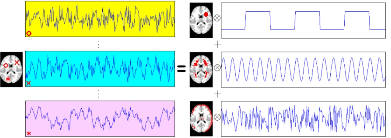
1.1 ICA Illustration in fMRI Studies . . . 5
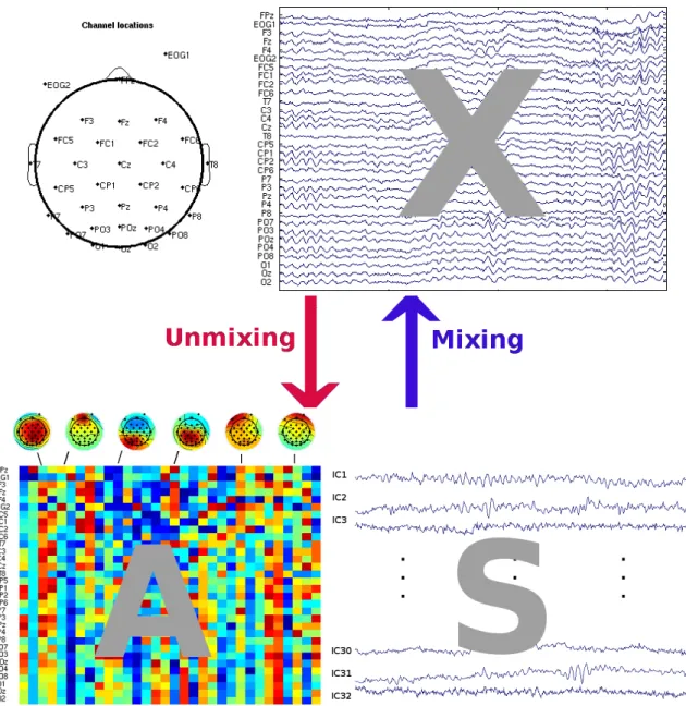
1.2 ICA illustration in EEG studies . . . 6
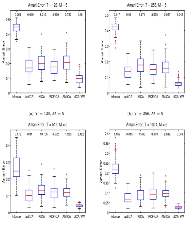
2.1 Performance Comparison for ARMA Sources . . . 19
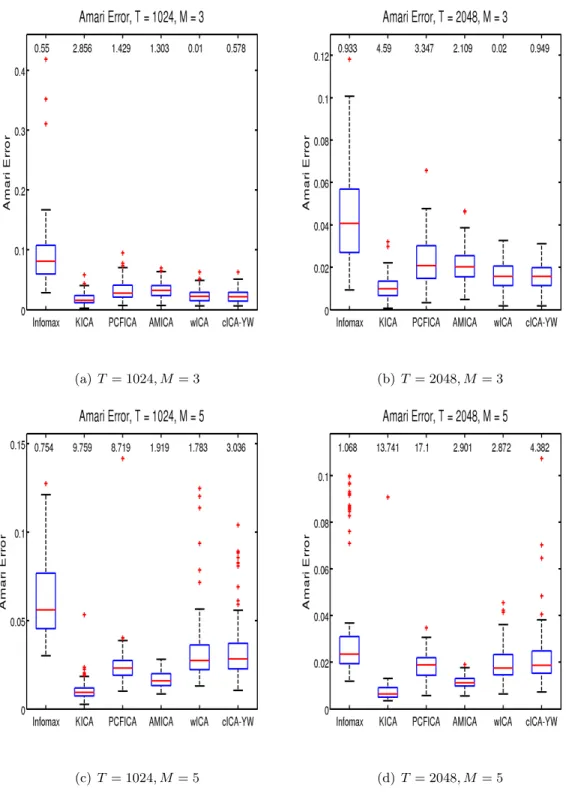
2.2 Performance Comparison for White Noise Sources . . . 21
2.3 Task function with noise at different SNRs . . . 23
2.4 The True Independent Components and Spatial Maps . . . 25
2.5 Comparisons of False Positive and False Negative Rates . . . 27
2.6 Block Design: Spatial Maps under SNR=1 . . . 28
2.7 Experimental Paradigm . . . 30
2.8 Real fMRI Analysis Results . . . 34
2.9 Real fMRI Analysis Results . . . 35
3.1 Performance Comparison for Nonorthogonal Matrix . . . 47
3.2 Order Selection Comparison between AIC and BIC . . . 48
3.3 Spectral Density Estimation with BIC order selection atT = 1024 . . . 50
4.1 Performance comparison . . . 73
4.2 Simulation Study I: Performance comparison . . . 73
4.3 Order Estimation . . . 74
4.4 Comparison of the estimated spectra . . . 75
4.5 Atom detection for the estimated sources . . . 76
4.6 Performance comparison for sources with mixed spectra . . . 77
4.7 Performance comparison for sources with mixed spectra . . . 78
4.8 Comparison of the estimated spectra of the sources . . . 79
4.9 Order Estimation of cICA-YW . . . 80
4.11 Atom Detection Rates at Each Frequencies. . . 81
5.1 Block Design: Spatial Maps under SNR=0.5 . . . 84
5.2 Block Design: Spatial Maps under SNR=1 . . . 85
5.3 Block Design: Spatial Maps under SNR=2 . . . 86
5.4 Block Design: Spatial Maps under SNR=4 . . . 87
5.5 Simulation Study IV: The True Independent Components . . . 88
5.6 Simulation Study IV: False Positive and Negative Rates at Different SNRs . . 89
5.7 Event Related Design: Spatial Maps under SNR=0.5 . . . 90
5.8 Event Related Design: Spatial Maps under SNR=1 . . . 91
5.9 Event Related Design: Spatial Maps under SNR=2 . . . 92
Chapter 1
Introduction
1.1
Independent Component Analysis
Independent component analysis(ICA) is an effective data-driven technique for extracting the
hidden source signals from mixtures of the observed signals, which is also known as theblind
source signal (BSS) problem in digital signal or image processing literature. It has many
important applications in acoustic signal processing (Hyv¨arinen et al., 2001); finance (Back
and Weigend, 1997); biomedical image analysis such as functional magnetic resonance imaging
(fMRI) (McKeown et al., 2003; Calhoun et al., 2009), electroencephalography (EEG), and
magnetoencephalography (MEG) (Makeig and Onton, 2009); system monitoring (Ge and
Song, 2007; Fiori and Burrascano, 2001). More extensive literature review can be found
in Stone (2004); Hastie et al. (2009); Cichocki et al. (2009); Comon and Jutten (2010).
The ICA problem can be formally expressed as follows. Suppose there areM mixed signals
of length T each, which are stored in the observed signal matrix X. ICA then allows one to
decomposeX as
XM×T =AM×MSM×T, (1.1.1)
whereAis a non-random mixing matrix andSis a matrix ofindependent source signals. The
goal of ICA is to recover the latent source signals (rows ofS) as
Many ICA procedures have been developed over the last fifteen years. A majority of the
methods are instantaneous mixtures, which are based on estimates of the marginal densities
of the sources, either parametrically or nonparametrically. Parametric approaches include
infomax(Bell and Sejnowski, 1995; Lee et al., 1999), which estimates the density parameters
via minimization of mutual information, and is equivalent to maximum likelihood estimation
using high-order cumulants (Comon, 1994);JADE(Cardoso and Souloumiac, 1993), which is
based on high-order cumulant and joint diagonalization; orfastICA(Hyv¨arinen et al., 2001)
that maximizes non-Gaussianity as measured by the approximated negative-entropy.
Parametric approaches sometimes can be too rigid. More flexible nonparametric methods
include estimating the score function using kernel approximation (Vlassis and Motomura,
2001), kernel density estimation (Bach and Jordan, 2003; Boscolo et al., 2004; Chen and
Bickel, 2005; Shen et al., 2006; Chen, 2006), smoothing splines (Hastie and Tibshirani, 2003),
B-spline approximation (Chen and Bickel, 2006), and logsplines (Kawaguchi and Truong,
2009). Two other relaxations of the basic ICA model are subspace ICA (Hyv¨arinen and
Hoyer, 2000; Sharma and Paliwal, 2006) that allows the sources to form mutually independent
subgroups and does not require the sources within the same subgroup to be independent; and
AMICA (Palmer et al., 2008) that uses mixtures of Gaussian scale mixtures to model the
sources, which was extended to include mixtures of linear processes (Palmer et al., 2010).
Note that when all the sources are mutually independent, subspace ICA reduces to ordinary
ICA (Hyv¨arinen and Hoyer, 2000).
All the above methods, however, only make use of the marginal densities (with the
ex-ception of the recent extention of AMICA), which do not contain information about the
correlation structures within the source signals. For example, in fMRI studies the
experiment-stimulus related signals or physiological signals such as heart beat or breathing are usually
periodic, and therefore embedded in the fMRI data are some autocorrelation or colored noise
structures within the signals (Bullmore et al., 2001). Such information is not incorporated
when using the marginal-density-based ICA methods. In this thesis we develop ICA
ap-proaches that take into account the correlation structures within the sources. Our methods
financial time series. See Hyv¨arinen et al. (2001) for more details.
To the best of our knowledge, Pham and Garat (1997) is the first ICA procedure that
takes into account the autocorrelation structures within the sources. The authors imposed
certain parametric correlation assumptions on the sources. Specifically, they assumed that
the spectral density of each source was known up to some scale parameters, and proposed a
quasi-maximum likelihood method to recover the sources. Their formulation is in the spectral
domain, and builds upon the asymptotic independence and normality of discrete Fourier
Transform (DFT). Since the spectral densities are known except the scale parameters, the
authors used the corresponding (known) separating filters in the quasi-likelihood, and only
needed to maximize the likelihood to get estimates for the scale parameters and the mixing
matrix.
Although the spectral domain approach of Pham and Garat (1997) is natural and
in-novative, their assumption that the spectra of the sources are known can be unrealistic in
practice. In this thesis, we relax that assumption and propose a new spectral domain ICA
procedure for sources with autocorrelation, i.e. colored sources. In particular, our procedure
assumes certain parametric time series models for the source signals, and estimates the model
parameters through parametric spectral density estimation. (Note that our method covers
the special scenarios when the source signals are white or uncorrelated.) In addition, we
use the Newton-Raphson method to improve the optimization efficiency, and incorporate the
Lagrange multiplier method for orthogonal constraints.
On a related note, an earlier attempt to examine the source autocorrelation was described
by Pearlmutter and Parra (1997). They introduced the contextual ICA by considering
Xt= p X u=0
AuSt−u,
a multivariate version of the autoregressive process of order p: AR(p). The autocorrelation
is clearly specified by the convolution relationship. In fact, this formulation is also referred
to as convolutive ICA. See Dyrholm et al. (2007) for a very thorough survey of this topic.
wherep= 0. In practice, the AR order pwill be ideally small and one way to achieve this is
to model each sourceStby a moving-average process of order q: MA(q). The parameters are
estimated via the likelihood derived from the standard time-domain method in time series,
with logistic distribution as the baseline distribution. Dyrholm et al. (2007) suggested to use
Bayesian information criterion (BIC) to estimate the parametersp and q.
Our main contributions are two folds: (1) convolutive ICA for autocorrelated sources with
parametric spectral density estimation (cICA-YW); (2) convolutive ICA with nonparametric
spectral density estimation for the source with mixed spectra (cICA-LSP). The cICA-YW
is flexible for AR order selection for convolutive ICA, and its computational advantage has
been well documented in Lee et al. (2011). In addition, its sampling properties have been
investigated.
This dissertation is structured as follows. In Chapter 2, we provide details of the cICA-YW
procedure with an application to fMRI data. In Chapter 3, sampling properties of cICA-YW
are studied with order selection performance comparison. In Chapter 4, we provide details of
cICA-LSP with numerical studies.
1.2
Application of ICA in Biomedical Imaging Data
In this section, we introduce two popular applications of ICA, fMRI and EEG. An fMRI
dataset is four-dimensional consisting of a three-dimensional image (or a 3D volume) being
observed over time. Each 3D fMRI image consists of a certain number of two-dimensional
slices, and each slice is made up of individual cuboid elements called voxels. The data are
usually represented as a space-time matrix of dimension V ×T, where V is the number of voxels in one image andT is the number of time points in the experiment. Thus each column
of the matrix represents an fMRI image withV voxels and each row is the time course observed
at one specific voxel.
The recorded time series can be viewed as a mixture of source signals that are temporally
correlated, corresponding to the experimental stimuli, physiological functions such as heart
1.2. For simplicity, this toy example considers only one slice of the brain. The left side of
the figure plots the voxel time series (or the rows of the matrix) from three exemplary voxels
in this slice. Note that each voxel is marked using a different symbol that is matched with
its corresponding time series plot. The goal of ICA is to recover the (three) independent
temporal sources (the rows ofSin (1.1.1)), which are displayed on the right side of the figure,
and represent an experimental stimulus, cardiac or respiratory effect, and a movement effect,
respectively. The columns of the mixing matrixA in (1.1.1) are shown as the spatial maps,
where the voxels activated by the corresponding temporal signals are colored as red. Note
that typical fMRI data have a high spatial dimension (V ≈ 200,000), which is much larger than the number of extracted independent components (M = 3 in our example). Hence
dimension reduction is usually performed prior to ICA of fMRI data.
The applications of ICA to fMRI are classified into two categories based on their goals:
spatial ICA (sICA) and temporal ICA (tICA). The sICA looks for independent image
com-ponents (columns of A). The tICA, however, assumes independence of time courses (rows
of S). In both cases, we view a single image component (one column of A) as one spatially
distributed set of voxels that is induced by the corresponding time course in one row of S.
This dissertation focuses on temporal ICA.
Figure 1.1: Illustration of ICA in fMRI Studies. Simulated fMRI data (left) are modeled as the outer product of three spatial maps and their corresponding temporal components (right). The time series plots of three randomly selected voxels are depicted on the left side of the plot.
features such as EEG. EEG is the recording of changes of action potential along the scalp
produced by the firing of neurons within the brain. Action potential generation is provoked
by receipt of neuronal signal input within a brief time window. The emergence of
synchro-nized local fired potentials across a cortical area reflect changes in occurrence of joint spiking
events across groups of associated neurons in that area. The source potentials spread broadly
through the brain, skull and scalp and the mixing of these signals is observed at each scalp
electrode. The observed EEG signals arriving at different electrodes are the sum of brain
source activities;non-brain sources such as scalp muscle, eye movement, and cardiac artifacts;
and electrode and environmental noise. Figure 1.2 illustrates how ICA can be applied to EEG
data. In the upper panel, the EEG signals are collected from different electrodes along the
skull. ICA decompose the observed data (X) into the product of scalp map or mixing matrix
(A) and the independent source matrix (S). Each column of A gives the relative strengths
and polarities of projections of the corresponding component source signal to each of the scalp
channels. The values in the columns are color coded and interpolated onto heads to visualize
the topographic projection patterns associated with each of the sources. In other words, ICA
recovers a set of relevant independent components from EEG data through finding a spatial
Chapter 2
ICA for Autocorrelated Sources:
cICA-YW
2.1
Introduction
Independent component analysis (ICA) is an effective data-driven technique for extracting
the source signals from their mixtures (Hyv¨arinen et al., 2001; Stone, 2004). It aims to solve
the “blind source separation” problem by expressing a set of observed mixed signals as linear
combinations of independent latent random variables (or source signals or components). It
has many important applications, especially infunctional magnetic resonance imaging(fMRI)
analysis (McKeown et al., 2003; Stone, 2004; Huettel et al., 2008; Calhoun et al., 2009).
To the best of our knowledge, Pham and Garat (1997) is the first ICA procedure that
takes into account the autocorrelation structures within the sources. The authors imposed
certain parametric correlation assumptions on the sources. Specifically, they assumed that
the spectral density of each source was known up to some scale parameters, and proposed a
quasi-maximum likelihood method to recover the sources. Their formulation is in the spectral
domain, and builds upon the asymptotic independence and normality of discrete Fourier
Transform (DFT). Since the spectral densities are known except the scale parameters, the
authors used the corresponding (known) separating filters in the quasi-likelihood, and only
needed to maximize the likelihood to get estimates for the scale parameters and the mixing
Although the spectral domain approach of Pham and Garat (1997) is natural and
in-novative, their assumption that the spectra of the sources are known can be unrealistic in
practice. In this chapter, we relax that assumption and propose a new spectral domain ICA
procedure for sources with autocorrelation, i.e. colored sources. In particular, our procedure
assumes certain parametric time series models for the source signals, and estimates the model
parameters through parametric spectral density estimation. (Note that our method covers
the special scenarios when the source signals are white or uncorrelated.) In addition, we
use the Newton-Raphson method to improve the optimization efficiency, and incorporate the
Lagrange multiplier method for orthogonal constraints.
By contrast, our approach is to embed the autocorrelation into the sources via the
in-stantaneous ICA. For instance, if each source is modeled by an autoregressive model with the
same orderp, then our model yields the convolutive ICA described above. The choice of pfor
all sources is convenient for the comparison (with the convolutive ICA). We can in fact allow
each source to have a different AR order. Moreover, we can enhance the flexibility by fitting
an autoregressive and moving-average process of orderspandq (ARMA(p, q)) to each source.
The model parameters p and q can be of course source specific and can be estimated via an
information based method such as AIC or BIC. The autocorrelation related parameters or
the coefficients of the ARMA process are estimated using the Whittle likelihood, which is a
discrete Fourier transform (DFT) based method. Thus this is a distribution-free approach, see
Section 2.3 for a more detailed description of our method. Also an authoritative comparison
between the two likelihood approaches is documented in Dzhaparidze and Kotz (1986).
Estimating the mixing matrix has an important application in studying brain function
using fMRI through activity detection. Many statistical methods have been developed that
can be roughly classified into either hypothesis-driven or data-driven approaches. Hypothesis
driven approaches are based on conventional regression models to identify voxels whose time
series are significantly correlated with the experimental task(s). Examples include statistical
parametric mapping (Friston et al., 2007), a variety of Bayesian techniques implemented
in FSL (Woolrich et al., 2009), diagnosis procedures for noise detection (Zhu et al., 2009),
connecting the activated voxels for region-of-interest (ROI) analysis is something else to be
desired (Huettel et al., 2008). Alternatively, data-driven approaches for ROI analysis via
mixing matrix estimation include principal component analysis (PCA) (Viviani et al., 2005),
dynamic factor models (Park et al., 2009), clustering methods (Venkataraman et al., 2009),
and ICA (McKeown et al., 2003; Esposito et al., 2005; Calhoun et al., 2009; Sui et al., 2009).
Our approach takes these data-driven procedures a step further by exploiting the temporal
correlation structures while detecting the brain activation. It is therefore a temporal ICA
procedure.
The rest of the chapter is structured as follows. Section 2.2 describes our proposed method
for handling colored sources. We illustrate its performance and compare it against several
existing ICA methods through simulation studies in Section 2.3. The considered ICA methods
are also applied to analyze a real fMRI dataset in Section 2.4. We finally conclude the chapter
in Section 2.5.
2.2
Colored Independent Component Analysis
This section presents the details of our procedure for handling colored sources. We start with
some basic definitions in Section 2.2.1, followed by a discussion on the Whittle likelihood in
Section 2.2.2. For the purpose of easy understanding and presentation, we first describe the
procedure for autoregressive (AR) processes in Section 2.2.3. This is an important leading
case as Worsley et al. (2002) suggested that AR models are the most commonly used time
series approaches for the temporal correlation structure in fMRI analysis. We then discuss in
Section 2.2.4 how this procedure can be simplified to the special case of white noise processes,
and in Section 2.2.5 how it can be extended to general autoregressive moving average (ARMA)
processes.
2.2.1 Preliminaries
We start with several definitions in spectral analysis. Consider a vector-valued stationary
function cXX(u) = Cov(X(t),X(t+u)). If P∞u=−∞|cXX(u)| < ∞, we define the M ×M spectral density matrix of the series X(t) as
fXX(r) = 1 2π
∞
X u=−∞
cXX(u) exp{−iru}, r∈R,
where r is the angular frequency per unit time, or simply the frequency. The jth diagonal
element offXX,fXjXj, is the spectral density of the univariate time seriesXj(t). For a more
detailed discussion of spectral density, see Brillinger (2001).
In practice, we suppose that X(t),t= 0,1, . . . , T−1, are observed. Consider the Fourier frequencies rk = (2πk)/T,k= 0, . . . , T−1. Then, we can define the discrete Fourier transform
(DFT) of X(t),t= 0,1, . . . , T −1, as
ϕ(rk,X) = (ϕ(rk, X1), . . . , ϕ(rk, XM))>= T−1 X t=0
X(t) exp{−irkt},
and its second order periodogram as
˜f(rk,X) = 1
2πTϕ(rk,X)ϕ
∗
(rk,X),
whereϕ∗ is the conjugate transpose of the vectorϕ.
Considering the source signals S(t) = (S1(t), . . . , SM(t))>, t = 0,1, . . . , T −1, we can
similarly define their spectral density matrix fSS, DFT, and periodogram. Since the sources
are mutually independent, we have that fSS = diag{f11, . . . , fM M}, wherefjj is the spectral
density of thejth source.
2.2.2 The Whittle Likelihood
To minimize the bias in estimation associated with the misspecification of the time
se-ries distributions, Whittle (1952) formulated a likelihood approach by utilizing the
asymp-totic distributional properties of DFT (see Theorem 4.4.1 of Brillinger (2001)). Specifically,
suppose that we were able to observe the source signals and compute their periodograms:
can be shown that ˜f(rk, Sj) is asymptoticallyfjj(rk)χ22/2, independently of the other variates
fork = 0,1, . . . , T −1 and j = 1, . . . , M (see Theorem 5.2.6 of Brillinger (2001)). Thus the source log-likelihood is given by
L(fSS;S) =− 1 2
M X j=1
T−1 X k=0
(
˜f(rk, Sj) fjj(rk)
+ lnfjj(rk) )
, (2.2.1)
wherefSS is the diagonal matrix of the power spectra of the sources.
This is known as the Whittle likelihood in the literature and is being introduced to ICA
for the first time here. Asymptotic properties of the Whittle likelihood-based procedure
can be found in Dzhaparidze and Kotz (1986). Other than the desirable property that the
periodograms are independently distributed, one can see it is also advantageous that the
source autocorrelation can be examined through their power spectra. This forms the core of
our method.
Our next step is to express the above log-likelihood in terms of the periodograms computed
from the observed mixed signals. Using the mixing relationship (1.1.2) and the linearity of
DFT, the log-likelihood (2.2.1) can be rewritten as
L(W,fSS;X) =− 1 2
M X j=1
T−1 X k=0
(
e>j W˜f(rk,X)W>ej fjj(rk)
+ lnfjj(rk) )
+Tln|det(W)|,
(2.2.2)
whereej = (0,0, . . . ,0,1,0, . . . ,0)> with thejth entry being 1.
Once (2.2.2) is available, we maximize it to obtain the estimates of the unmixing
ma-trix W and the parameters in the power spectra of the sources (see Section 2.2.3). The
maximum Whittle likelihood approach can be interpreted as assigning a different weight of
(e>
jW)·(W>ej)
fjj(rk) to the source periodogram ˜f at the Fourier frequency rk. This procedure will
be referred to ascICAhereafter, wherec stands for color sources.
We make two remarks here. First, under this formulation, the novelty is the estimation
of the autocorrelations of the sources, which was not considered in Pham and Garat (1997);
the log-likelihood is subject to some identifiability constraints. ICA methods are known to
have permutation and scale ambiguity problems. Specifically, for a permutation matrix P
and a scalara, we haveX=W−1S=W−1(aP)(aP)−1S. To ensure the identifiability of W andS, we restrictW to be full rank matrix satisfying the following identifiability conditions
proposed by Chen and Bickel (2005):
1. max16k6MWjk = max16k6M|Wjk| for 1 6 j 6M, where Wjk is the (j, k)th entry of
W;
2. W1 ≺ · · · ≺ WM where Wj is the jth row of W. For ∀a,b∈ RM, we define a ≺ b
if there exists a k ∈ {1, . . . , M} such that the kth element of a is smaller than the corresponding element ofb, while all the elements before thekth entry are equal between
aand b. ( i.e. ak < bk and aj =bj, 16j6k−1, whereak is the kth element ofa.)
2.2.3 ICA for AR Sources and Its Algorithm
Penalized Whittle Likelihood
We first consider autoregressive (AR) models for the source signals, and assume that thejth
sourceSj follows a stationary AR(pj) process given by
Sj(t)− pj
X k=1
φj,kSj(t−k) =j(t), t= 0, . . . , T −1, j = 1, . . . , M,
where {φj,k} are the AR parameters and j(t) ∼ W N(0, σj2). The corresponding power
spectrum is given by
fjj(r) =
σ2j
2π|Φj(exp{−ir})|2
, r∈R,
where Φj(z) = 1−φj,1z− · · · −φj,pjz
pj is the corresponding AR polynomial.
Denoteφj = φj,1, . . . , φj,pj
>
The Whittle log-likelihood (2.2.2) can be rewritten as
L(W,φ,σ2;X) =−1
2
M X j=1
T−1 X k=0
(
2πe>j W˜f(rk,X)W>ej σ2
j/|Φj(exp{−irk})|2
+ ln σ
2 j/2π |Φj(exp{−irk})|2
)
+Tln|det(W)|.
(2.2.3)
If the data are prewhitened, the unmixing matrix W is orthogonal (Hyv¨arinen et al.,
2001). In this case, the Whittle likelihood can be further simplified by dropping the last term,
Tln|det(W)|. To incorporate the orthogonal constraints on the unmixing matrix, we propose to use Lagrange multiplier (Bertsekas, 1982). More specifically, we consider minimizing the
following penalized negative Whittle log-likelihood,
F(W,φ,σ2,λ) =−L(W,φ,σ2;X) +λ>C, (2.2.4)
whereλ= (λ1, . . . , λM(M+1)/2)> is the Lagrange parameter vector, and Cis a M(M+ 1)/
2-dimensional vector with the{(j−1)M+k}th element beingC(j−1)M+k= (WW>−IM)jk, j =
1, . . . , M, k = 1, . . . , j. Note that we need only M(M + 1)/2 constraints since the matrix
WW>−IM is symmetric.
We remark that there are other orthogonal constrained ICA algorithms based on
opti-mization over a set of all orthonormal matrices known as the Stiefel manifold. For instance,
see Edelman et al. (1998); Amari (1999); Douglas (2002); Plumbley (2004); Ye et al. (2006).
Iterative Estimation Algorithm
The minimization of the penalized criterion (2.2.4) is non-trivial. The computation involves
nonlinearly the M(M + 1)/2 elements of the unmixing matrix, as well as the AR model
parametersφand σ2, for a given set of the AR orders{pj}. In addition, the true AR orders also need to be estimated using model selection criteria. As such, our estimation algorithm
will be carried out in an iterative manner: alternating between updating the ICA unmixing
matrix and estimating the AR parameters (along with model selection) for a fixed unmixing
We start the iteration procedure with a certain set of the AR orders followed by
mini-mization of the criterion (2.2.4) in the following manner. First, start with an initial value of
f
W, then estimate φand σ2 by maximizing the un-penalized Whittle log-likelihood (2.2.3).
Alternatively, we can first recover the sources viaeS=WX, and then estimate the AR modelf
parameters φ using the Yule-Walker procedure (Brockwell and Davis, 1991). Our
experi-ence through numerical studies suggests that the two methods give similar results, while the
Yule-Walker procedure is computationally faster. Hence, in the remainder of the chapter, we
concentrate on the Yule-Walker procedure, and refer to the corresponding cICA procedure as
cICA-YW.
Once the AR coefficients φare estimated, we can estimate the variances σ2 using
˜
σj2(Wf,φ) =˜
2π T
T−1 X k=0
e>j Wf˜f(rk,X)Wf>ej|Φ˜j(exp{−irk})|2. (2.2.5)
Given the estimates ˜φand ˜σ2, we propose to obtain the updated estimate of the unmixing
matrixWby minimizing the penalized criterion (2.2.4). Since (2.2.4) is nonlinear with respect
toW, we use the Newton-Raphson method with Lagrange multiplier. To begin with, we find
the first and second derivatives of (2.2.4) with respect toWandλ, denoted as ˙F(W,λ;φ,σ2)
and H(W,λ;φ,σ2), respectively. Then we obtain the one-step Newton-Raphson update for
W and λas
c
W,λˆ
>
=
f
W,λ˜
>
−H(Wf,λ; ˜˜ φ,σ˜2) −1
˙
F(Wf,λ; ˜˜ φ,σ˜2). (2.2.6)
Finally, the above two steps are iterated to update (W,λ) and (φ,σ2) alternatingly until
convergence. To gauge the algorithm convergence, we use Amari error (Amari et al., 1996)
as the convergence criterion, which is defined as:
dAmari(W1,W2) =
1 M M X i=1 PM
j=1|aij|
maxj|aij| −1 ! + 1 M M X j=1 PM i=1|aij|
maxi|aij| −1
!
, (2.2.7)
W1W−21. This criterion has been used in the context of ICA (Bach and Jordan, 2003; Chen
and Bickel, 2005). When the Amari error betweenWc andWf is less than some threshold, the
iteration stops and we claim the algorithm converges. In our numerical studies the algorithm
usually converges within 30 iterations.
In practice, the true AR order of each source is not known and needs to be estimated.
We embed the order selection within the updating step for the AR model parameters, and
dynamically determine the suitable model for each iteration. In particular, we consider the
AR orderpjto vary between 0 and some threshold. We then select the “optimal” order using a
conventional model selection criterion such as the Akaike Information Criterion (AIC) (Akaike,
1974).
The complete iterative algorithm (with order selection) is summarized as follows:
The cICA-YW Algorithm
Initialize Wf,λ.˜
While the Amari error (2.2.7) is greater than the convergence threshold,
1. Estimate the sources by eS=WX. Forf j= 1, . . . , M,
(a) Estimate ˜φj using the Yule-Walker method with the order ˜pj selected by AIC.
(b) Compute ˜σ2j according to (2.2.5).
2. UpdateWf and ˜λ via the Newton-Raphson updating (2.2.6), using the estimates
˜
φand ˜σ2.
2.2.4 ICA for White Noise Sources
We now consider the case of white noise sources. Before proceeding, we remark that the
Whittle likelihood approach is essentially a second cumulant based method. Thus it will be
for ICA involving prewhitened data from a mixture of white noise sources. Therefore, we
focus on situations in which the dataset is an orthogonal mixture of white noise sources with
different variances. Now, since the mixing matrixAis orthogonal, it will not be necessary to
invoke the prewhitening step.
Suppose the jth white noise source has varianceσj2. Then its spectral density fjj equals
σj2/(2π). The Whittle log-likelihood is given by
L(W,σ2;X) =−1
2
M X j=1
T−1 X t=0
(
e>j W˜f(rk,X, T)W>ej σ2
j/(2π)
+ ln σj2/(2π)
)
. (2.2.8)
Note that if the sources are white noise, we apply the same weight to all the frequencies
when we maximize the Whittle log-likelihood (2.2.8). We also use the Lagrange multiplier
to ensure the identifiability of the unmixing matrix, and consider minimizing a penalized
negative Whittle log-likelihood similar to (2.2.4).
The estimation ofσ and W can be iterated as in cICA. There is no need to estimate the
AR coefficients nor select the AR order. We refer to this method aswICA. In Section 2.3.2
we show that with white noise sources, the wICA is very competitive with conventional ICA
methods; furthermore, the wICA and cICA perform similarly, which suggests that the model
selection step of cICA works well.
2.2.5 Extension to general ARMA Processes
The cICA procedure in Section 2.2.3 can also be extended to general ARMA processes in a
relatively straight-forward way.
Suppose the jth source follows some stationary ARMA(pj, qj) model so that
Φj(B)Sj(t) = Θj(B)j(t), j(t)∼W N(0, σj2),
whereB is the backshift operator, Φj(z) = 1−φj,1z− · · · −φj,pjz
pj, and Θ
j(z) = 1 +θj,1z+
· · ·+θj,qjz
given by
fjj(r) = σj2
2π
|Θj(e−ir)|2 |Φj(e−ir)|2
, r∈R.
We can update the Whittle log-likelihood (2.2.3) with the above power spectrum. The
iterative cICA algorithm of Section 2.2.3 can still be used to estimate the parameters, except
that special care is needed when estimating the time series model parameters and selecting
the AR/MA orders of the model. For the sake of saving space, we omit the details of the
technical derivation, and refer the readers to Brockwell and Davis (1991). We consider general
ARMA processes in the simulation studies of Section 2.3.
2.3
Simulation Studies
2.3.1 Blind Separation of Colored Sources
According to the ICA model (1.1.1), we first generated the source matrixS and theM×M
mixing matrixAseperately. We consideredM = 5 and simulated five independent stationary
ARMA time series under four different sample sizes (T = 128, 256, 512, 1024). The five
sources were generated as
• S1: AR(2),φ1 = 1, φ2 =−0.21 with white noise from uniform [− √
3,√3];
• S2: AR(1),φ1 = 0.3 with white noise fromN(0,1); • S3: AR(1),φ1 = 0.8 with white noise from t(3);
• S4: MA(1),θ1 = 0.5 with white noise from Weibull (0.5,0.5); • S5: White noise from double exponential(1).
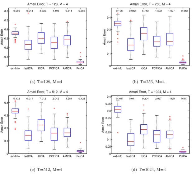
We generated the 5×5 orthogonal mixing matrix A randomly. The data matrix X was obtained as X=AS. The simulation was replicated 100 times. Our method, cICA-YW,
was compared with several popular existing ICA methods, including extended Infomax (Lee
et al., 1999), fastICA (Hyv¨arinen et al., 2001), Kernel ICA (KICA) (Bach and Jordan, 2003),
Prewhitening for Charateristic Function based ICA (PCFICA) (Chen and Bickel, 2005), and
(a)T= 128, M = 5 (b) T= 256, M = 5
(c)T = 512, M = 5 (d) T = 1024, M = 5
Following the practice of Bach and Jordan (2003) and Chen and Bickel (2005), we use the
Amari error between the true unmixing matrix and its estimate as a performance criterion
to compare the methods. Figure 2.1 shows the boxplot of the Amari error for each method
under the different sample sizes. The median computation time for each method is also
provided at the top of the corresponding boxplot. The cICA-YW procedure outperformed
the other ICA methods uniformly, and the advantage increased with sample size. As far as
the computing time is concerned, fastICA, Infomax, cICA-YW, and AMICA are the top four
fastest methods. In summary, cICA-YW provides very good estimates in a fairly short time.
The cICA-YW improved the performance over the other ICA methods by making use of the
temporal correlation structures within the sources.
2.3.2 Blind Separation of White Sources
We also examined the performance of wICA and cICA-YW when the sources are white noises.
In this second simulation study, three and five sources (M = 3,5) were generated under two
different sample sizes (T = 1024,2048). Three of the white noise sources were simulated from
uniform(−1,1), N(0,1) and double exponential(1) distributions. For the five-source setup, the two additional white noise sources were generated from t(3) and Weibull(1,1). Again
we randomly generated the orthonormal mixing matrix A. For reasons discussed in Section
2.2.4, the data were not prewhitened. We compared the performance of wICA, cICA-YW,
extended Infomax, KICA, PCFICA and AMICA over 100 simulation runs. Due to the ill
performance of the fastICA without prewhitening, the corresponding result is not included.
Figure 2.2 shows the boxplots of the Amari error for each method under the four simulation
setups, along with the median computation time in seconds. The AMICA performed best
followed by KICA for both sample sizes. The wICA and cICA-YW gave comparable results
in terms of the Amari distance when the number of sources is M = 3. For M = 5, wICA
and cICA-YW become comparable as the sample size increases. This confirms that the
model selection step of cICA-YW still works well for white noise cases. All the methods are
(a)T = 1024, M = 3 (b) T = 2048, M = 3
(c)T = 1024, M = 5 (d) T = 2048, M = 5
Figure 2.2: Simulation Study II: Performance Comparison for White Noise Sources. Sample sizes
2.3.3 Detection of Activated Brain Regions
Simulation Description
As discussed in Section 2.1, our research is primarily motivated by the application of fMRI
analysis. The current simulation study is designed to compare the performance of the various
ICA methods in analyzing a toy fMRI dataset. Below we describe the procedure for generating
the pseudo-fMRI data.
In this simulation, we first generated theV×M spatial map matrixAand theM×T time series matrix S, which were then multiplied to give the V ×T data matrix. In particular, we consider M = 4 temporal independent components that are of length T = 512; each
corresponding spatial map consists of 10 slices and each slice has 20×20 voxels, which results in a total of 4000 voxels for each spatial component. The final data matrix is 4000×512 in dimension.
The four temporal components are assumed to represent the task function, heart beating,
breathing, and noise artifact respectively. For the task function, we considered a simple
rest-activation block design with 18 seconds for each rest or rest-activation period (a frequency of
0.0052Hz); for the heart beat component, we used a harmonic function with a frequency of
1.71Hz; and for the breathing component, a harmonic function with a frequency of 0.3Hz.
These frequencies were chosen so that they have meaningful physiological interpretations.
The data were sampled every 0.3 seconds.
The four underlying independent temporal components were generated as follows:
• S1: Task function with noise = Task function +σ1Z1; • S2: Heart Beat with noise = sin(2π1.17t+ 1.61) +σ2Z2; • S3: Breathing with noise = sin(2π 0.3t+ 1.45) +σ3Z3;
• S4: S4(t) =−0.85S4(t−1)−0.7S4(t−2) + 0.2S4(t−3) +4(t), 4(t)∼i.i.d. uniform (−
√
3,√3).
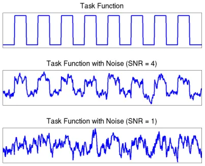
Figure 2.3: Simulation Study III: Task function at different SNR levels.
• Z1(t) = 0.8Z1(t−1) +1(t), 1(t)∼i.i.d. uniform (−√3,√3);
• Z2(t) =−0.6Z2(t−1)−0.5Z2(t−2) +2(t), 2(t)∼i.i.d. uniform(− √
3,√3);
• Z3(t) = 0.1Z3(t−1)−0.8Z3(t−2) +3(t), 3(t)∼i.i.d. uniform(−√3,√3).
It is worthwhile to consider different signal-to-noise ratios (SNR), since the sources of
interest can contain other irrelevant variabilities (Huettel et al., 2008). Figure 2.3 displays
the task function at different SNR levels. At a higher SNR level, we can easily distinguish the
task function, whereas it is harder to observe the task function at a lower SNR level. Hence,
in the current study, we considered four different setups: SNR=0.5, 1, 2, 4, and studied the
effects of SNR on the performance of the various ICA methods. In defining SNR, we follow
the suggestion of Bloomfield (2000).
Given a SNR level, for each of the first three source signals we calculated the corresponding
noise standard deviation asσj = q
Variance of the signal
Variance of the noise·SNR. The true temporal components at
SNR= 1 (blue solid line) are illustrated in Figure 5.5 below the noise-less task functions (red
dotted line). The spectral density curve for each component is also displayed at the top of
each panel, which is estimated using Welch’s power spectrum estimator (Welch, 1967). The
is displayed above the corresponding spatial map. We replicated the simulation 100 times for
each SNR.
Each voxel of a spatial map (i.e. a column of A) takes a binary value 1 or 0, where the
voxels with value 1 represent the regions that are activated by the corresponding temporal
stimulus, and the voxels of 0 indicate no activation. When plotting the spatial maps in
Figure 5.5, the activated voxels are colored white and the non-activated voxels are colored
black. For the spatial map corresponding to the noise temporal component, we randomly
selected 15% of the entries and coded them as 1. The voxels that correspond to none of the
temporal components will remain zero.
Analysis and Results
We first column centered each simulated data matrix (Hastie and Tibshirani, 2003). Due
to the high dimension of the data matrix, before applying the ICA methods, we then used
singular value decomposition (SVD) for dimension reduction (Petersen, K. and Hansen, L.K.
and Kolenda, T. and Rostrup, E., 2000). In particular, we extracted the leadingM=4 SVD
components which actually explained 99% of the raw data variance in all the simulation runs;
we then approximated the raw data matrix X using UeDeVe>, where the diagonal entries of
the diagonal matrixDe are the first M singular values, and the columns of Ue and Ve are the
first M left and right singular vectors, respectively.
Finally, the ICA algorithms were applied toXe =DeVe>to obtain the temporal component
matrixSband the mixing matrixA. In terms of decomposing the original matrixb X, the spatial
map matrix were estimated asAe =UeA, where each column is the spatial map correspondingb
to one recovered temporal component inS.b
The independent components extracted by ICA are ordered arbitrarily. To match each
recovered component with the original sources, we calculate the correlation between the
re-covered component and each of the 4 true temporal source signals, and the source that has
the largest absolute correlation is identified as the match.
To identify the activated voxels in each spatial map, we followed the suggestion of
(a) Task Function (b) Heart Beat
(c) Breathing (d) Noise
and dividing the standard deviation of the map. The voxels with|z|>1 then were identified as those that were activated.
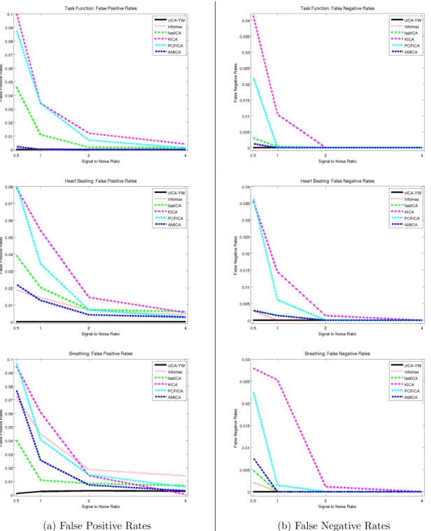
To gauge the performance of the ICA algorithms, we calculated the false positive and
false negative rates for each estimated spatial map. Each column of Figure 2.5 displays
the average of the false positive/negative rates over the 100 simulation runs under different
SNRs. The rows correspond to the spatial maps for the task function, heart beat, and
breathing, respectively. In each panel, six ICA methods are compared: cICA-YW (black
solid line), Infomax (red dotted line), fastICA (green dot line), KICA (margenta
dash-dot line), PCFICA (cyan dashed line), and AMICA (blue dashed line). The x-axis represents
the four different SNRs (0.5,1,2,4). The cICA-YW performed uniformly better than the
other methods, having the smallest false positive and false negative rates. In addition, the
false positive and false negative rates generally decreased as the SNR increased (except for
Infomax).
As a visual comparison of the detected spatial activation regions, we averaged the
esti-mated spatial maps across the first five simulations. The average spatial maps are plotted
for SNR=1 in the six rows of Figure 2.6 for the six ICA methods, respectively. In each row,
the average spatial maps for the first three independent components (task function, heart
beat, and breathing) are displayed sequentially. We observe that cICA-YW (Panels (a))
de-tected the spatial activation regions much better than its peers, whose noisier results for all
three source signals are clearly shown (when comparing with the true regions depicted in
Figure 5.5.)
We also conducted a similar simulation study for random event-related design. The task
function is random event-related contaminated with white noises (instead of correlated), where
the time intervals between two consecutive random events follow a Poisson distribution with
a mean of 4.5 seconds. (The other three sources follow the same models as in the above block
design; hence their noises are correlated.) The study results indicated that the cICA-YW
still leads the pack. These results along with the previous results for other values of SNR are
(a) False Positive Rates (b) False Negative Rates
Task Heart beat Breathing
(a) cICA-YW
(b) Infomax
(c) fastICA
(d) KICA
(e) PCFICA
(f) AMICA
2.4
Application to Real fMRI Data
2.4.1 Data Description
Experimental finger tapping data were obtained from our collaborators (reference omitted for
blinded review). The main neurological interest of the experiment was to identify the brain
regions responsible for the finger-tapping tasks. Two hundred MR scans were acquired on a
modified 3T Siemens MAGNETOM Vision system with a 3 second scan to scan repetition
time (TR). Each scan consisted of 49 contiguous slices containing 64×64 voxels. Therefore, we have 64×64×49 voxels at each of the 200 time points. Each voxel is a 3mm×3mm×3mm
cube.
The dataset was obtained by a control subject performing three different tasks
alterna-tively: rest, right-hand finger tapping, and left-hand finger tapping. Figure 2.7 (a) illustrates
the experimental paradigm. Each rest period lasted 30 seconds (10 time points) and each
fin-ger tapping task period lasted 120 seconds (40 time points). The block design task functions
are displayed as the black solid lines in Figure 2.7 (b). The red dashed lines stand for the
sine curves of the main task frequency (0.0033Hz).
2.4.2 Analysis
The dataset was first preprocessed using FSL (Smith et al., 2004). The preprocessing included
brain image extraction using the Brain Extraction Tool (BET), motion correction using
Mo-tion CorrecMo-tion with FSL’s Linear Image RegistraMo-tion Tool (MCFLIRT), slice time correcMo-tion,
spatial smoothing using FWHM 6mm×6mm×6mm, and highpass temporal filtering using a local linear fit. We removed the background voxels using the mask file obtained during
the preprocessing step. The dimension of the final data matrix was 68,963 voxels×200 time points.
FMRI images usually are of high dimension, especially in terms of the number of voxels.
To reduce dimension, we used thesupervised singular value decomposition(SSVD) algorithm
of Bai et al. (2008), which was shown to work better than SVD when doing ICA for fMRI.
(a) task paradigm
(b) Task Functions of right and left hand
Figure 2.7: (a) Experimental paradigm. (b) Task functions for right/left finger tapping (black solid lines) with task sine curve of main frequency (0.0033Hz, red dashed lines).
We then employed the entropy matching method (Li et al., 2006) implemented in the
Group ICA fMRI Toolbox (GIFT) (Calhoun et al., 2001) to select the number of independent
components to extract, which was suggested to be 13. Hence we extracted the leading 13
SSVD components, which formed a low-rank approximation of the fMRI data matrix as
e
U68963×13De13×13Ve>13×200, where the columns of Ue are the first 13 left supervised singular
vectors, the columns of Ve are the corresponding right supervised singular vectors, and the
diagonal matrixDe has the 13 supervised singular values on the diagonal. Finally, we applied
the six ICA methods (cICA-YW, Infomax, fastICA, KICA, PCFICA, and AMICA) to the
reduced data matrix, Xe = DeVe>, to estimate the temporal independent sources and the
mixing matrixA. The corresponding spatial maps were then estimated asb UeA.b
2.4.3 Results
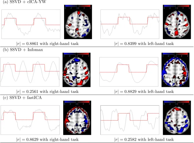
Figures 2.8 and 2.9 plot, for each of the six ICA methods, the first two temporal independent
can recover brain function-related signals of interest more accurately and sensitively than the
other ICA methods.
Each temporal component is displayed as a black solid line whereas the task function
with the highest absolute correlation is depicted by a red dotted line. To display the spatial
map, we transformed the subject’s anatomical brain structure into a reference image using
FMRIB’s Linear Image Registration Tool (FLIRT), which is built into FSL. Next, using
MRIcron (Rorden, 2007), several slices containing brain regions of interest were selected and
are shown with the component graphs. Activated voxels havingz <−1 were colored according to a blue-black color gradient and those having z >1 were colored according to a red-black
color gradient. A darker color represents less activation and a brighter color represents higher
activation. The areas withz <−3 orz >3 are colored blue and red, respectively.
Due to the sign ambiguity of ICA, we carefully interpreted the results taking into account
the signs of the spatial and temporal components. For the cICA-YW method, as shown in the
first column of Figure 2.8 (a), the left (contralateral) primary motor cortex (PMC), colored
red, was activated when the task was completed with the right hand (|r|= 0.8861 with the right-hand task). The meaning of negativezscores in fMRI data is subject to interpretation,
although one explanation may be that they represent decreased activation in a particular
region. Using this rationale, during the right hand task, the right PMC (blue) showed less
activation. The second column of Figure 2.8 (a) demonstrates that the method can detect
activity in bilateral PMC (red) during the left hand task (|r| = 0.8399 with the left-hand task).
The two components obtained by cICA-YW display activity in the corresponding
con-tralateral PMC, the lateral and medial parietal areas, and the anterior prefrontal. The PMC
is the final output center for motor tasks and thus activation in this region is consistent with
known biology and recent fMRI studies demonstrating increased activity in this region during
the performance of a variety of motor tasks (Haslinger et al., 2001; Gowen and Miall, 2007;
Lewis et al., 2007). In addition, recent imaging studies have shown the lateral and medial
parietal areas are involved in the postural configuration of the arm during the planning and
hands (see Vingerhoets et al. (2010)). Although referred to as one of the least understood
regions of the brain (Semendeferi et al., 2001), the anterior prefrontal region is implicated
in maintaining multiple tasks and their scheduling of operation (Koechlin and Hyafil, 2007).
The functions underlying both the parietal and frontal regions are integral parts of the
mo-tor task employed in the current study and thus activity in these regions is not unexpected.
The control subject is strongly right handed and it was interesting to note that in the PMC,
activity during the right hand task revealed only contralateral activity, whereas during the
left hand task the activity was more bilateral activity. These results suggest that use of the
non-dominant hand may require increased (bilateral) neural activity in the PMC.
Figure 2.8 (b) depicts the components with the strongest correlation with the right-hand
task (|r|= 0.2561) and left-hand task (|r|= 0.8829) obtained by Infomax. Both components have weaker correlations with the task functions than those obtained by the cICA-YW method
and also appear to include other signals (possibly physiological functions such as heart beat
and breathing). In addition, the spatial maps appear to include some artifacts which do not
have very clear biological meaning.
Figure 2.8 (c) shows the components obtained by fastICA. The left column displays the
component with the strongest correlation with the right-hand task (|r|= 0.8629). Activity is observed in the left contralateral PMC (red) but there also appears to be substantial
non-specific activity (in red) that may represent some artifact or correlation to functions
un-related to the task. Similar to cICA-YW, there was decreased activity in the right PMC (blue)
during this task, but there also was increased non-specific (blue) activity. The right panel
of Figure 2.8 (c) shows the best fastICA component to correlate with the left hand task.
The correlation obtained (|r| = 0.2582) is significantly smaller than that generated using our cICA-YM and it is unclear what the “decreased” (blue) activity represents biologically.
The spatial map also appears to include a potential artifact and does not match to the task
function of interest.
The components obtained by PCFICA are displayed in Figure 2.9 (a). The first
com-pared to our cICA-YW method, although this method does detect activity in appropriate
PMC structures.
Figure 2.9 (b) depicts the results obtained by KICA. The first IC (|r|= 0.4013 with right finger tapping) and the second IC (|r|= 0.6687 with left finger tapping) have much weaker correlations with the task functions compared to the cICA-YW method and also appear to
include other signals (possibly physiological functions such as heart beat and breathing). In
addition, the spatial maps appear to include some artifacts possibly caused by head motion.
The two components obtained by AMICA are reported in Figure 2.9 (c). The component
displayed in the left column of Figure 2.9 has weaker correlation with the right-hand task
(|r|= 0.3338). Although the correlation with left-hand task function (|r|= 0.9159) is higher than that obtained using our cICA-YM, and the activation is observed in the right
contralat-eral PMC (red), there also appears to be substantial non-specific activity (in red) that may
represent some artifact un-related to the task.
2.5
Conclusion
In this chapter we introduced a new ICA method, cICA-YW, and compared its performance
against several other established methods, including Infomax and fastICA. The method was
developed using the spectral domain approach to model the correlation structures of the
latent source signals, and the parameters were estimated via the Whittle likelihood procedure.
The advantage of taking into account the temporal correlation over the existing methods
was clearly demonstrated. The comparative simulation studies were conducted using a wide
variety of time series models for the source signals, including white noise, where our method
fared very well. In a real fMRI application involving motor tasks, the new ICA method also
detected relevant brain activities more accurately and sensitively.
We conclude this chapter by mentioning a possible future research direction. We intend
to extend our method to take into account both correlation structures within each source
and between the sources similar to those considered by subspace ICA and AMICA. Research
(a) SSVD + cICA-YW
|r|= 0.8861 with right-hand task |r|= 0.8399 with left-hand task (b) SSVD + Infomax
|r|= 0.2561 with right-hand task |r|= 0.8829 with left-hand task (c) SSVD + fastICA
|r|= 0.8629 with right-hand task |r|= 0.2582 with left-hand task
(d) SSVD + PCFICA
|r|= 0.7403 with right-hand task |r|= 0.7740 with left-hand task (e) SSVD + KICA
|r|= 0.4013 with right-hand task |r|= 0.6687 with left-hand task (f) SSVD + AMICA
|r|= 0.3338 with right-hand task |r|= 0.9159 with left-hand task
Chapter 3
Asymptotics of cICA-YW
3.1
Introduction
This section studies asymptotic properties of the cICA-YW method proposed in Chapter 2.
In many practical blind source separation problems, the sources have temporal correlation
structures. For example, in EEG studies, physiological signals such as heart beat or
respira-tory are usually periodic such information is not incorporated into the marginal-density-based
instantaneous ICA methods. In addition, the sources can be mixed with time delay, i.e. the
observation is a convolutive mixture of the source signals. The contextual ICA (Pearlmutter
and Parra, 1997) modeled the convolutive mixture as a multivariate version of the
autore-gressive process. In fact, this formulation is also referred to asconvolutive ICA. See Dyrholm
et al. (2007) and Chapter 8 of Comon and Jutten (2010) for a very thorough survey of this
topic.
In convolutive ICA, there are two categories: time domain approaches and spectral domain
approaches. The contextual ICA falls into time domain approaches, using logistic distribution.
D´egerine and Zaidi (2004) proposed to use Gaussian AR model on the time domain, and its
efficiency was shown by Doron et al. (2007). Lately, Dyrholm et al. (2007) proposed to
use multivariate ARMA models with order selection. Alternatively, Pham and Garat (1997)
proposed an ICA algorithm on the spectral domain and showed its sampling property with the
assumption that the spectra of the sources are known. In Chapter 2, this restriction has been
their method allows each source to have different AR orders, and thus makes convolutive ICA
procedure simpler.
Although there have been lots of research efforts that involve developing convolutive ICA
algorithms, the statistical sampling properties have not been deeply investigated so far. In
this chapter, we aim to establish the asymptotic properties of a convolutive ICA formulated
on spectral domain via the Whittle likelihood described in Chapter 3. The method is referred
to as cICA. In this chapter, our contribution is as follows: (a) proving the consistency and
the asymptotic normality of the cICA for linear processes with non-Gaussian sources via the
Whittle likelihood; (b) establishing the theoretical properties of cICA with spatial whitening
(or sphering); (c) investigate order selection of AR approximation via numerical study.
The rest of the chapter is structured as follows. Section 3.2 provides the background
to the multivariate spectral density estimation. Section 3.3 describes the proposed methods
for the correlated sources. Numerical studies for arbitrary full ranked mixing matrices are
reported in Section 3.4 with the order selection performances using different model selection
criteria. Proofs are given in Section 3.5. Some specific derivations and computations are given
in Section 5.1.
3.2
Preliminaries for Multivariate Time Series and Spectral
Density Estimation
3.2.1 Cumulants and Spectra
Consider an M vector-valued random variableX = (X1, . . . , XM)> with E|Xj|M <∞, j =
1, . . . , M, whereXj’s are real or complex. TheMth order joint cumulant,cum(X1, . . . , XM),
ofX1, . . . , XM is given by
cum(X1, . . . , XM) = M X p=1
(−1)p−1(p−1)!(EY j∈ν1
Xj)· · ·(E Y j∈νp
where the summation extends over all partitions (ν1, . . . , νp), p= 1, . . . , M. Ajoint cumulant
function of orderk of the series X(t) is given by
ca1...ak(t1, . . . , tk;X) =cum(Xa1(t1), . . . , Xak(tk)),
fora1, . . . , ak= 1, . . . , M and t1, . . . , tk= 0,±1, . . . .
If the span of dependence of X is small enough that
∞
X u1,...,uk−1=−∞
|ca1...ak(u1, . . . , uk−1;X)|<∞, (3.2.1)
we define thekth order cumulant spectrum,fa1...ak(r1, . . . ,rk−1;X), of series X by
fa1...ak(r1, . . . ,rk−1;X) = (2π)
−k+1
×
∞
X u1,...,uk−1=−∞
ca1...ak(u1, . . . , uk−1;X) exp{−i
k−1 X j=1
ujrj},
for rj ∈R, j = 1, . . . k−1, a1, . . . , ak = 1, . . . , M, k= 2,3, . . .. In particular, let the second
order cumulant spectrum matrix be defined by fXX(r) = [fjk(r;X)]j,k=1,...,M.
3.2.2 Discrete Fourier Transforms and the Periodograms
Suppose that we observeM vector-valued seriesX(t) = (X1(t), . . . , XM(t))>, t= 0, . . . , T−1.
Each component (row) of X, Xa, a = 1, . . . , M, is considered as a univariate time series.
Define the Fourier frequency by rk = 2πkT , k = 1, . . . , T −1. Then, the discrete Fourier
transform (DFT) for the univariate seriesXa, a= 1, . . . , M, is defined as
ϕ(rk, Xa, T) = T−1 X t=0
Xa(t) exp{−irkt}
=ϕa(rk,X, T), rk=
2πk
For M vector-valued seriesX, the DFT is defined by
ϕ(rk,X, T) = T−1 X t=0
X(t) exp{−irkt}
= (ϕ1(rk,X, T)· · ·ϕr(rk,X, T))>, rk=
2πk
T , k= 0, . . . , T −1.
The second-order periodogram of the univariate series Xa is given by
˜f(rk, Xa, T) =
1
2πTϕa(rk,X, T) ¯ϕa(rk,X, T),
where ¯c is the conjugate of a complex valued univariate variable c. For the r vector-valued
series X, the second order periodogram is given by
˜
f(rk,X, T) =
1
2πTϕ(rk,X, T)ϕ
∗(r
k,X, T)
= 1
2πT [ϕa(rk,X, T) ¯ϕb(rk,X, T)]a,b=1,...,M,
where a vectorϕ∗ is the conjugate transpose of the vectorϕ.
3.2.3 Parametric Spectral Density Estimation
This section describes a procedure for estimating the parameters of a stationary time series
via the Whittle likelihood, proposed by Whittle (1953).
Let X(t), t = 0,±1, . . ., be a univariate stationary time series with mean EX(t) = cX, EX2(t) < ∞, and continuous power spectrum fXX(r), −∞ < r < ∞. Without loss of
generality, letcX be zero.
In particular, we focus on the linear stationary process generated by
X(t) =
∞
X k=0
ak(t−k),
∞
X k=0
a2k<∞, a0 = 1,
spectral density, we have
fXX(r) = σ2
2π
∞
X k=0
akexp{−ikr} 2
, −π 6r6π.
Suppose that we observe X(0), . . . , X(T −1) and suppose that the spectral density fXX
depends on an unknown vector-valued parameter β. By the asymptotic independence and
the normality of the Discrete Fourier Transform (see, for example, Section 5.2 of Brillinger
(2001), or Section 10.3 of Brockwell and Davis (1991)), the Whittle log-likelihood function is
given by
LT(fXX) =−
1 2
T−1 X k=0
˜f(rk, X, T) fXX(rk)
+ lnfXX(rk) !
, rk=
2πk
T , (3.2.2)
where ˜f(·) is the periodogram defined previously.
Whittle likelihood based estimates have been investigated extensively in various schemes of
the parametrization including AR, MA and ARMA models and in the general settings
(Whit-tle, 1962; Walker, 1964; Ibragimov, 1967; Hannan, 1973; Rice, 1979; Hosoya and Taniguchi,
1982; Giraitis and Taqqu, 1999). For further details, see Dzhaparidze and Kotz (1986) and
Section 10.8 of Brockwell and Davis (1991). In our chapter, we investigate the theoretical
properties of a new ICA method based on maximization of the Whittle log-likelihood and the
parametrization of the spectral densities of the sources.
3.3
Main Results
This section describes the results for ICA based on temporally correlated (independent)
sources. Consider an M vector-valued stationary process X(t) = (X1(t), . . . , XM(t))>, t =
0,±1,±2, . . ., with mean zero,M ×M spectral density matrix fXX(r), r ∈ R. The spectral
density matrix fSS, DFT and periodogram of the source signals S(t) = (S1(t), . . . , SM(t))>, t= 0,±1,±2, . . ., are defined similarly. Note that since the sources are mutually independent, we have fSS = diag(f11, . . . , fM M), where fjj is the spectral density of thejth source.
independent stationary linear processes,Sj(t), such that
Sj(t) =
∞
X k=0
ajk(βj)j(t−k), j ∼WN(0, σj2),
for t= 0, . . . , T −1 and j = 1, . . . , M. For each j, the coefficients ajk is a function of a qj
dimensional parameterβj and aj0= 1 such that
∞
X k=0
a2jk(βj)<∞.
The power spectrum of Sj is given by
fjj(r;βj, σ2j) = σj2
2π ∞ X k=−∞
ajk(βj)e
−irk 2
, −∞<r<∞,
whereβ= (β>1,· · ·,βM>)>,σ2 = (σ21,· · · , σ2M)>. For simplicity, setθ= (vecW>,β>,σ2>)>. According to ICA equation,
S=WX, W=A−1, (3.3.1)
and the linearity of DFT, we can derive the Whittle likelihood in terms of the observed mixed
signals Xas
LT(W,θ;X) =−
1 2T
M X j=1
T−1 X k=0
eTjW˜f(rk,X, T)WTej
fjj(rk,βj, σ2j)
+ lnfjj(rk,βj, σj2) !
+ ln|detW|.
(3.3.2)
Then, we can obtain the estimates for the unmixing matrixW and the parameters in the
power spectraβ and σ2 by maximizing (3.3.2). Let Mbe an artibrary matrix with columns
M1, . . . ,Mm. Set
vecM=
M>1 . . .M>m
> ,
and define the Frobenius norm of M by kMk2
F = tr(MM