Stability of exomoons around the
Kepler
transiting circumbinary
planets
Adrian S. Hamers
1?, Maxwell X. Cai
2†
, Javier Roa
3‡
, and Nathan Leigh
4,5§
1Institute for Advanced Study, School of Natural Sciences, Einstein Drive, Princeton, NJ 08540, USA 2Leiden Observatory, Leiden University, PO Box 9513, NL-2300 RA Leiden, The Netherlands
3Jet Propulsion Laboratory, California Institute of Technology, 4800 Oak Grove Dr, Pasadena, CA 91109, USA
4Department of Astrophysics, American Museum of Natural History, Central Park West and 79th Street, New York, NY 10024, USA 5Department of Physics and Astronomy, Stony Brook University, Stony Brook, NY 11794-3800, USA
ABSTRACT
The Kepler mission has detected a number of transiting circumbinary planets (CBPs).
Al-though currently not detected, exomoons could be orbiting some of these CBPs, and they might be suitable for harboring life. A necessary condition for the existence of such exomoons is their long-term dynamical stability. Here, we investigate the stability of exomoons around
theKeplerCBPs using numericalN-body integrations. We determine regions of stability and
obtain stability maps in the (am,ipm) plane, wheream is the initial exolunar semimajor axis
with respect to the CBP, andipm is the initial inclination of the orbit of the exomoon around
the planet with respect to the orbit of the planet around the stellar binary. Ignoring any depen-dence onipm, for mostKeplerCBPs the stability regions are well described by the location of
the 1:1 mean motion resonance (MMR) of the binary orbit with the orbit of the moon around the CBP. This can be ascribed to a destabilizing effect of the binary compared to the case if the binary were replaced by a single body, and which is borne out by corresponding 3-body inte-grations. For high inclinations, the evolution is dominated by Lidov-Kozai oscillations, which can bring moons in dynamically stable orbits to close proximity within the CBP, triggering strong interactions such as tidal evolution, tidal disruption, or direct collisions. This suggests that there is a dearth of highly-inclined exomoons around theKeplerCBPs, whereas coplanar exomoons are dynamically allowed.
Key words: gravitation – planets and satellites: dynamical evolution and stability – planet-star interactions
1 INTRODUCTION
One of the exotic type of planetary systems detected by theKepler
mission are transiting circumbinary planets (CBPs), i.e., planets in nearly-coplanar orbits around a stellar binary (and nearly copla-nar with the plane of the sky), temporarily blocking the bicopla-nary’s light and giving a generally complex light curve (e.g.,Martin & Triaud 2015;Martin 2017). Currently, 10 confirmedKeplerCBPs are known in 9 binary systems (see Table1for an overview). These systems have revealed important clues for the formation and evolu-tion of planets and high-order multiple systems. For example, none of theKeplerCBPs are orbiting binaries with periods shorter than 7 d, which suggests the presence of a third star (Muñoz & Lai 2015;
Martin et al. 2015;Hamers et al. 2016), or could be indicative of coupled stellar-tidal evolution (Fleming et al. 2018).
A key question for the CBP systems is whether they would
? E-mail: [email protected]
† [email protected] ‡ [email protected] § [email protected]
be able to harbour life. As shown by various authors (Orosz et al. 2012a;Quarles et al. 2012;Kane & Hinkel 2013;Haghighipour & Kaltenegger 2013;Cuntz 2014,2015;Zuluaga et al. 2016;Wang & Cuntz 2017;Moorman et al. 2018), some of theKeplerCBPs are within the habitable zone (HZ). Some of theKeplerCBPs are giant planets and are unlikely to be able to sustain life; on the other hand, exomoons are prime candidates for celestial objects harbouring life (e.g.,Lammer et al. 2014;Sato et al. 2017;Dobos et al. 2017). Although techniques to observe exomoons have been developed, they have not yet been found (e.g.,Kipping 2009a,b;Kipping et al. 2012,2013a,b,2014; seeKipping 2014for a review). Given the abundance of moons in the Solar system, it is reasonable to assume that they exist.
A necessary condition for the existence of exomoons in the
KeplerCBPs is that they be long-term dynamically stable. In this paper, we address this issue by carrying outN-body integrations of exomoons orbiting around theKeplerCBPs (i.e., in S-type orbits around the CBPs,Dvorak 1984). We will show that stable configu-rations are possible for a wide range of parameters, and that the
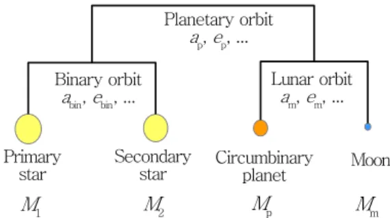
Figure 1.Schematic representation (not to scale) of the orbits of the stellar binary, the CBP, and its moon.
bility boundary is mediated by mean motion resonances (MMRs) with the stellar binary.
We note a previous work byQuarles et al.(2012), who consid-ered the dynamical stability (and habitability) of exomoons around Kepler 16. Our work can be considered as an extension ofQuarles et al.(2012), since we consider dynamical stability of exomoons for a wide range of inclination angles, and include all currently-confirmedKeplerCBP systems. Other theoretical efforts have re-vealed a number of interesting properties that distinguish CBPs from single-star host systems. For example,Smullen et al.(2016) showed using N-body simulations that the disruption of multi-planet systems tends to result in far more ejections relative to single-host systems, which more commonly lose their planets due to collisions upon becoming dynamically unstable. Typically, nu-merical simulations suggest of order 80% of outcomes correspond to ejections, and only 20% to physical collisions with the primary or secondary (Sutherland & Fabrycky 2016). In this chaotic regime, the distribution of escaper velocities has been well-studied and pa-rameterized in previous works, mostly in the context of scattering of single stars by super-massive black hole binaries (e.g.,Quinlan 1996;Sesana et al. 2006).
The structure of this paper is as follows. In Section2, we briefly describe the initial conditions and the numerical methodol-ogy used for theN-body integrations and for determining stability regions. The main results are given in Section3, in which we show the stability maps for theKeplersystems. We discuss our results in Section4, and we conclude in Section5.
2 METHODOLOGY
2.1 Initial conditions
Our systems consist of a stellar binary (massesM1andM2;
semi-major axisabin) orbited by a CBP (massMp; semimajor axisap).
In turn, the CBP is orbited by a moon (massMm; semimajor axis
am). A schematic representation (not to scale) in a mobile diagram
of the system (Evans 1968) is given in Fig.1.
We take the binary and planetary parameters for the currently-knownKeplersystems from various sources. The adopted orbital parameters are given for convenience and completeness in Table1. In most cases, the orbital angles are defined with respect to the plane of the sky. Note that the binary’s longitude of ascending node,
Ωbin, is defined to be zero. For several systems, the argument of pe-riapsis of the binary or the planet is not known. In this case, we set the corresponding values to zero. We do not vary the initial mean
anomalies of the binary and the planet (both are set to zero), but we do vary the moon’s initial mean anomaly (see below).
Kepler 47 harbors at least two CBPs, Kepler 47b and Kepler 47c (Orosz et al. 2012a), and there may be a third CBP, Kepler 47d (Hinse et al. 2015). Here, we do not consider Kepler 47d, which has not yet been confirmed. Also, we treat the two confirmed planets in Kepler 47 as separate cases, i.e., in each case we neglect the gravitational potential of the other CBP. We have checked that this assumption is justified by running simulations with both confirmed planets included, which yielded no significantly different results. Kepler 64, also known as Planet Hunters 1 (PH1), is a quadruple-star system; the binary+CBP system is orbited by a distant stellar binary (a visual binary) at a separation of ∼1000au(Schwamb
et al. 2013). In our integrations, we do not include the visual binary given the large separation between the two stellar binaries, and the relative scale of the inner CBP+planet triplet.
For each binary+planet system, we set up a fourth particle, the exomoon (henceforth simply ‘moon’), with massMm=qmMp,
whereqmis either 0.001 or 0.1, initially orbiting around the CBP
(for reference,qm'0.012 for the Earth-Moon system,qm'4.7×
10−5for Io-Jupiter, andq
m'0.12 for Pluto-Charon). We consider
40 values of the lunar semimajor axis,am, on an evenly-spaced grid,
with the lower and upper values depending on the system; typically,
amranges between 0.005 and 0.02au(see the figures in Section3.1
for the precise ranges ofamassumed for each system). The initial
eccentricity is set toem=0.01; we also carried out simulations with
higher initial eccentricities, but found no significant dependence of the stability regions onem.
The lunar argument of periapsis is set toωm=0; the longitude
of the ascending node is set toΩm = Ωp+π, such that the mutual inclination between the planet and the moon is
cos(ipm)=cos(ip) cos(im)+sin(ip) sin(im) cos(Ωp−Ωm)
=cos(ip+im), (1)
i.e., by construction, the mutual inclination between the planet and the moon isipm = ip+im. The inclination of the moon is set to
im =igrid−ip, whereigridis evenly spaced from 0 to 180◦with 40
values. We consider 10 different values of the lunar initial mean anomaly,Mm, evenly spaced between 0 and 2π. In summary, for eachKeplersystem in Table1, we carry out 40×40×10=16,000 integrations with differentam,ipmandMm. These sets are repeated
forqm=0.001 andqm=0.1 (binary case), and forqm=0.001 and
with the stellar binary effectively replaced by a point mass (single case, i.e., the primary stellar mass is replaced by M1+M2, and
the secondary stellar mass is reduced toM2 =1 kg, essentially a
test particle). This implies a total of 10×3×16,000=480,000 simulations for all 10KeplerCBP systems.
2.2 Determining stability regions
For our integrations, we use ABIE, which is a new Python-based
code with part of the code written in the C language for optimal per-formance (Cai et al., in prep.). ABIE includes a number of integra-tion schemes. Here, we use the Gauß-Radau scheme of 15th order (Everhart 1985), with a minimum time-step of 10−13, and a
toler-ance parameter of=10−8. The integrator incorporates a more
so-phisticated step-size control algorithm proposed byRein & Spiegel
in Section3.3. We check for collisions of the moon with the planet and stars, taking the collision radii to be the observed physical radii. In reality, the moon is likely tidally disrupted before colliding with the CBP or with the stars. The tidal disruption radius, however, de-pends on the density of the moon. Here, we choose a more general approach of setting the collision radii equal to the physical radii.
We carry out 4-body integrations of the binary+CBP+moon system for a duration oftend = 1000Pp, where Pp is the orbital
period of the planet around the binary. To investigate whether this integration time is sufficiently long, we show the stability regions below in Section3for different integration lengths. The (absolute values of the) relative energy errors in the simulations after 1000Pp
are typically on the order of 10−12, with maxima of∼10−10.
We determine stability maps using the following approach. For a given integration timetend and a point in the (am,ipm)
pa-rameter space, we define the orbit as ‘stable’ if the moon remains bound to the CBP (i.e.,am >0 and 0 ≤em<1) attendfor all 10
realizations with differentMm(green). If none of the 10
realiza-tions ofMmyield bound orbits to the CBP, then the orbit is flagged as ‘unstable’ (red). If the orbit remains bound for some, but not all realizations with differentMm, then we consider the orbit to be ‘marginally stable’ (yellow).
3 RESULTS
3.1 Stability regions
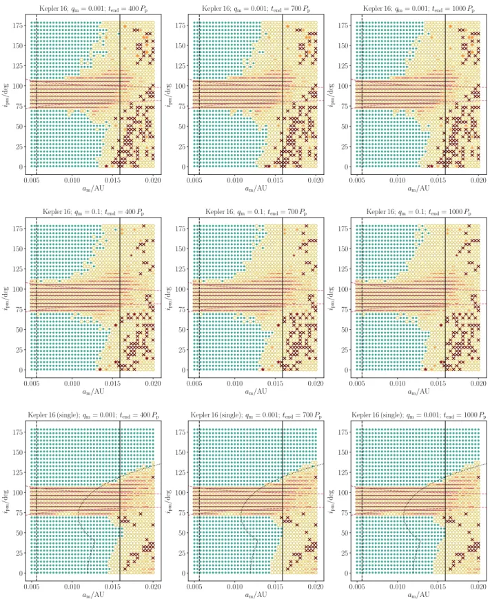
The main results of this paper are the stability maps shown in Figs2
and3, for Kepler 16, and the other 9KeplerCBPs, respectively. In these maps, each point in the (am,ipm) plane represents 10
simu-lations with different initialMm; green filled circles correspond to
stable systems, red crosses to unstable systems, and yellow open circles to marginally stable systems (see Section2.2for the defini-tion of stable, unstable and marginally stable systems). If a collision of the moon with the stars or the CBP occurred for one or more
Mm-realizations, then this is indicated with either the ‘−’ or ‘?’
symbols for collisions with the planet and the stars, respectively. We show the frequency for the most common collision type among the mean anomalies, and the color of these symbols encodes this frequency with respect to the 10 realizations ofMm(yellow to red
for 1 to 10). For collisions of the moon with the stars, the large and small ‘?’ symbols correspond to collisions with the primary and secondary star, respectively.
In Fig.2, the three panels in each row correspond to diff er-ent integration times: 400, 700 and 1000Pp. In the first and third
columns, the mass ratio of the moon to the planet isqm=Mm/Mp=
0.001, whereas in the second column,qm =0.1. The third column
corresponds to the single-star case, in which the stellar binary is replaced by a point mass. In Fig.3, the integration time is 1000Pp,
and the mass ratio isqm=0.001.
Generally, the maps can be characterized with a stable region at smallam, an unstable region at largeram, and a marginally
sta-ble region in between, as can be intuitively expected. There is also a dependence onipm, the mutual inclination between the orbit of
the moon around the planet, and the orbit of the planet around the inner binary — typically, high inclinations near 90◦
are less sta-ble than low inclinations (near 0◦and 180◦), and lead to collisions.
The larger instability near high inclinations can be ascribed to LK evolution, and this explored in more detail in Section3.3. Also, ret-rograde orbits (ipmnear 180◦) tend to be more stable than prograde
orbits (ipm near 0◦), in the sense that the marginal stability region
extends to a larger range inamfor retrograde orbits compared to
prograde orbits. This is consistent with the general notion that ret-rograde orbits are typically more stable than pret-rograde orbits owing to the higher relative velocities for retrograde orbits. However, we find that the ‘binarity’ of the stellar binary is also important, espe-cially for retrograde orbits. This is investigated in more detail in Section3.2.
As expected, the stability regions decrease for longer integra-tion times. However, there is little dependence on the integraintegra-tion time for the values shown, indicating that 1000Pp is sufficiently
long to determine stability in the majority of the parameter space. In the figures, we show for reference with the vertical blue dashed dotted lines the Hill radius (e.g.,Hamilton & Burns 1992; replacing the binary by a point mass), i.e.,
rH=ap(1−ep)
Mp
3(M1+M2)
!1/3
. (2)
Note thatrH does not lie within the range ofamshown in all
fig-ures; if the vertical blue dashed dotted line is not visible, thenrHis
larger than the largest value ofamshown. Although correct within
an order of magnitude, the Hill radius only captures the true sta-bility boundary within a factor of a few. This is not very surprising given that the Hill radius strictly only applies to the three-body case (with the binary replaced by a single body), and does not capture the inclination dependence.
3.2 Mean motion resonances
As mentioned above, the Hill radius does not accurately describe the boundary between stable and unstable orbits in the (am,ipm)
plane. Here, we consider an alternative simple analytic description of the stability boundary using an interpretation based on MMRs. First, we show in the third row of Fig.2and in Fig.4stability maps for integrations in which the stellar binary was effectively replaced by a point mass. For Kepler 16, the stable regions are significantly larger in the single-star case, especially for retrograde orbits. This shows that the binary tends to destabilize the moon, as is intuitively clear.
MMRs are due to commensurate orbital periods, and they have been studied in detail for single-planetary systems (e.g.,Peale 1976;Sessin & Ferraz-Mello 1984;Batygin & Morbidelli 2013;
Deck et al. 2013). For small bodies, MMRs are known to be desta-bilizing (e.g., the Kirkwood gaps in the Asteroid belt, e.g., Wis-dom 1983;Henrard & Caranicolas 1990;Murray & Holman 1997, and rings of Saturn, e.g.,Goldreich & Tremaine 1978;Borderies et al. 1982). The dynamics of MMRs in quadruple systems in the 2+2 configuration, which applies to our systems, are not well-understood (see Breiter & Vokrouhlický 2018 for a pioneering study which applies to the case of four bodies with comparable masses). In our configuration, we expect MMRs of the stellar bi-nary with the orbit of the moon around the planet to be important. Since the small-body limit applies, we also expect that these MMRs have a destabilizing effect. As shown by the ‘binary case’ stability maps, the binary indeed has a destabilizing effect, which is active foram <rH, until at a certain value ofamorbits are again stable.
Foram<rH, we expect the latter value to be mainly determined by
the 1:1 MMR with the stellar binary.
Using Kepler’s law, it is straightforward to show that the con-dition Pbin = αPm, where Pbin and Pm are the binary and lunar
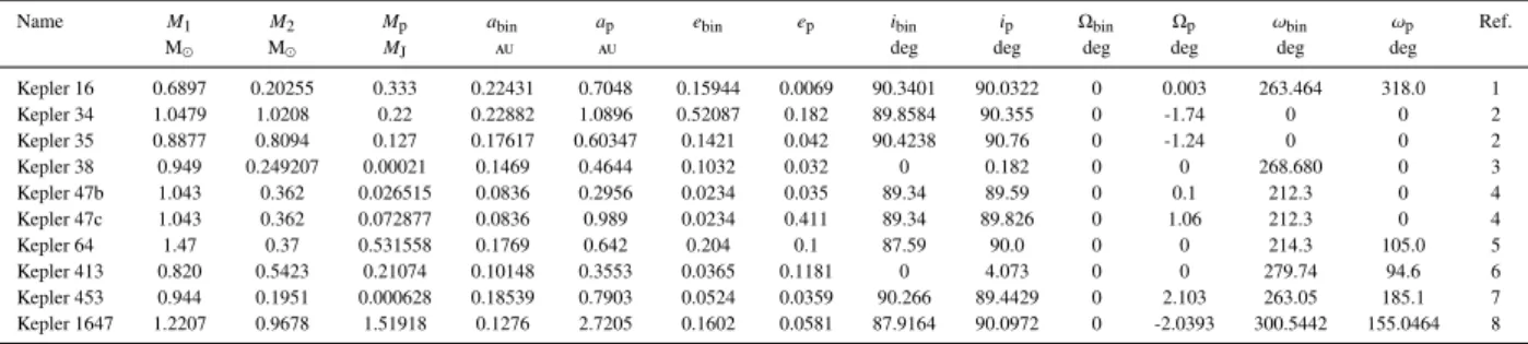
Name M1 M2 Mp abin ap ebin ep ibin ip Ωbin Ωp ωbin ωp Ref.
M M MJ au au deg deg deg deg deg deg
Kepler 16 0.6897 0.20255 0.333 0.22431 0.7048 0.15944 0.0069 90.3401 90.0322 0 0.003 263.464 318.0 1 Kepler 34 1.0479 1.0208 0.22 0.22882 1.0896 0.52087 0.182 89.8584 90.355 0 -1.74 0 0 2 Kepler 35 0.8877 0.8094 0.127 0.17617 0.60347 0.1421 0.042 90.4238 90.76 0 -1.24 0 0 2 Kepler 38 0.949 0.249207 0.00021 0.1469 0.4644 0.1032 0.032 0 0.182 0 0 268.680 0 3 Kepler 47b 1.043 0.362 0.026515 0.0836 0.2956 0.0234 0.035 89.34 89.59 0 0.1 212.3 0 4 Kepler 47c 1.043 0.362 0.072877 0.0836 0.989 0.0234 0.411 89.34 89.826 0 1.06 212.3 0 4 Kepler 64 1.47 0.37 0.531558 0.1769 0.642 0.204 0.1 87.59 90.0 0 0 214.3 105.0 5 Kepler 413 0.820 0.5423 0.21074 0.10148 0.3553 0.0365 0.1181 0 4.073 0 0 279.74 94.6 6 Kepler 453 0.944 0.1951 0.000628 0.18539 0.7903 0.0524 0.0359 90.266 89.4429 0 2.103 263.05 185.1 7 Kepler 1647 1.2207 0.9678 1.51918 0.1276 2.7205 0.1602 0.0581 87.9164 90.0972 0 -2.0393 300.5442 155.0464 8
Table 1.Initial conditions adopted for theKeplerCBP systems. See Fig.1for a schematic illustration of the definition of the orbital parameters. Here,i,Ωand ωdenote inclination, longitude of the ascending node, and argument of periapsis, respectively. The initial mean anomalies for the binary and planetary orbit were set toMbin=Mp=0. References: 1 —Doyle et al.(2011); 2 —Welsh et al.(2012); 3 —Orosz et al.(2012b); 4 —Orosz et al.(2012a); 5 —Schwamb
et al.(2013);Kostov et al.(2013); 6 —Kostov et al.(2014); 7 —Welsh et al.(2015); 8 —Kostov et al.(2016) .
can be written as
am,MMR=α
−2/3
abin
Mp
M1+M2
!1/3
. (3)
This expression has the same dependence on the masses as the Hill radius (equation2), but the dependence onap(1−ep) is replaced by
abin. For the 1:1 MMR,α=1; the corresponding values ofam,MMR
are shown in the stability maps with the solid black lines (the 2:1 and 1:2 resonances are shown with the black dashed lines).
As shown in the stability maps, the 1:1 MMR expression cap-tures the boundary between stable and unstable orbits well for most systems, especially for Kepler 35, 38, 47b, 64, and 413, which do not show a strong dependence onipmignoring the region of
LK-induced collisions near high inclinations. There are two notable exceptions: for Kepler 47c and Kepler 1647, the stability bound-ary is significantly larger thanam,MMR, and is more consistent with
rH. In the latter two systems, the CBP semimajor axis is relatively
large (more than several times the critical separation for dynamical stability, see, e.g., fig. 1 ofFleming et al. 2018), such that the ‘bina-rity’ (i.e., quadrupole moment) of the stellar binary is unimportant. In this case, the 1:1 MMR is expected to be weak, and it should not set the stability boundary. This is supported by a comparison of the maps for Kepler 47c and 1647 in Figs3and4, which reveals that the stability regions for these systems are virtually identical for the single and binary star cases.
3.3 Collisions and strong interactions
As shown in the stability maps, most collisions occur at high incli-nations around 90◦
. In Table2, we show the number of collisions of the moon with the planet (Ncol,p), the primary star (Ncol, ?1), and the
secondary star (Ncol, ?2, if applicable). Note that the total number of
integrations for eachKeplersystem is 16,000. The majority of the collisions are between the moon with the planet. Collisions of the moon with the stars are rare.
The high-inclination collision boundary has a ‘funnel’ shape which is symmetric around 90◦
, and becomes wider at smalleram.
This can be understood from standard Lidov-Kozai (LK) dynamics (Lidov 1962;Kozai 1962). In particular, in the quadrupole-order test-particle limit and treating the binary as a point mass, the maxi-mum eccentricity for zero initial eccentricity reached is given by
em,max=
r
1−5
3cos
2(i
pm). (4)
The implied periapsis distance is rperi,m = am(1−em,max) for
cos2(i
pm) < 3/5, and rperi,m = am(1 −em) (where the initial
value isem = 0.01) for cos2(ipm) ≥ 3/5 (the critical angles for
LK oscillations are set byipm = arccos(
√
3/5) ' 39.2315◦
and
ipm=π−arccos(
√
3/5)'140.7680◦
). Equatingrperi,mto the
plan-etary radiusRpgives a relation betweenamandipm, which is shown
in the stability maps with the red dashed lines. These lines gener-ally agree with the simulations at smallam, at which collisions are
driven by LK evolution. At largeram, collisions are due to
short-term dynamical instabilities rather than secular evolution, and be-come less dependent on inclination.
The stability maps shown above are based on Newtonian point-mass dynamics, neglecting strong interactions such as tidal effects and tidal disruption. Here, we briefly consider such interac-tions when the moon passes close to its parent planet (we do not consider strong interactions with the two stars, although, in princi-ple, unstable moons can also experience strong interactions with the binary, see, e.g.,Gong & Ji 2018for the case of scattering-induced tidal capture CBPs).
We evaluate the importance of strong interactions by compar-ing the periapsis distances of the moon to its parent planet to (mul-tiples of) the radius of the planet. In Fig.5, we show for Kepler 16 in the (am,ipm) plane the minimum periapsis distances,rperi,m,
recorded in the simulations. Here, we determinerperi,m=am(1−em)
from the minimum value among the systems in the (am,ipm) plane
that are stable (i.e., if the moon remains bound to the planet for all 10 realizations ofMm); if at least one of the realizations yielded an unbound orbit or a collision, then we setrperi,mto−0.001au, which
is indicated in Fig.5with the dark blue regions. Note that, due to a finite number of output snapshots, the true closest approach can be missed in some cases. For low inclinations, there is no excitation ofem, andrperi,m =am(1−em,0), whereem,0 is the initial
eccen-tricity. This is manifested in Fig.5as a linear relation for small in-clinations. For larger inclinations, LK evolution drives highemand
smallrperi,m, and collisions with the planet occur asipmapproaches
90◦.
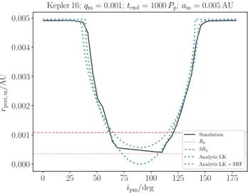
Also, we show in Fig.6a plot ofrperi,mversusipmfor a slice
inam, witham = 0.005au. The latter figure shows that the
de-pendence ofrperi,monipmforrperi,m>Rp is well described by the
canonical LK relation (equation4; green dashed line). The red dot-ted and dashed lines showrperi,m =Rp andrperi,m =3Rp,
respec-tively, whereRp =0.7538RJis the planetary radius (Doyle et al. 2011). Here, we take a factor of 3 to be indicative of the regime where tidal effects are important. Much closer in, tidal disruption is possible, or even direct collision. In the case shown for Kepler 16 and foram=0.005au, tidal effects are potentially important for
in-clinations near 60◦
and 120◦
. Direct collision occur for inclinations between∼75◦
and 105◦
0.0050 0.0075 0.0100 0.0125 0.0150 0.0175 0.0200
am/AU
0 25 50 75 100 125 150 175
ipm
/
d
eg
Kepler 34;qm= 0.001;tend= 1000Pp
Figure 3.Stability maps for nineKeplerCBP systems, similar to Fig.2. The name of the system is indicated above each panel. In all cases,qm =0.001, and the integration time is 1000Pp. The vertical black solid lines show the location of the 1:1 MMR of the moon with the binary (equation3); the vertical black dashed lines show the locations of the 2:1 and 1:2 MMRs. The red dashed lines show the boundary for collisions of the moon with the planet due to LK evolution, computed according to equation (4). The vertical blue dashed lines (not visible in all panels) show the Hill radius, equation (2).
3.4 Short-range forces
OurN-body integrations include the Newtonian point-mass terms only. Here, we investigate, a posteriori, the importance of short-range forces (SRFs) acting on the planet-moon orbit, in conjunc-tion with LK cycles. Such SRFs can include relativistic precession, and precession due to the quadrupole moment of the planet. In the case of Kepler 16, relativistic precession is completely unimpor-tant since the precession time-scale (on the order of Myr) is much
longer than the LK time-scale (on the order of tens of years; see also Table3).
However, the quadrupole moment of the planet can be impor-tant depending on the assumed structure of the planet, and, more importantly, its rotation rate. In Fig.6, we show with the blue dot-ted line the periapsis distancerperi,maccording to LK theory with
the addition of the quadrupole moment and tidal bulges of the planet (assumingqm=0.001). We computeem,maxby using energy
Figure 4.Similar to Fig.3, now for the single-star case (qm=0.001).
planet, we here assume a spin rotation period of 5 hr (a somewhat extreme case, given that for Kepler 16 the critical rotation period for centrifugal breakup is 2π/
q
GMp/R3p'3.4 hr), and an apsidal
mo-tion constant of 0.25. For these values, there is some deviamo-tion from the canonical relation equation (4), although, in this case,rperi,mis
not much affected unlessipmis close to 90◦.
To investigate the importance of SRF in allKeplerCBP sys-tems, we compute the associated time-scales in Table3. Approxi-mating the binary as a point mass, the LK time-scale can be esti-mated as (e.g.,Innanen et al. 1997;Kinoshita & Nakai 1999;
An-tognini 2015)
tLK=
P2 p
Pm
Mp+Mm+Mbin
Mbin
1−e2 p
3/2
, (5)
whereMbin≡M1+M2. The relativistic time-scale is (e.g.,Weinberg 1972)
t1PN=
1 6
amc2
GMp
Pm, (6)
Binary star (qm=0.001) Binary star (qm=0.1) Single star (qm=0.001)
Ncol,p Ncol, ?1 Ncol, ?2 Ncol,p Ncol, ?1 Ncol, ?2 Ncol,p Ncol, ?
Kepler 16 3235 106 129 3366 79 110 3193 0
Kepler 34 3120 3 3 3161 1 2 3395 0
Kepler 35 2589 26 22 2695 22 23 4376 0
Kepler 38 5743 0 0 5690 0 0 6059 0
Kepler 47b 4056 0 0 4246 0 0 4205 0
Kepler 47c 3115 0 0 3112 0 0 3281 0
Kepler 64 2442 55 73 2648 55 87 3319 1
Kepler 413 3155 15 10 3246 11 10 3958 0
Kepler 453 3047 0 0 3098 0 0 4727 0
Kepler 1647 1660 0 0 1702 0 0 1977 0
Table 2.Number of collisions of the moon with the planet (Ncol,p), the primary star (Ncol, ?1), and the secondary star (Ncol, ?2, if applicable), in the simulations withqm=0.001 (binary star case),qm=0.1 (binary star case), andqm=0.001 (single star case), and for an integration time of 1000Pp. The total number of integrations for eachKeplersystem is 16,000.
Figure 5.Minimum periapsis distances,rperi,m, recorded in the simulations in the (am,ipm) plane for Kepler 16. For unbound orbits or collisions, we setrperi,mto−0.001au, which is indicated with the dark blue regions in
the right-hand regions of each panel. The vertical black solid lines show the location of the 1:1 MMR of the moon with the binary (equation3), and the vertical black dashed line shows the locations of the 2:1 MMR. The red dashed lines show the boundary for collisions of the moon with the planet due to LK evolution, computed according to equation (4).
Fabrycky & Tremaine 2007)
t−TB1 =
15 8nm
Mm
Mp
kAM,p
Rp
am
!5
; (7)
t−1
rot=nm 1+
Mm
Mp
! kAM,p
Rp
am
!5 Ωp
nm
!2
, (8)
wherenm=2π/Pmis the lunar mean motion, andkAM,pis the
plan-etary apsidal motion constant. In equations (6), (7) and (8), we have set the eccentricity of the lunar orbit to zero. In Table3, we set
qm = 0.001 andkAM,p = 0.25, and we assume that the planet is
spinning at half its breakup rotation speed,Ωp,crit =
q GMp/R3p.
The time-scales are shown for two semimajor axes: am = a0,
Figure 6.Black solid lines: minimum periapsis distancesrperi,mfor Kepler 16 as in Fig.5, here for a slice in semimajor axis, i.e.,am=0.005au. Green
dotted curve: the analytic LK periapsis distance based on equation (4). Blue dotted curve: analytic LK periapsis distance based on a semianalytic calcu-lation taking into account the quadrupole moment and tidal bulges of the planet (assuming a spin rotation period of 5 hr and an apsidal motion con-stant of 0.25), and relativistic precession (which is not important). The red dotted and dashed lines showrperi,m=Rpandrperi,m=3Rp, respectively, whereRp=0.7538RJis the planetary radius (Doyle et al. 2011).
the smallest semimajor axis considered in the simulations, and
am=a1=am,MM, the location of the 1:1 MMR with the binary.
As shown in Table3, relativistic precession and tidal bulges are completely negligible for theKeplerCBP systems. Precession due to rotation, i.e., due to the quadrupole moment of the planet, are potentially important at small semimajor axes (in particular for Kepler 47b, 47c, and 453), although it should be taken into account that we assumed a somewhat extreme case of a near-critical rotation speed of the planet.
3.5 Summary plots
We summarize the results of the stability maps by determining the largest stable values ofam,am,crit, for each system and for a given
tLK/yr t1PN/Myr tTB/Myr trot/yr
a0 a1 a0 a1 a0 a1 a0 a1
K16 19.8 3.5 5.3 95.0 3.5 6400 5.4 557.5 K34 24.4 7.8 9.8 65.3 4.0 551.9 4.1 165.5 K35 4.0 2.3 22.4 57.8 6.7 78.9 4.0 14.9 K38 3.3 1.6 1061 3520 0.001 0.028 0.001 2.5 K47b 8.3 0.9 0.7 29.8 0.001 10.6 0.1 15.5 K47c 138 25.6 0.9 15.2 0.004 6.5 0.2 12.7 K64 9.0 2.6 2.6 21.0 13.2 2985 32.6 267.1 K413 14.5 1.2 0.2 12.5 0.003 192.0 0.427 59.2 K453 10.6 5.8 1147 3149 0.011 0.15 0.004 6.1 K1647 349 297 3.1 4.0 27.0 53.9 23.8 37.9
Table 3. Short-range precession time-scales for lunar orbits around the Ke-plerCBPs. The time-scales given are the LK, relativistic, TB, and rotation time-scales (see text for details), and are shown for two semimajor axes: am =a0, the smallest semimajor axis considered in the simulations, and
am=a1=am,MM, the location of the 1:1 MMR with the binary. Note that the units fortLKandtrotare yr, and Myr fort1PNandtTB.
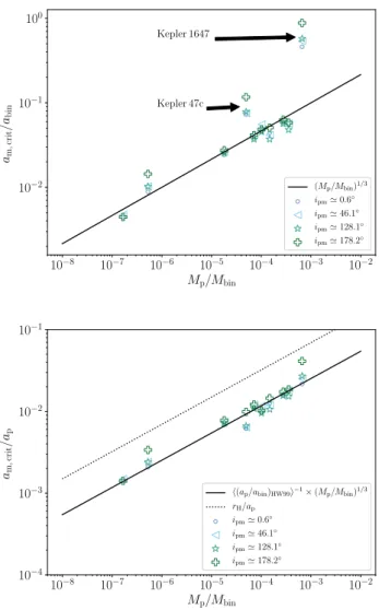
the planets and the stars (assumingqm =0.001). In particular, we
show in the top panel of Fig.7am,critnormalized toabin as a
func-tion ofMp/Mbin. Different symbols correspond to different
inclina-tions (refer to the legend). Note that high inclinainclina-tions, near 90◦
, are excluded since in this case there are no stable orbits in our simu-lations. Also plotted in the same panel with the solid black line is equation (3), the location of the 1:1 MMR. Most of the data points from the simulations match well with equation (3), again showing that the critical semimajor axis is close to the 1:1 MMR. Two no-table exceptions are Kepler 47c and Kepler 1647 (indicated in the figure with arrows), which, as mentioned in Section3.2, have rel-atively large planetary semimajor axes, such that the 1:1 MMR is weak and therefore does not set the stability boundary.
Alternatively, one can normalizeam,crit by ap. The resulting
points from the simulations are shown in the bottom panel of Fig.7. Again, most of the data are well fit by a power-law function of
Mp/Mbinwith a slope of 1/3, although the absolute normalization is
different. The black dashed line shows the Hill radius (equation2), which, as noted above, overestimates the criticalam for stability.
However, we can obtain a relation that better describes the data by using the fact that most of theKeplerCBPs are close to the limit for stability (i.e., stability of the planet in absence of the moon). In particular,
am
ap = am
abin
abin
ap = Mp
Mbin
!1/3 abin
ap
, (9)
where we used equation (3) with α = 1 (the 1:1 MMR). Subsequently, we replace abin/ap by h(ap/abin)HW99i−1, where
(ap/abin)HW99 is the critical CBP semimajor axis in units of abin
determined from the analytic fits of Holman & Wiegert (1999), and where the average is taken assuming a thermal eccentricity distribution of ebin and a flat mass ratio distribution (i.e., flat in
q=M2/M1). With these assumptions, we findh(ap/abin)HW99i−1'
0.252267, such that1
am
ap
'0.252267 Mp
Mbin
!1/3
. (10)
Equation (10) is shown in the bottom panel of Fig.7with the black solid line, and agrees with most of the data from the simulations.
1 Alternatively, one could computeh1/(a
p/abin)HW99i ' 0.25592, which gives nearly the same result.
10−8 10−7 10−6 10−5 10−4 10−3 10−2
Mp/Mbin
10−2
10−1
100 am , cr it /a b
in Kepler 47c
Kepler 1647
(Mp/Mbin)1/3
ipm≃0.6◦
ipm≃46.1◦
ipm≃128.1◦
ipm≃178.2◦
10−8 10−7 10−6 10−5 10−4 10−3 10−2
Mp/Mbin
10−4
10−3
10−2
10−1
am , cr it /a p
h(ap/abin)HW99i−1×(Mp/Mbin)1/3
rH/ap
ipm≃0.6◦
ipm≃46.1◦
ipm≃128.1◦
ipm≃178.2◦
Figure 7.Top panel: largest stable value ofam,am,crit, normalized toabin and plotted as a function ofMp/Mbin, whereMbin = M1+M2, for each system in the binary case withqm =0.001, and for a given value ofipm (refer to the legend). The solid black line shows equation (3), the location of the 1:1 MMR. Bottom panel:am,critnormalized toap. The black dotted line shows the Hill radius (equation2), and the black solid line shows the estimate equation (10) assuming the CBP is close to the critical boundary for stability.
4 DISCUSSION
4.1 Comparison to similar work
In the limit that the binary can be interpreted as a point mass, our results can be compared toGrishin et al.(2017), who considered the stability of inclined hierarchical three-body systems.Grishin et al.(2017) find the following expression for the limiting radii of stability as a function of the mutual inclination, i.e., in our case,
ipm,
rLKc (ipm,em,max)=ffudge31/3rHg(ipm)
−2/3
f(em,max), (11)
whereg(ipm) = cos(ipm)+
p
3+cos2(i
pm), and we take the
‘cor-rected’ function to be f(em,max) = 1/(1+e2m,max/2) withem,max
given by equation (4). The ‘fudge factor’ffudgeis set toffudge=0.5,
consistent withGrishin et al.(2017).
and the otherKeplerCBP systems, respectively. The absolute lo-cations of the stability boundaries in the simulations do not agree precisely with equation (11). However, the general shapes of the boundaries agree, with theam-boundaries increasing with
increas-ing ipm (i.e., retrograde orbits are more stable in the single-star
case), and a ‘bulge’ near high inclination. Note that equation (11) does not take into account collisions of the moon with the planet, which determine the stability boundaries in the simulations for in-clinations near 90◦
.
4.2 Implications of collisions
As shown above, most of the collisions in our simulations are col-lisions of the moon with the CBP, and occur at high inclination. However, some of the collisions are between the moon and the stars, and show no strong inclination dependence. Such collisions could enhance the metallicity of the stars, and/or trigger a speed-up of the stellar rotation in the case of a relative massive moon and a low-mass star. Speed-up of stellar rotation has been proposed to occur as a result of planets plunging onto their host star due to high-eccentricity migration (Qureshi et al. 2018).
5 CONCLUSIONS
We investigated the stability of moons around planets in stellar bi-nary systems. In particular, we considered exomoons around the transiting Kepler circumbinary planets (CBPs). Such exomoons may be suitable for harboring life, and are potentially detectable in future observations. We carried out numerical N-body simula-tions and determined regions of stability around theKeplerCBPs. Our main conclusions are listed below.
1. We obtained stability maps in the (am,ipm) plane, whereamis the
lunar semimajor axis with respect to the CBP, andipmis the
incli-nation of the orbit of the moon around the planet with respect to the orbit of the planet around the stellar binary. For most of theKepler
CBPs and ignoring the dependence onipm, the stability regions are
well described by the location of the 1:1 mean motion resonance (MMR) of the binary orbit with the orbit of the moon around the CBP (equation3). This can be ascribed to a destabilizing effect of the binary compared to the case if the binary were replaced by a single body, and which is borne out by corresponding 3-body inte-grations. For the two exceptions, Kepler 47b and Kepler 1647, the CBP semimajor axis is relatively large such that the 1:1 MMR is weak, and therefore it does not set the stability boundary.
2. For stable lunar orbits and high inclinations,ipm near 90◦, the
evolution is dominated by Lidov-Kozai oscillations (Lidov 1962;
Kozai 1962). These imply that moons in orbits that are dynami-cally stable could be brought to close proximity within the CBP, and experience strong interactions such as tidal evolution, tidal dis-ruption, or direct collisions. This suggests that there is a dearth of highly-inclined exomoons around theKeplerCBPs, whereas copla-nar exomoons are dynamically allowed.
3. Most of the collisions in our simulations are CBP-moon colli-sions, occurring at high inclination. Collisions with the stars are rare. However, if such collisions do occur, the stars in the binary might be enhanced in metallicity, and/or show an anomalously-high rotation speed.
ACKNOWLEDGEMENTS
This paper is part of theMoving Planets Aroundeducational book project, which is supported by Piet Hut, Jun Makino, and the RIKEN Center for Computational Science. ASH gratefully ac-knowledges support from the Institute for Advanced Study, The Peter Svennilson Membership, and NASA grant NNX14AM24G. This work was partially supported by the Netherlands Re-search Council NWO (grants #643.200.503, #639.073.803 and #614.061.608) by the Netherlands Research School for Astron-omy (NOVA). This research was partially supported by the In-teruniversity Attraction Poles Programme (initiated by the Belgian Science Policy Office, IAP P7/08 CHARM) and by the European Union’s Horizon 2020 research and innovation programme under grant agreement No 671564 (COMPAT project). MXC acknowl-edges the support by the Institute for Advanced Study during his visit. Part of this research was carried out at the Jet Propulsion Lab-oratory, California Institute of Technology, under a contract with the National Aeronautics and Space Administration.
References
Antognini J. M. O., 2015,MNRAS,452, 3610
Batygin K., Morbidelli A., 2013,A&A,556, A28
Borderies N., Goldreich P., Tremaine S., 1982,Nature,299, 209
Breiter S., Vokrouhlický D., 2018,MNRAS,475, 5215
Cuntz M., 2014,ApJ,780, 14
Cuntz M., 2015,ApJ,798, 101
Deck K. M., Payne M., Holman M. J., 2013,ApJ,774, 129
Dobos V., Heller R., Turner E. L., 2017,A&A,601, A91
Doyle L. R., et al., 2011,Science,333, 1602
Dvorak R., 1984,Celestial Mechanics,34, 369
Evans D. S., 1968, QJRAS,9, 388
Everhart E., 1985, in International Astronomical Union Colloquium. pp 185–202,doi:10.1017/S0252921100083913
Fabrycky D., Tremaine S., 2007,ApJ,669, 1298
Fleming D. P., Barnes R., Graham D. E., Luger R., Quinn T. R., 2018,ApJ,
858, 86
Goldreich P., Tremaine S. D., 1978,Icarus,34, 240
Gong Y.-X., Ji J., 2018, preprint, (arXiv:1805.05868)
Grishin E., Perets H. B., Zenati Y., Michaely E., 2017,MNRAS,466, 276
Haghighipour N., Kaltenegger L., 2013,ApJ,777, 166
Hamers A. S., Perets H. B., Portegies Zwart S. F., 2016,MNRAS,455, 3180
Hamilton D. P., Burns J. A., 1992,Icarus,96, 43
Henrard J., Caranicolas N. D., 1990, Celestial Mechanics and Dynamical Astronomy,47, 99
Hinse T. C., Haghighipour N., Kostov V. B., Go´zdziewski K., 2015,ApJ,
799, 88
Holman M. J., Wiegert P. A., 1999,AJ,117, 621
Innanen K. A., Zheng J. Q., Mikkola S., Valtonen M. J., 1997,AJ,113, 1915
Kane S. R., Hinkel N. R., 2013,ApJ,762, 7
Kinoshita H., Nakai H., 1999,Celestial Mechanics and Dynamical Astron-omy,75, 125
Kipping D. M., 2009a,MNRAS,392, 181
Kipping D. M., 2009b,MNRAS,396, 1797
Kipping D. M., 2014, preprint, (arXiv:1405.1455)
Kipping D. M., Bakos G. Á., Buchhave L., Nesvorný D., Schmitt A., 2012,
ApJ,750, 115
Kipping D. M., Hartman J., Buchhave L. A., Schmitt A. R., Bakos G. Á., Nesvorný D., 2013a,ApJ,770, 101
Kipping D. M., Forgan D., Hartman J., Nesvorný D., Bakos G. Á., Schmitt A., Buchhave L., 2013b,ApJ,777, 134
Kostov V. B., McCullough P. R., Hinse T. C., Tsvetanov Z. I., Hébrard G., Díaz R. F., Deleuil M., Valenti J. A., 2013,ApJ,770, 52
Kostov V. B., et al., 2014,ApJ,784, 14
Kostov V. B., et al., 2016,ApJ,827, 86
Kozai Y., 1962,AJ,67, 591
Lammer H., et al., 2014,Origins of Life and Evolution of the Biosphere,
44, 239
Lidov M. L., 1962,Planet. Space Sci.,9, 719
Martin D. V., 2017,MNRAS,465, 3235
Martin D. V., Triaud A. H. M. J., 2015,MNRAS,449, 781
Martin D. V., Mazeh T., Fabrycky D. C., 2015,MNRAS,453, 3554
Moorman S. Y., Quarles B. L., Wang Z., Cuntz M., 2018, preprint, (arXiv:1802.06856)
Muñoz D. J., Lai D., 2015,Proceedings of the National Academy of Sci-ence,112, 9264
Murray N., Holman M., 1997,AJ,114, 1246
Orosz J. A., et al., 2012a,Science,337, 1511
Orosz J. A., et al., 2012b,ApJ,758, 87
Peale S. J., 1976,ARA&A,14, 215
Quarles B., Musielak Z. E., Cuntz M., 2012,ApJ,750, 14
Quinlan G. D., 1996,New Astron.,1, 35
Qureshi A., Naoz S., Shkolnik E., 2018, preprint, (arXiv:1802.08260) Rein H., Spiegel D. S., 2015,MNRAS,446, 1424
Sato S., Wang Z., Cuntz M., 2017,Astronomische Nachrichten,338, 413
Schwamb M. E., et al., 2013,ApJ,768, 127
Sesana A., Haardt F., Madau P., 2006,ApJ,651, 392
Sessin W., Ferraz-Mello S., 1984,Celestial Mechanics,32, 307
Smullen R. A., Kratter K. M., Shannon A., 2016,MNRAS,461, 1288
Sutherland A. P., Fabrycky D. C., 2016,ApJ,818, 6
Wang Z., Cuntz M., 2017,AJ,154, 157
Weinberg S., 1972, Gravitation and Cosmology: Principles and Applica-tions of the General Theory of Relativity
Welsh W. F., et al., 2012,Nature,481, 475
Welsh W. F., et al., 2015,ApJ,809, 26
Wisdom J., 1983,Icarus,56, 51