A
CKNOWLEDGEMENTS
With the completion of this thesis being largely a collaborative process, I would first like to thank my advisor, Dr. Sèrgio Parreiras, for his persistent guidance and mentorship through-out the year. During our frequent meetings, he contributed invaluable insights into the development of the theoretical model and enabled me to understand the complex and latent economic phenomenon we were attempting to model. Without this continued instruction, it is unlikely this paper would have come to fruition in its current state.
Furthermore, I would like to express my gratitude toward Dr. Klara Peter, who spear-headed the yearlong honors seminar focused on methods in economic research and ensured progress was consistently being made toward the completion of the thesis. The assistance she provided in both structuring the empirical model (and introducing advanced econometric techniques) as well as interpreting the regression results greatly improved the quality of the statistical material presented in this paper.
A
BSTRACT
One of the most striking financial developments of the last five years involves the emergence and rapid adoption of digital currencies, with Bitcoin being the most prominent. This paper seeks to determine whether there is evidence of collusion between mining pools (coalitions of individuals that verify transactions for monetary returns). We first constructed a theoretical framework which modeled the mining activity as an infinitely repeated game between two competing pools. By devising payoffs in the form of value functions and applying the one shot deviation principle, we found that a collusive strategy was indeed an equilibrium–if certain conditions held. However, our empirical analysis offered more ambiguous results. Ultimately, our attempt to capture peer effects suggests the relationship between a mining pool and its competitors is negative and non-linear. While this could serve as evidence against collusive behavior, we also postulate alternate explanations that could account for the finding.
I. I
NTRODUCTION AND
M
OTIVATION
of Bitcoin transactions consistently exceeding $100 million and reputable retailers such as Microsoft accepting the digital currency, its influence on the global economy is poised to rapidly increase in the coming decades.
My research will focus on whether Bitcoin mining pools are engaging in collusive behavior in order to limit the amount of computational effort they must exert while maintaining prof-itability. Though the process of mining will be thoroughly explored in the following section, the activity revolves around firms (pools) verifying transactions and receiving newly minted currency as a reward. Over the course of the last five years, the most startling development in the mining community has been the formation of these mining pools and the rapid rate at which they rendered individual miners obsolete. These pools (coalitions of individuals and corporations that benefit from pooled computational power) have dramatically altered the process of mining and now serve as high-tech data centers that can compute mathematical functions billions of times per second.
Although such a topic may initially seem extremely esoteric and of little interest to economists, this naive attitude is incorrect. As was previously mentioned, digital currencies are becoming increasingly ubiquitous as consumers recognize the myriad of benefits asso-ciated with them (increased security, anonymity, etc), a fact reflected by the large volume of transactions completed daily. While Bitcoin has certainly received the largest share of media attention in recent years, innovative cryptocurrencies have continued to emerge (often modifying the mining process in intriguing ways) and offer consumers numerous ways to engage in this evolving market.
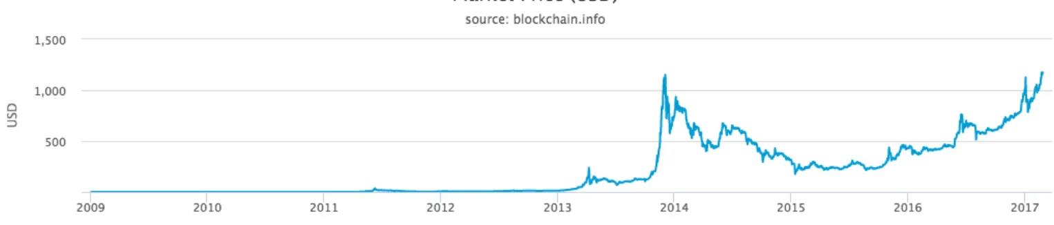
Fol-Figure 1:Graph depicting the rapid growth of Bitcoin’s valuation
Market value of a single Bitcoin since the currency’s launch in 2009. Measured in USD.
Figure 2:Graph depicting the number of Bitcoins in circulation
Number of Bitcoins in circulation since the currency’s launch in early 2009.
lowing a low and almost constant valuation for over four years, the price of a Bitcoin spiked in late 2013 as a result of increased interest in Chinese markets (ballooning past the $1000 mark), before adapting to more cautious market forces. Only in recent weeks has Bitcoin been able to eclipse these previous heights–attributable, to a large extent, to increased uncertainty in the United States and Europe.
this paper–while quite simplistic and plagued by limitations that will be expanded upon later–captures the peer effects and interdependence among pools by incorporating game theoretic tools. As future literature will no doubt need to account for these concerns, my model could serve as a basis for these works. On top of that, no other economist has made use of actual data made available from the blockchain, rendering the utilization here novel and contributory. However, the most significant contribution of this paper is in regards to the unintuitive and surprising empirical results generated through statistical testing. The negative relationship between the hash rate of a given pool and its competitors was an unexpected result and warrants further study in future work.
As the previous paragraph noted, the application of econometric methods yielded unan-ticipated results. One of the main findings is the aforementioned negative relationship between the hash rate of a particular pool and that of its peers. While it could be argued this serves as an argument against the existence of collusion between mining pools, the results also suggest its presence by indicating pools reduce their hash rates as a mining period elapses ("slacking off" in order to extend the duration of the round and prevent a large spike in the difficulty level). More discussion of the possible implications and explanations of this phenomenon will be provided in the results section. We also proposed a theoretical model which attempts to capture the interdependence between pools. According to the model, collusion is a subgame equilibrium if certain constraints on firm behavior and levels of computational resources hold.
whether data supports the hypothesis of collusion, describe the data source and the means of its acquisition, and provide discussion of the results obtained through regression analysis. Finally, we offer a conclusion that summarizes the main findings of the paper and suggests how future work could expand upon the foundation established here.
II. B
ITCOIN
M
INING
A
LGORITHM
While Bitcoin possesses many unique characteristics, none have attracted as much attention or become as recognizable as the process known as Bitcoin mining. As Bitcoin is a decen-tralized currency with no bureaucracy monitoring its use, the onus of verifying transactions falls to individuals collectively known as miners. As a comprehensive understanding of the nuances surrounding the process is unnecessary for the application of economic analysis, a description of the relevant aspects will now be provided.
When an individual submits a transaction utilizing Bitcoin–that is, they attempt to ex-change currency for a good or service–the result is not instantaneous. Since no trusted third party exists that can verify the consumer possesses the necessary funds and then facilitate the movement of bitcoins from one account to another, an alternate means of performing the task is necessary. This dilemma is resolved by perhaps the most significant innovation of Bitcoin: the delegation of this function to the mining community.
bitcoins. Following the successful addition of 2016 blocks to the blockchain, the target value is adjusted. Through this adjustment of the target value (commonly referred to as the mining difficulty), the creators of Bitcoin sought to limit the expansion of new currency and establish a means of distribution.
Figure 3:Graph depicting the evolution of the mining difficulty
Mining difficulty since Bitcoin launched in 2009. The creators of Bitcoin release an integer value to denote varying levels of difficulty, with higher numbers indicating adding a block to the blockchain is more difficult. Note that the massive increase in the mining difficulty is likely the result of two concurrent trends: the entry of new mining pools and technological advancements which allowed hash functions to be computed at lower costs.
Along with the reward of new currency, miners also have the potential to receive a small transaction fee for each verification they perform. When engaging in a transaction, con-sumers have the option of including a small fee that will be provided to miners upon success-ful addition of a block containing that transaction to the Blockchain. As there is no sales tax associated with Bitcoin, this minuscule fee ($.41 for an average sized transaction) is decided by the individual making a purchase, who may decide to provide no reward to miners. There is, however, a strong negative correlation between the size of the transaction fee and the amount of time for the transaction to be processed.
thereby allowing currency to be generated an unnatural rate. Although such subversion might have been possible in the initial days of the cryptocurrency, such manipulation is now entirely unnecessary. With the daily transaction value exceeding $100 million and exhibiting an upward trend, a supply of available transactions is constantly available, thereby allowing pools to perform hash functions as often as they desire.
Finally, I will address one of the primary concerns that has arisen in the Bitcoin community in recent years. With the advent of massive mining pools possessing incredible computational power, there exists a plausible scenario in which a pool amasses enough concentration (measured as their proportion of the hash rate) to insidiously manipulate the cryptocurrency. As Halaburda and Sarvary note in their pioneering examination of the ascent of Bitcoin:
The main role of the proof-of-work is to ensure immutability of the ledger. The solution to the puzzle becomes a part of the block being added to the blockchain. Importantly, the solution depends on the blocks preceding it in the blockchain. Suppose you wanted to go back and change a transaction, for example replacing the recipient of the bitcoins being sent with yourself. This would change one of the past blocks, meaning you would need to redo the proof-of-work for that block to make it a valid addition to the blockchain. Even more important, you would also need to redo the proof-of-work for all the blocks that follow it. You would need 51 percent of the computing power of the whole network to outper- form other miners in order to successfully put fraudulent blocks into the blockchain. Gaining such computational power is very costly, which was the intent in Bitcoin network design [4].
Although the current distribution of mining pool hash rates may alleviate such fears and indicate concern is unwarranted, a more thorough analysis suggests otherwise. As recently as 2014, the mining pool ghash.io possessed the capability to operate at this concentration and potentially compromise the entire currency. Recognizing the immense danger this posed, individuals within ghash.io self-regulated and joined alternate pools. In the two years since, numerous competitors have emerged and the highest concentration of any pool currently stands around 20%.
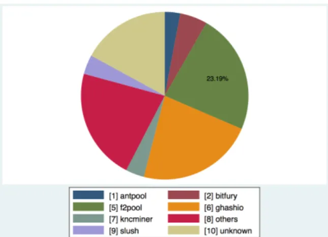
Figure 4:Pool Concentration in September 2014
Distribution (measured by proportion of overall hash rate) of mining pool concentration in September 2014. Note that certain pools had not come into existence yet, and thus possess no share of overall hashing.
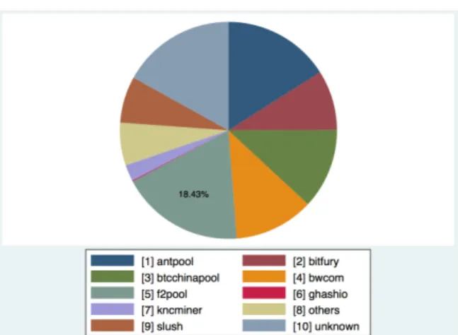
Figures 4 and 5 portray the concentration of mining pools (measured by their proportion of the overall hash rate) at periods approximately two years apart. As evidenced by the pie charts, this period witnessed the emergence of new pools and a trend toward decentralization among any major pool.
III. R
ELATED
L
ITERATURE
Figure 5:Pool Concentration in September 2016
Mining distribution in September 2016. The emergence of additional pools appears to have diminished the dominance of any particular pool.
Bitcoin is determined [1]. While such a topic is not directly related to my own, the paper provided guidance in how to specify my theoretical model and enhanced my understanding of the various processes underlying the cryptocurrency. The authors begin by presenting a simplified market (devoid of investors) in which the value of Bitcoin in determined by the laws of supply and demand. In this scenario, a steady state exchange rate emerges in which the ratio of expected transaction volume is equal to the supply of Bitcoins. With this established, they then allow for the introduction of investors and find that these individuals would exit the market once the steady state equilibrium is reached.
Since there is a minimal amount of economics research on the topic of Bitcoin, the remaining relevant papers I have considered simply incorporate game theoretical and time series elements that have been applied to varying industries and situations. These papers, while covering topics completely unrelated to Bitcoin, have offered insight into structuring my theoretical and empirical models.
game in which each is able to exert high or low effort during each round. Ultimately, the collusive equilibrium (exerting low effort) is supported only if the lead of a given firm remains moderate. If a firm possesses a large lead, they have an incentive to choose high effort in an attempt cement their dominance and further crush their opponent. On the other hand, when a lead is small both players have an incentive to deviate from a collusive stratagem: the player with the lead seeks to hold off their opponent, while the lagging opponent observes an opportunity to converge with the leader. Since the specification of my model was closely aligned with Hörner, we will determine if our model supports similar conclusions.
Although not a major focus of my research, another paper sheds insight onto the decision for individuals to transition from single miners into coalitions of miners. Armando Gomes proposes a model which may provide illumination on the topic [3]. In the paper, he describes the process of coalition formation as a repeated game in which players have the option to enter into new contracts at the end of each round. His analysis concludes by demonstrating that the strategy profile of each player results in a Markov perfect equilibrium in which the actions of the players in round t depends only on the state at the end of the previous round (t-1). Moreover, Fonseca and Normann jointly explore the effects of explicit and implicit collusion in markets exhibiting characteristics of oligopolies [2]. Not surprisingly, the theoretical model they construct implies that explicit collusion often leads to higher prices and less defection from collusive behaviors.
paper, dealing predominately with abstract game theory and complex mathematics, proposes an iterative algorithm for computing a Markov Perfect Equilibrium from a value function that recursively determines the payoff in repeated game of arbitrary length. Additionally, a lauded paper published by Weintraub, Benkard, and Van Roy applies similar techniques to industries characterized by the presence of numerous firms [9]. Rather than computing the Markov equilibrium–which proves extremely difficult for many applications–the researchers introduce what they refer to as an oblivious equilibrium. Utilizing this concept, they propose a method in which the actions of a given firm depend only on the current state of the firm and the long-run averages of the industry; that is, firms dismiss knowledge of the current state of their competitors. This simplification enables equilibria to be computed with significantly greater ease, while still accounting for the existence of states that influence of behavior of participants.
Additionally, I have consulted sources incorporating time series analysis in order to improve my knowledge of the discipline and gain insight into how to structure my empirical model. Mall utilizes techniques that resemble those I will need to employ to effectively estimate the degree of collusion between Bitcoin mining pools [6]. In investigating the effect of foreign investment on Pakistan’s growth over a period spanning over three decades, Mall must include the effects of lag in his model to compensate for the endogeneity present between his dependent and independent variables. Although his research topic bears little to resemblance to my own, I too must incorporate lags as a result of the high degree of covariance between my regressors, and can thus use his empirical model as reference when constructing mine.
outlining the differences between endogenous, exogenous, and correlated effects, Manski delivers a staggering assertion: that inference of group influence is not possible unless the researcher possesses prior information that specifies the composition of reference groups. By noting that the "prospects are poor to nil" if such characteristics remain elusive, he concludes that only more advanced theory or the collection of richer data can alleviate these concerns. As my analysis will attempt to capture and estimate a peer effect (how the behavior of a particular mining pool influences their peers), I will need to note the limitations and concerns described by Manski when specifying my empirical model and interpreting regression results.
Overall, the availability of similar research has provided tremendous aid in completing this paper. Although few economists have thoroughly analyzed Bitcoin or any of its attributes, the existing body of work on competitive environments served as a basis for our work. How-ever, certain limitations and caveats remain. Most notably, accurately measuring the peer effect remains a difficult endeavor and is fraught with error. Additionally, the uniqueness of Bitcoin mining (in which the actions of pools in one round will influence the difficulty and computational costs in subsequent rounds) differs from a standard perfectly competitive marketplace, thus rendering some aspects of current literature inapplicable.
IV. T
HEORETICAL
M
ODEL
assume the investment decision made by the firm is a binary decision in which
eit 2{1,e} (1)
That is, the pool must decide between making no investment in capital (in which eti =1) or increasing their stock by a factor of e, which is greater than 1. Thus, assuming no depreciation of capital occurs, the capital possessed by a pool can be defined as
kti=kit°1·eit (2)
During each period of the repeated game, the two pools compete to successfully include a block within the Blockchain, thereby accruing the reward of new Bitcoins. As a result of the simplifications imposed in the model, the payoff of a pool in a particular round is dependent only on three factor: the capital of that particular pool in round t, the capital of its competitor, and the current difficulty. These three aspects represent a state in an automata (often referred to as a finite state machine) and completely determine the outcome received both pools. Through this mechanism, the simple combination of the three is sufficient to generate the current state and payoff. Thus, the state in period t is represented by the following ordered triple:
st =(kt1,k2t,dt) (3)
Given a particular state, st, the utility derived by either pool can be easily computed. Assuming a pool experiences a utility of 1 if they succeed in the mining endeavor and a utility of 0 in the case of failure, the utility function ui(st) can be defined by its expectation:
ui(st,et)= k i t·eit
k1
t ·e1t +k2t ·e2t +dt
(4)
block to the Blockchain.
Suppose that the rate of failure– that is, the probability that neither pool computes an acceptable hash function– is defined by∞and the adjustment of the difficulty mechanism forces a constant rate. This rate of failure can be specified as follows
∞= dt+1
k1
t +k2t +dt+1
(5)
Solving for dt+1, we find the law of motion for the difficulty to be
dt+1=
∞(k1t +kt2)
1°∞ (6)
We can similarly define the rate of success,Ω(the probability that either pool succeeds in adding a block to the Blockchain in round t)
Ω= k
1
t +k2t
k1
t +kt2+dt
(7)
Two straightforward strategy profiles immediately present themselves when considering this model. In the first—the collusive strategy—the two pools continually abstain from investing in additional capital, remaining satiated with the status quo. Assume that the initial level of difficulty,d0satisfies a steady state equilibrium–that is, it is defined by equation 6. In
this case, the value function representing the payoff of pooli is:
Vi(st)=ui(st)+±Vi(st+1)=
1
X
n=0
±nui(st+n)= (8)
=X1
n=0
±n k
i
0
k01+k02+dn = 1
X
n=0
±n k
i
0
k1 0+k20+
∞
1°∞(k10+k20)
=
= k
i
0
(k10+k20)(1+1°∞∞)· 1
1°± (9)
k1
k2
k1·e
k2
k1·e2
k2·e
k1·en
k2·en°1
(e,1) (1,1)
Figure 6:The collusive strategy profile
Pools following the collusive strategy profile will refrain from investing in each round, thereby main-taining their initial stocks of capital and rendering the mining difficulty constant. Once one pool deviates from the strategy and invests, both pools transition to the competitive strategy profile and invest in each subsequent round
of capital and the difficulty) remaining constant in each period. If either firm were to deviate from this strategy by investing in additional capital, the opponent would merely respond by choosing to invest in each subsequent round. Figure 6 depicts this strategy profile.
On the other hand, there could exist a strategy profile—the non-collusive strategy—in which both firms choose to invest in every round, thereby increasing their stock of capital by a factor ofein the transition from period t to t+1. In this scenario, the difficulty path satisfies:
dt+1= ∞
1°∞((k
1
0+k20)·et+1) (10)
The value function would be specified as:
Vi(st)=ui(st)+±Vi((k1t ·e,k2t ·e,
∞(k1t +k2t) 1°∞ ))=
1
X
n=0
±nui(st+n)= (11)
=X1
n=0
±n k
i
0·en+1
(k01+k20)·en+1+d
n = 1
X
n=0
±n k
i
0·en+1
(k1
0+k02)·en+1+
∞
1°∞(k01+k02)·en
k1
k2
k1·e
k2·e
k1·e2
k2·e2
k1·en
k2·en
(e,e) (e,e)
Figure 7:The non-collusive strategy profile
In the competitive (non-collusive) strategy profile, pools invest in each round.
= X1
n=0
±n e
n·(ki
0·e)
en((k1
0+k02)·e+
∞
1°∞(k
1 0+k02))
= k
i
0·e
(k01+k20)·(e+1°∞∞)· 1
1°± (12)
With both pools perpetually investing in further capital, observe that the difficulty must consequently adjust in order to retain the constant rate of failure. Therefore, the benefit resulting from investment is reduced, as an increased hash rate is required to compensate for the greater computational challenge. Figure 7 depicts this strategy profile.
V. E
QUILIBRIUM
A
NALYSIS
LetVC(k,d) denote the value function when the stock of capital isk=(k1,k2) and the
diffi-culty is set at d, players are using the collusive strategy profile, and no player has deviated. Also, letVN(k,d) denote the value function when the stock of capital isk=(k1,k2), players
are using the non-collusive strategy profile, and no player has deviated. Assume these value functions adhere to the law of motion of the difficulty previously defined: when the players collude no change occurs and when they invest the difficulty adjusts accordingly. Note that when a player first deviates when the collusive profile is being played, say player 1 deviates, the value of the continuation game isVN(k1·e,k2,1°∞∞(k1·e+k2)).
For the collusive strategy profile to be a subgame perfect Nash equilibrium, by the one shot deviation principle, it has to be the case that:
period).
2. If some player invested before, then no player has an an incentive to not invest.
Formally, these incentive constraints are (we focus on player 1, the conditions for player 2 are analogous).
V1C(k1,k2,d)∏u1(k1·e,k2,d)+±·V1N(k1·e,k2, ∞
1°∞(k
1
·e+k2)) (C1)
V1N(k1,k2,d)∏u1(k1,k2·e,d)+±·V1N(k1,k2·e, ∞
1°∞(k
1+k2·e)) (C2)
Unfortunately, as a result of neglecting to include a cost function dependent on a pool’s given level of capital, condition 2 is always fulfilled, meaning only the competitive strategy is an equilibrium. In order to remedy this problem, we can modify the original utility function as follows:
ui(st,et)=
kit·eit
k1t ·e1t +k2t ·e2t +dt °
c·kit·eit (13)
This formulation captures the fact that investing in additional capital leads to higher costs (in the form of electricity needed to power greater computational resources) in all subsequent rounds and may serve as a deterrent from repeated investment.
Furthermore, we introduce a more sophisticated strategy profile that that involves the notion of a punishment phase. Under this strategy, which can be thought of as a variation of tit-for-tat, both players will initially behave collusively and avoid investing in additional levels of capital. Once one of the participants deviates from the strategy by investing, the other will initiate a punishment by investing in the subsequent round, effectively eliminating the advantage gained by the opposing pool.
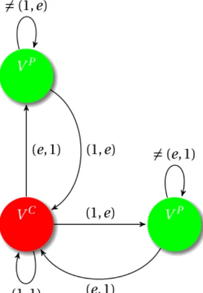
VC VP VP
(1,e)
(1,1)
6=(e,1)
(e,1) (e,1)
6=(1,e)
(1,e)
Figure 8:Automata representing the punishment strategy
Pools adhering to this strategy will initiate a punishment if their opponent deviates from collusion and invests in additional capital. As evidenced by the automata, if either player invests while in the collusive state (the red node), the players will transition to a state in which a punishment is enacted. If the deviator accepts the punishment without investing again, collusion will be resumed in the following round.
resuming the collusive strategy with the higher cost. Second, a pool that invests in a given round should find not deviating during the punishment phase must yield at least as much utility as deviating once again and incurring yet another punishment. And third, the player initiating the punishment must find the utility of following through with the punishment (thereby incurring a higher cost in the process) at least as advantageous as allowing this transgression to occur without consequence. These three conditions can be expressed through corresponding value functions.
Again, letVC(k,d) denote the value function when the stock of capital isk=(k1,k2) and d
an analogous function could be provided for the second pool:
V1P(k,d)= k
1
k1+k2·e+d·(k1+k2)°c·k1+±V1C(k1,k2·e,
∞ 1°∞(k
1+k2·e)) (14)
If the collusive strategy is indeed a subgame perfect equilibrium, by the one shot deviation principle, the following inequality must hold:
V1C(k1,k2,d)∏ k
1·e
e·k1+k2+d°c·k1·e+±V1P(k1·e,k2,
∞ 1°∞(k
1·e+k2)) (15)
This equation corresponds to the first condition outlined above and must clearly hold if constant collusion is an equilibrium.
In addition to the aforementioned condition, it must also be the case that a player being punished chooses to resume the collusive strategy profile rather than deviating for a second time. Assume that pool 2 deviated in the prior round and is in the process of being punished by pool 1. Again, the one shot deviation principle can be applied to yield the following inequality:
V2P(k1,k2·e,d)∏ k
2·e2
e·(k1+k2·e)+d°c·k
2·e2+±VP
2 (k1·e,k2·e2,
∞ 1°∞(k
1·e+k2·e2)) (16)
Finally, the player executing the punishment must have enough of an incentive to follow through with the investment, in spite of the higher cost they will then incur in each sub-sequent round. The value function presented represents the scenario in which player two deviated from the collusive strategy in the previous round and player one is responding.
k1·e
(k1+k2)·e+d°c·e·k1+±V1C(k1·e,k2·e,
∞ 1°∞·e(k
1+k2))∏VC
1 (k1,k2·e,d) (17)
com-plexity of the equations and large number of variables, we assumed e was equal to 1.5 and ∞was .1. With these assumptions and other constraints imposed, the system yielded more favorable results than our previous endeavor. The collusive strategy (forgoing investment in all periods) became an equilibrium if certain numerical constraints held for the stock of capital of the pools, the discount factor (±), and the cost constant c. While the values necessary for this equilibrium will not be presented as a result of the the high level of intricacy and breadth, the economic intuition and reasoning will.
A primary finding is that the pools must be relatively close in capital stock for collusion to hold as an equilibrium. Such a constraint is likely due to the multiplicative nature of the capital investment. Since a pool is able to scale their current inventory (rather than merely add a constant amount), the increase in capital is determined by the current level possessed. Therefore, if a pool has a large enough lead, the increased probability of successfully adding a block to the blockchain may outweigh the higher cost burden associated with this increased level of capital. Such a finding both affirms and disagrees with Horner’s analysis of firms in competitive situations, in which he assets that effort is exerted either when a lead is large (to further dominate the opponent and force them out of the market) or a lead is small (to regain dominance) [5]. Although we found that collusion breaks down if a large lead exits, failure to invest happens when a lead is relatively small.
Additionally, the conditions are ripe for equilibrium when the discount factor is close to 1. Intuitively, this result (which suggests that pools value future profits nearly as much as current profits) coincides with economic theory, as pools with such preferences would be unwilling to sacrifice long-term rewards for short term gains.
pool must be willing to follow through with the punishment, and a large increase in their costs would discourage such action. It should be noted that this conclusion is somewhat unrealistic, as a high enough cost could serve to prevent any rational actor from investing, and stems from the specification of the model.
As a final note, it be should observed that this formulation would be unable to support the competitive equilibrium that existed before the introduction of a cost function. Since perpetual investment in more capital would drive the cost of electricity to infinity, any advantage gained over one’s opponent would be nullified by the immense expense required to keep servers running and hash functions computing. However, the model does suggest that under certain conditions–specific combinations of initial stocks of capital, the discount factor, and cost constant–collusion would break down and pools would have an incentive to invest at least once.
VI. E
MPIRICAL
M
ODEL
In order to test whether mining pools exhibit collusive behavior, our empirical analysis attempts to capture the direction of the peer effect between a pool and its competitors. In the context of this model, a positive effect would provide a more unambiguous indicator of collusion, as the pools would be increasing and decreasing their hash rates in conjunction with one another. In addition, the effect of increasing the duration of the round can convey evidence of collusion. If collusion were occurring, we would expect to witness pools reducing their hash rates ("slacking off," in a sense) on each additional day in the round in order to prolong the period and prevent a large spike in difficulty in the subsequent round.
normally distributed, and a mean of 0.
ln(hashr ate)i,t,d=Æ+Ø0·ln(hashr ateother s)(°i),t,d+Ø1·ln(tr ans f ee)d°1+F E(d,m,y)i,t,d+≤i,t,d (18)
In the context of the model, note the three different subscripts which may be present. An i subscript denotes a particular pool (antpool, f2pool, etc.) and applies only to the current hash rate. A t subscript is used to indicate the round in which the observation takes place while a d denotes the particular day. As such, the linear regression detailed above presents the hash rate of pool i during period t and on day t as a function of the hash rate of its peers on the same day and the transaction fee paid to all mining pools on the previous day.
We then expand the model to include lagged values from the prior two periods (while still incorporating fixed effects for year, month and day):
ln(hashr ate)i,t,d=Æ+Ø0·ln(ag g other)(°i),t°1+Ø1·ln(ag g other)(°i),t°2+Ø2·ln(tr ans f ee)d°1+
F E(d,m,y)i,t,d+≤i,t,d (19)
While the meaning of subscripts remains the same, note that aggother refers to the aggregate hash rate of other pools for the entire round.
ln(hashr ate)i,t,d=Æ+Ø0·ln(ag g other)(°i),t°1+Ø1·ln(ag g other)2(°i),t°1+Ø2·ln(ag g other)3(°i),t°1+
Ø3·ln(tr ans f ee)d°1+F E(d,m,y)i,t,d+≤i,t,d (20)
In this specification, we examine the linear, quadratic, and cubic effect of the aggregate hash rate in the prior round.
VII. D
ATA
The data I will be using in my analysis comes primarily from two websites which aggregate data from the official blockchain: blockchain.info and bitcoinity.org. The first site contains data on the following metrics: the mining difficulty, the number and value of transactions made with Bitcoin, the total transaction fees distributed to all pools, and an aggregate mea-sure of the hash rate. In this data set, the mining difficulty is represented as an integer where a higher value corresponds to higher difficulty in the traditional sense (the exertion of more work is required). The second site provides data on the hash rate of individual pools and unknown entities. I have since merged the data sets and have daily observations for each metric over a two year period (September 2014 - September 2016). I have also computed the duration into each round for each observation and generated such a variable in the data set.
for the summing of all values within that period and enabled lags to be programmatically computed.
As our analysis is primarily focused on capturing peer effects and interpreting directional causality, we chose to use logarithm values instead of raw values. This transformation was applied to both hash rates and the transaction fee. The inclusion of log values allows regression coefficients to be interpreted as a percent change instead of unit change.
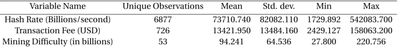
The data was then organized as a panel data set with observations reported for each of the 10 separate entities present in the data. Although each pool has 726 observations, many experience missing values either due to coming into existence in the midst of the data set or other, unknown reasons. Summary statistics for relevant variables have been provided below. Note that the total value of the transaction fee is the same for each pool on a given day and the difficulty is constant for all over the round. On the other hand, each pool has a unique hash rate for each day. This explains the discrepancy between the number of observations for the variables in Table 1.
Table 1:Summary Statistics of Data
Variable Name Unique Observations Mean Std. dev. Min Max
Hash Rate (Billions/second) 6877 73710.740 82082.110 1729.892 542083.700 Transaction Fee (USD) 726 13421.950 13484.160 2429.127 158063.200
Mining Difficulty (in billions) 53 94.241 64.536 27.800 220.756
Summary statistics of three primary variables: the hash rate of each individual pool (measured in billions of hashes per second), the total transaction fee received by all pools, and the mining difficulty as determined by the Bitcoin mining algorithm. Data spans the two year period between September 2014 and September 2016.
to compensate for variations over time, an accurate measure of available computational potential and innovation would have useful to include. The sparsity of the previously specified models is thus necessitated by the availability (or lack thereof) of data and may impact– through left out variable bias–the results presented in the following section.
VIII. R
ESULTS
The results we discovered were, at least initially, surprising and unintuitive. Rather than suggesting that pools are engaging in clear signs of collusion (adjusting their hash rates in the same direction) or are operating completely independently of one another (in which case we would expect insignificant peer effects), the regressions found a negative relationship between the hash rate of a particular pool and that of its competitors. In the tables that follow, we present the estimated coefficients and t statistics of the regressors, as well as the same information for the day fixed effects (since these values were also being analyzed to identify collusion). All regressions were performed using Stata, a statistical software program. Asterisks have been included to denote standard levels of confidence in statistical significant. A single asterisk signifies significance at a confidence level of 95%, two at 99%, and three at 99.9%.
We first ran the regression specified by equation 18, in which the hash rate of a particular pool is modeled as a function of the hash rate of peers and the total transaction fee earned from the prior day.
Table 2:Fixed Effects Without Lagged Hash Rates Observations: 6869
Variable Name Coefficient T Statistic Standard Error
ln(hashr ateother s)t,d -2.957 °4.810§§§ .614
ln(tr ans f ee)t°1 .418 3.880§§§ .108
Day=2 -.062 -1.350 .018
Day=3 -.081 -1.654 .028
Day=4 -.054 -1.193 .021
Day=5 -.010 -.292 .020
Day=6 -.075 -1.674 .026
Day=7 .083 -1.711 .017
Day=8 -.174 °3.735§§§ .022
Day=9 -.13 °2.88§§ .041
Day=10 -.115 °2.311§ .025
Day=11 -.174 °3.688§§§ .025
Day=12 -.112 °2.482§ .023
Day=13 -.146 °3.020§§ .024
Day=14 -.262 °4.681§§§ .040
Day=15 -.096 -.750 .091
Results of running the regression specified in equation 18. The natural log of the hashrate was included as the dependent variable. The hashrate of others and lag of the total transaction fee were independent variables. The day variables included in the table represent fixed effects.
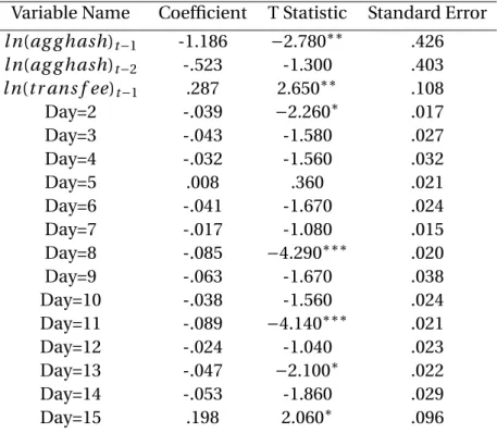
We next performed the regression specified by equation 19. Recall that this modeled the hash rate of a particular pool as a function of the lagged aggregate hash rates in the the prior two rounds and the transaction fee paid out in the previous period.
Table 3:Fixed Effects With Lagged Hash Rates Observations: 6869
Variable Name Coefficient T Statistic Standard Error
ln(ag g hash)t°1 -1.186 °2.780§§ .426
ln(ag g hash)t°2 -.523 -1.300 .403
ln(tr ans f ee)t°1 .287 2.650§§ .108
Day=2 -.039 °2.260§ .017
Day=3 -.043 -1.580 .027
Day=4 -.032 -1.560 .032
Day=5 .008 .360 .021
Day=6 -.041 -1.670 .024
Day=7 -.017 -1.080 .015
Day=8 -.085 °4.290§§§ .020
Day=9 -.063 -1.670 .038
Day=10 -.038 -1.560 .024
Day=11 -.089 °4.140§§§ .021
Day=12 -.024 -1.040 .023
Day=13 -.047 °2.100§ .022
Day=14 -.053 -1.860 .029
Day=15 .198 2.060§ .096
Results of the regression specified in equation 19. The natural log of the hashrate is the dependent variable. Two lags of the aggregate hashrate and a single lag of the transaction fee serve as the regressors. The day values specified correspond to fixed effects.
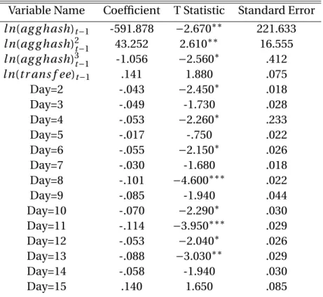
predominately base their decisions on only the previous period.
Table 4:Fixed Effects With Non-linear Lags Observations: 6621
Variable Name Coefficient T Statistic Standard Error
ln(ag g hash)t°1 -591.878 °2.670§§ 221.633
ln(ag g hash)2t°1 43.252 2.610§§ 16.555
ln(ag g hash)3t°1 -1.056 °2.560§ .412
ln(tr ans f ee)t°1 .141 1.880 .075
Day=2 -.043 °2.450§ .018
Day=3 -.049 -1.730 .028
Day=4 -.053 °2.260§ .233
Day=5 -.017 -.750 .022
Day=6 -.055 °2.150§ .026
Day=7 -.030 -1.680 .018
Day=8 -.101 °4.600§§§ .022
Day=9 -.085 -1.940 .044
Day=10 -.070 °2.290§ .030
Day=11 -.114 °3.950§§§ .029
Day=12 -.053 °2.040§ .026
Day=13 -.088 °3.030§§ .029
Day=14 -.058 -1.940 .030
Day=15 .140 1.650 .085
Results of the regression specified in equation 20. Natural log of the hash rate is the dependent variable while linear, quadratic, and cubic functions of hash rate lags and the transaction fee are the regressors.
negative fixed effects.
In totality, the regression results yielded surprising and somewhat contradictory indi-cations. While the day fixed effects would serve as evidence that pools are behaving in a collusive manner (since they appear to reduce their hash rate as the round proceeds), the negative relationship between a particular pools hash rate and that of its competitors suggests the opposite is true. Though we can’t dismiss the possibility that the benefits of collusion are being ignored in favor of ruthless competition, we now propose two alternate explanations that would explain the reported results.
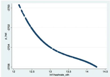
Figure 9:Non-Linear Relationship between pool’s hash rate and that of competitors
According to the regression results, the relationship between the hash rate of a particular pool and its competitors is characterized by a non-linear relationship. This suggests the effect of competitors altering their hash rates on a given pool’s hash rate will vary depending on the current level of the aggregate hash rate.
in unison, the outcome could imply pools are effectively "trading off" profitable rounds. In such a scenario, other pulls would reduce their hash rates to allow one (or perhaps a subset of all pools) to experience a more prosperous round. Once a given round ends, another pool would then swap into the desired role. While the implementation of this strategy would likely require more explicit communication between pools, it would explain the negative relationship discovered in the data.
be greater (pools share profits according to the share of computational power provided). An-other possibility involves the self-regulation that has been described previously. If a pool were to acquire a 51% market share, the entire blockchain would effectively be compromised since the pool could add erroneous blocks and edit the history of the ledger. As this is of grave concern to miners, they could intentionally be leaving a pool that becomes too concentrated. However, this explanation warrants a caveat. Since the most concentrated pool currently accounts for roughly a fifth of all hashing, reaching the 51% level is not a realistic feat for any pool in the near future.
As a final note, observe the final explanation, and the results in general, suggest there are constraints on the total amount of hashing that can occur in the market since a tradeoff appears to occur between competing pools. While one could, in theory, argue in favor of virtually unconstrained conditions–since pools have the ability to acquire a greater amount of computational resources and continually update their existing material–such an assertion is unrealistic. As was expressed in the theoretical model, adding to the stock of computational power will increase costs in the form of electricity bills and eventually render the mining activity profitable. Further constraints may include the slowing introduction of new min-ers (since profits are heavily dispmin-ersed throughout pools) and diminishing computational innovation realized in recent years.
IX. C
ONCLUSION
The theoretical model we constructed incorporated game theoretic elements in order to capture the interdependent relationship between pools. In the repeated game structure defined, we allowed the level of capital of a given pool to be directly related to its ability to successful include a block in the blockchain. By defining corresponding utility and value functions, we were able to compute closed form solutions for the utility obtained over the entire mining duration. These expressions then allowed us to determine which strategies served as subgame perfect Nash equilibriums through the utilization of the one-shot devia-tion principle. While this simple model proved sufficient for our purposes, it is worth noting the shortcomings and aspects in need of improvement. Further work could seek to the add the following enhancements: allow for an arbitrary number of pools, account for additional factors (transaction fees, desire to avoid too much concentration, etc.), along with a variety of others.
[1] Susan Athey, Ivo Parashkevov, Vishnu Sarukkai, and Jing Xia. Bitcoin pricing, adoption, and usage: Theory and evidence. 2016.
[2] Miguel A Fonseca and Hans-Theo Normann. Explicit vs. tacit collusionâ ˘AˇTthe impact of communication in oligopoly experiments. European Economic Review, 56(8):1759–1772, 2012.
[3] Armando Gomes. Multilateral contracting with externalities.Econometrica, 73(4):1329– 1350, 2005.
[4] Hanna Halaburda and Miklos Sarvary.Beyond Bitcoin: The Economics of Digital Curren-cies. Palgrave Macmillan US, 2016.
[5] Johannes Hörner. A perpetual race to stay ahead. The Review of Economic Studies, 71(4):1065–1088, 2004.
[6] Sober Mall. Foreign direct investment inflows in pakistan: A time series analysis with autoregressive distributive lag (ardl) approach. International Journal of Computer Appli-cations, 78(5), 2013.
[7] Charles F Manski. Identification of endogenous social effects: The reflection problem.
[8] Eric Maskin and Jean Tirole. Markov perfect equilibrium: I. observable actions.Journal of Economic Theory, 100(2):191–219, 2001.