Uncertainty in the Small and in the Large
∗
Wenfeng Qiu
†David S. Ahn
‡§November 10, 2020
[Most Recent Version]
Abstract
Most decisions are observed in isolation without direct measurement of correlation in beliefs across state spaces or complementarity in tastes across prize spaces. We introduce a novel model with two decision problems with distinct states and prizes, which we call small worlds, without observation of bets that are contingent on the realization of both worlds. We provide a characterization of subjective expected utility, where choices are made as if there is a joint distribution over the product of the state spaces and a joint utility index over pairs of prizes from both prize spaces. Turning to the identification problem, we show that the joint utility index over pairs of prizes and the marginal belief over each small world is identified, but the uniqueness of the joint distribution is more subtle. If the utility index is separable across prize spaces, then the correlation across state spaces is unidentified; but if there is any complementarity across prizes, then the joint distribution is exactly identified. We apply our analysis to provide behavioral foundations for independence of the distribution across state spaces. Finally, we generalize the model to allow for ambiguity about correlations.
∗We thank Haluk Ergin, Larry Karp, Chris Shannon and seminar participants at University of California,
Berkeley for helpful feedback.
†Department of Agricultural and Resource Economics, University of California, Berkeley, 714 University
Hall, Berkeley, CA 94720-3310. Email: wqiu03@berkeley.edu
‡Department of Economics, University of California, Berkeley, 530 Evans Hall, Berkeley, CA 94720-3880.
Email: dahn@econ.berkeley.edu
§Olin Business School, Washington University in St. Louis, Campus Box 1133, One Brookings Drive, St.
1
Introduction
Many environments involve multiple separate but possibly complementary choices across dif-ferent varieties of contingencies and outcomes. For example, a newly hired worker must enroll in a sponsored health insurance plan. Her choice reveals information about the employee’s beliefs about her health care needs, like requiring hospitalization. The same employee may also own private life insurance, revealing some information about her belief that she will die prematurely. The states that are relevant for these two decisions, such as a hospitaliza-tion that triggers a health insurance claim or an early death that triggers a life insurance claim, seem clearly correlated. At the same time, these decisions are empirically observed in isolation and without instruments to measure beliefs about the correlation. Theories of decision-making like subjective expected utility typically assume preferences for bets on all joint events are observed by the analyst. In this example, this would require a complicated insurance policy that pays only in the case of hospitalization without death. This paper provides a model that takes the separation of decisions seriously while acknowledging pos-sible correlation in states or complementarity in outcomes across decisions. We keep these decisions formally detached from each other, that is, we do not assume the existence of com-plicated bets across domains. We ask what can be inferred about the grand joint problem from observations of choices in smaller problems.
In a famous discussion, Savage discusses the tension between two proverbs: First, the principle of “Look before you leap” suggests enumerating all contingencies and outcomes before making a decision as demanded in observing preferences over all acts in subjective expected utility. Indeed, when making insurance decisions considering correlations across policies seems like an important consideration. Second, the principle that “You can cross that bridge when you come to it” suggests only the immediately relevant details be consid-ered since modeling all possible contingencies seems practically impossible for the decision maker and analytically impossible for the analyst. Indeed, real-world insurance policies are purchased separately across risks. Savage ultimately concludes that expected utility theory is best applied to small worlds since “to cross one’s bridges when one comes to them means to attack relatively simple problems of decision by artificially confining attention to so small a world that the ‘Look before you leap’ principle can be applied there (Savage (1954, p. 16)).” This paper introduces a model that takes an intermediate perspective between small and large worlds. We take seriously that a small world is a set of states and outcomes that is complete in the sense that all bets that assign different outcomes across different states are considered. That is, within that world the decision maker looks at all describable bets before she leaps to a decision. So the agent chooses across a comprehensive menu of
health insurance policies and a comprehensive menu of life insurance policies. On the other hand, we also acknowledge that decision makers face multiple choices. We therefore consider multiple small worlds simultaneously. However, we also acknowledge that these choices are often made apart from each other. We therefore keep small worlds isolated in the model, in the sense that bets can only be contingent on the realization of of a single small world, but cannot depend on the joint realization of states across worlds. So while she can choose a health insurance plan and a life insurance policy, the agent does not choose a grand policy that covers across joint hospitalization and survival risks. Our main question is: What can be inferred about the grand world only from observations across multiple small worlds? This is a theoretically novel question, and we introduce a new framework for analysis to address it.
Formally, we introduce a novel variation of the classic framework by Anscombe and Aumann (1963) (AA) to consider two worlds (or decision problems), each with its own state space,SorT, and its own outcome space,XS orXT. We consider preferences over profiles of
acts over small worlds, in this case over objects like (fS, fT), where fS :S →XS is a bet on
the first small state space that returns prize fS(s) depending on what states realizes in the
first world, and where fT :T →XT is a similar bet that depends on the state of the second
world. However, each small world is isolated from the other. Bets can depend on one state space or the other, but cannot have joint contingencies. For example, a bet that pays off only if states∈Sand statet ∈T are jointly realized is disallowed. Depending on perspective, our model can be viewed as either an expansion or a restriction of standard models of subjective uncertainty. On one hand, we expand the original Anscombe–Aumann analysis of a small world since now preferences over the marginal act in one world can depend on the held position in the other world. Our model is more rich than an Anscombe–Aumann model for either small world. On the other hand, we restrict the original Anscombe–Aumann analysis of the grand world since now bets that depend on the entire grand state space are prohibited. Our model is more spare than the Ansombe–Aumann model for the large world. In keeping with the original development of Anscombe and Aumann, we will consider lotteries over acts. Our first result characterizes an appropriate version of subjective expected utility for this new environment. The original Anscombe–Aumann axioms, including some that invoke the randomization over acts, turn out to still characterize maximization of an expected utility index over some fixed subjective belief. In this case, the utility index is defined over the grand prize space, namely XS ×XT, and the subjective belief is a joint distribution over
the grand state space S×T. This shows that the hypothesis of subjective expected utility has the same testable restrictions whether only small worlds are observed in isolation or the grand problem is directly observed with preferences over complicated bets.
We next study the identification of the parameters of the representation. Since our model enriches the Anscombe–Aumann model over a small world, we naturally obtain at least that level of identification: The (marginal) belief on either small state space S or T is uniquely identified. However, many candidate joint distributions can share common marginals. We show that the precision of mixed moments like correlation is bang-bang. There are two possible cases. In one case, nothing beyond the marginals is known and any subjective belief with those marginals will represent the same behavior. In the other case, the entire subjective belief is known exactly. That is, there is no nontrivial partial identification here. Which case obtains depends on the structure of the utility index over joint prizes. If there is no interaction between the two prize spaces, that is, if the utility index is additively separable across XS and XT, then only the marginals and nothing else about the distribution can be
identified. However, if there is any interaction, that is, any incidence of complementarity or substitution, then the entire joint distribution on the large state space S ×T is exactly identified. As an application, we consider the special case where XS and XT are both sets
of money lotteries. Then additive separability is equivalent to risk neutrality over money. Then, if there are two spaces of assets whose returns can be invested, our main result shows that the correlation in these assets can be exactly identified if there is any diversification benefit implied by risk aversion, but otherwise a risk-neutral investor’s believed correlations are unidentified.
Taking advantage of the product structure in our model, we propose a characteriza-tion of statistical independence across small worlds. We introduce a primitive condicharacteriza-tion on preferences that guarantees a subjective expected utility representation with a statistically independent belief.
Finally, our model allows us to distinguish between ambiguity over the marginals and over the correlations. We proposed an axiom that requires the mixture independence to hold within the set of marginal certain acts, which contains the acts that yield deterministic pay-offs in one small world. This axiom can be universally combined with the existing ambiguity models to characterize no ambiguity over the marginal beliefs so all the ambiguity, if any, is about how the small worlds are correlated.
We are not the first to consider formal models of small worlds. In fact, the mentioned discussion in Savage’s book is one of the most quoted parts of the whole treatise. Chew and Sagi (2008) consider the problem of identifying small worlds from a larger world. In particular, they identify coarser sub-algebras of the state space where the decision maker (DM) maintains probabilistic sophistication. Their aim is quite different from ours. They use departures of expected utility to endogenize what is a small world. In contrast, we take the small worlds as given and arrive at what looks like a classical expected utility
representation over the grand state space.
A paper whose formal model is closer to ours is the work of Ergin and Gul (2009). They also use a product state space, but their aim is to identify issue preference, where the DM prefers to bet on one dimension rather than another. Like the prior reference, they also use departures from probabilistic sophistication to identify the issue preference. The resulting representation would violate a condition we require later, which is essentially indifference to which issue resolved. That is, their theory is designed to detect departures from reduction of compound lotteries, while our requires no such departures exist. Similarly, Nau (2006) also considered a product state space to study issue preference via non-reduction of compound lotteries as a model for ambiguity aversion. However, both these papers consider preferences over all acts on the product state space, and do not have separate prize spaces for each issue or constrain the measurability of bets across issues.1 So our objective, of identifying the subjective probability over the product space, is delivered via an immediate application of known theorems when all acts are compared by the DM.
1Ergin and Gul (2009) use a purely subjective model, in the sense that they use a Savage primitive and
2
Model
For simplicity, we consider two small worlds but almost all our results can be generalized to the case with an arbitrary finite number of worlds. We consider two finite state spaces S, T
with S = {s1, s2, ..., sN}, T = {t1, t2, ..., tM}. A complete description of the world specifies
the realizations of both S and T, so the grand state space is the product space S ×T. Each small state space has an accompanying outcome space XS or XT. We employ the
Anscombe–Aumann structure and assume each outcome space XS or XT is the family of
simple lotteries, that is, lotteries with finite support, over a deterministic prize space ZS or ZT. Then XS =4ZS and XT =4ZT.2 Let δz denote a degenerate lottery concentrated at
point z.
Let FS = (XS)S and FT = (XT)T. That is, FS is the set of Anscombe–Aumann acts
from state spaceS to mixture spaceXS, and similarlyFT is the set of all acts fromT toXT.
Each problem is a well-defined Anscombe–Aumann domain, but by itself either FS orFT is
an incomplete description of the DM’s total problem because it ignores the other choice. So we consider the space F = FS × FT. That is, the DM holds two positions, one small act fS :S→XS that determines the outcome inZS depending on the realization of state s∈S
and another similar small actfT :T →XT.
We emphasize thatF is not a standard model of subjective uncertainty in the tradition of Savage. The grand state space S×T is like a usual state space, albeit with some additional structure. The grand prize space isZS ×ZT. A standard Anscombe–Aumann model would
consider all acts from (grand) states to lotteries over (grand) consequences, that is, any function f :S×T → 4(ZS×ZT). Our domain is a strict subset of this standard model. It
includes only grand acts where the first prize [f(s, t)]S ∈XS depends only on the realization
of state s ∈ S, and similarly [f(s, t)]T depends only on t ∈ T. More formally, we consider
acts where each projection to a prize space is measurable with respect to the associated state space. This excludes bets where the prize in XS depend on state t, for example a step
function that returns one pair (zS, zT) at a fixed grand state (s, t) but returns another pair
of prizes (zS0, zT0 ) elsewhere at all (s0, t0) 6= (s, t). This is because our goal is to understand what characteristics of the DM can be identified from partial information about small worlds, where we only see variation small world by small world. We exclude bets that parlay both dimensions of the state space. The DM may have correlation in her beliefs acrossS andT or have complementarity in her utility across XS and XT, but these features are not measured
directly. Our question is what can be inferred when only behavior in separate small worlds is observed.
We not only consider preferences over acts, but over lotteries of acts. Let 4F denote the family of simple lotteries of F. A lottery that yields the act fk with probability αk for
k = 1,2, ..., K is denoted as Q=PK
k=1α
kfk ∈ 4F. Our basic primitive is a binary relation
over 4F. The enriched domain eases the analysis by considering comparisons like whether a fixed act (fS, fT) is preferred to a coin flip 12(fS0, f
0 T) + 1 2(f 00 S, f 00
T) over a better act (f
0
S, f
0
T)
and worse act (fS00, fT00). Such comparisons allow cardinal interpretation of the differences in utilities across acts. This is in the spirit of the original Anscombe–Aumann model, and has been recently applied by, for example, Seo (2009) to study ambiguity aversion and by Ergin and Sarver (2015) to study menu choice. We exploit the randomization in a manner similar to these papers, to calibrate cardinal differences across acts. Also like these papers, our aim is to characterize a utility index over pure acts F.
An actf ∈ F is constant iffS(s) is constant insandfT(t) is constant int. So a constant act consists of two lotteries, one lotterypS ∈ 4ZS over the prize realized in ZS and another
lotterypT ∈ 4ZT over the prize realized inZT. When it engenders no confusion, we will refer
to a constant act by these lotteries (pS, pT). We assume that the associated randomization
devices are statistically independent. This is actually less objective randomization than the full set of joint distributions over prizes that would be required for the standard Ancombe– Aumann model from S ×T to 4(ZS ×ZT). That is, we do not assume the existence of
a randomization device that can produce all correlation structures, but rather assume only a device that can independently randomize over ZS and over ZT. For a pair of marginal
distributions over ZS and over ZT, their product distribution over ZS ×ZT is denoted by
φ(pS, pT) =pS×pT ∈ 4Z and is defined in the standard manner for all (zS, zT)∈ZS×ZT
by:
[φ(pS, pT)](zS, zT) = [pS×pT](zS, zT) =pS(zS)·pT(zT).
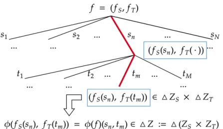
This construction can be extended pointwise from constant acts to arbitrary acts. A real-ization (s, t) of the grand state of the world induces lotteriesfS(s) and fT(t). So each state is associated with a product measure over ZS ×ZT and can be lifted as a function φ(f)
from S×T to φ(4ZS,4ZT), that is, from the grand state space to the family of product
distributions:
φ(f)(s, t) = (zS, zT) =pS(zS)×pT(zT).
We will assume that the DM evaluates a pair of lottery (pS, pT) ∈ 4ZS × 4ZT as if evaluating the lottery q = φ(pS, pT) ∈ 4Z. The pair of lotteries (pS, pT) can be viewed
Figure 1: Using the φ operator to reduce compound lotteries
reduction of this compounding lottery. We will state the assumption explicitly later as the Reduction Axiom and more details on this axiom in the uncertainty will be discussed.3 The Figure1 summarizes the discussion of the φ operator.
Our primary object of interest is a preferenceover the domainF. Like most models of choices under risk and uncertainty, it will be convenient to introducing mixture (i.e., convex combination) of lotteries and acts. The set of constant acts is identified with the space of product measures onZS×ZT. Unfortunately, the family of product measures is not convex.
For example, the half-half mixture of δ(zS,zT) and δ(zS0,z
0
T) is not in φ(4ZS× 4ZT) whenever
zS 6=zS0, zT 6=zT0 . Introducing lotteries over F convexifies the set of constant acts. One way
to see this is to observe that any degenerate distribution δzs,zt ∈ 4(ZS ×ZT) concentrated
on the grand prize (zs, zt) is a product measure. These mass points are the extrema of the simplex of lotteries and span 4(ZS ×ZT). So the convex hull of the family of product
measures over joint consequences is the entire4(ZS×ZT). The lack of convexity present an
immediate obstacle to analysis since almost all approaches to expected utility rely heavily on duality approaches that require convexity of domain. Without randomization, the set of constant acts is not even convex. This further explains our use of randomization in our domain4F: Not only is this randomization useful in the usual manner of calibrating sharper information about preferences, but here it is serves a more fundamental modeling purpose in closing the consequence space under mixtures.
In contrast to our work, almost all other models of subjective decision-making follow Anscombe and Aumann (1963) and consider a convex preference domain like ˜F = {f˜ :
S ×T → 4(ZS ×ZT)}, instead of F 4. Since ˜F contains all possible mappings from the
grand state space to the grand outcome space, we can call it a grand set of acts. As we will show, inferring the DM’s subjective belief over the grand state space from our domain 4F
is not always possible. This is in contrast to the standard model where observing preferences over ˜F identifies the entire belief. This difference in identification demonstrates that there is an important modeling distance between the set of grand acts ˜F and our domain of 4F.
4Following Anscombe and Aumann (1963), the mixture of two acts in ˜F can be identified as an act in
˜
3
Subjective Expected Utility with Unique Marginal
Beliefs
We first characterize an appropriate version of subjective expected utility for our framework. While many of the conditions will feel familiar from their application in standard Anscombe– Aumann domain, we caution that their interpretation is slightly different for our more limited domain.
Axiom 1. (Non-triviality)
There exists zT ∈ZT, zS, zS0 ∈ZS such thatδzS,zT δzS0,zT; there exists zS ∈ZS, zT, z
0
T ∈ZT
such that δzS,zT δzS,zT0 .
This assumption guarantees that each small world is relevant. It requires some strict preference for each dimension, so is a bit stronger than the standard assumption that requires only one incidence of strict preference somewhere.
Axiom 2. (Weak Order)
is complete and transitive.
This is a standard requirement for rational choice. Axiom 3. (Continuity)
For anyP QL, there existα, β ∈(0,1) such that αP+ (1−α)LQβP+ (1−β)L. We invoke a weak Archimedean version of continuity. The stronger topological notion of continuity is also implied by the representation, but Archimedean continuity is sufficient. Axiom 4. (Monotonicity)
If P(s, t)Q(s, t) (considered as constant acts) for all s, t, then P Q.
This condition guarantees that the utility for a grand prize pair (ZS, ZT) is invariant to
the state in which it is obtained. It also implies state-indepedence, that is, the utility for a prize is independent of the grand state in which it is earned.
Axiom 5. (Independence)
For all P, Q, L∈ 4F and allα∈(0,1), P Q ⇐⇒ αP + (1−α)LαQ+ (1−α)L. This standard condition maintains its interpretation in our model. It guarantees a linear representation over the space of lotteries over acts. So then there exists a linear expected-utility representationV :4F →Rover lotteries of acts. IfQ=PK
k=1αk(fSk, fTk) is a lottery
is V(Q) = PK
k=1α
kW(fk
S, fTk). Our main representation sharpens the structure of W, that
is, it is a formula for the value of degenerate lotteries over acts.
The final axiom is somewhat less common than the others in modern versions of the Anscombe–Aumann model, and invokes the structure of our expanded domain that includes lotteries over acts.
Axiom 6. (Reduction)
For any P, Q∈ 4F, φ(Q) =φ(P) =⇒ Q∼P.
This condition requires the DM to care only about the reduced distribution of prizes he would get in each state of the world. As an example, consider Q = 12f + 12g, P = l, where
f, g, lare all constant acts andf =δz1
S, δz1T, g =δzS2, δzT1, l =pS, δz1T withpS(z
1
S) = pS(z2S) = 12.
Clearly,P, Q are different elements in4F but φ(P) =φ(Q). The Reduction Axiom simply requires the DM to be indifferent betweenP, Q. The standard interpretation of this condition is tied to reduction of compound lotteries and attitudes towards the timing of uncertainty. A lottery over Anscombe-Aumann acts is a compound lottery: first, an act (fS, fT) is realized
from the lottery over acts, then second a state (s, t) is realized and a lottery φ(fS(s), fT(t))
over prizes is paid. Instead, suppose we first realized a state (s, t), then second draw a lottery over which act’s payoff is realized. The Reduction Axiom asserts the DM’s indifference between these two orders for realizing uncertainty.
So one reading of the following representatation theorem is to understand the force of the original Anscombe–Aumann axiom scheme when applied over a product of small worlds, rather than directly over all grand acts. The following result shows that these conditions remain sufficient for subjective expected utility. However, as we will explore in more detail in the sequel, there will be a gap between the uniqueness of the parameters across the two domains. That is, the analytic loss in the Anscombe–Aumann framework of considering only small worlds is not in the testable content of subjective expected utility, but rather in the sharpness of its implicit parameters.
Nearly all recent applications of the Anscombe–Aumann framework drop randomization over acts, so take no position on compounding. However, restrictions that are very similar to the reduction axiom appear in the original treatment by Anscombe and Aumann that explicitly considers lotteries over acts. That is, if S is a state space and X is a mixture space, then the original Anscombe–Aumann domain was actually 4(XS), even thogh most
modern treatments study preferences over XS. This is because in many applications, the
additional randomization provides no benefits because the relevant representation can be characterized and identified with the sparser domain. Here, the richness of randomized acts is crucial in obtaining our results.
Theorem 1. (Subjective Expected Utility with Unique Marginal Beliefs)
satisfies Axioms 1-6 if and only if it is represented byV (or equivalently, by (U, µ)), i.e.,
for Q=PK k=1α kfk with αk >0,PK k=1α k = 1, V(Q) = K X k=1 αk[X n,m µ(sn, tm)·U(φ(fSk(sn), fTk(tm)))] (1)
where µis a probability measure over S×T andU :4Z →R is an expected utility function,
i.e., U(q) =P
jq(z
j)·u(zj).
Moreover, uis nonconstant and unique up to positive affine transformation. The marginal
beliefs µS(sn) := P
mµ(sn, tm), µT(tm) :=
P
nµ(sn, tm) for any sn, tm are unique. 5
We briefly sketch the proof here. The Reduction Axiom allows us to construct a preference relation ˙overφ(4F) defined byφ(Q) ˙φ(P) if and only if QP. Next, we apply the von Neumann–Morgenstern Expected Utility Theorem for objective risk to the set of lotteries over constant acts 4(ZS×ZT) and identify the expected-utility function U : 4Z → R.
So the utility index over grand prizes is immediately revealed through the lotteries over constant acts. Note that without convexification this would not be possible, since F does not include all distributions over ZS ×ZT while 4F does contain all such lotteries. Now
define a mapping π : φ(4F) → RN M such that the nmth coordinate of π(φ(Q)) is given
by U(φ(Q)(sn, tm)). We verify that π(φ(4F)) is a convex subset of RN M.6 Next, define the binary relation R over π(φ(4F) by π(φ(Q))Rπ(φ(P)) if and only if φ(Q) ˙φ(P). We showRsatisfies the axioms required by the Mixture Space Theorem and thus obtain a linear representation. The Mononicity Axiom implies the weights of the linear representations are nonnegative and thus can be normalized as a belief µ.
A key difference in our representation theorem from the canonical Anscombe–Aumann representation is that the DM’s subjective belief over the grand state spaceS×T is possibly unidentified. Instead, only the marginal beliefs µS, µT are unique. The next section will
discuss the uniqueness of the subjective belief in some detail. However, it may be useful to briefly discuss here some of the geometry for the possibly non-identification. The proof proceeds by generating a linear function V on the span of π(φ(4F)). The key issue is that π(φ(4F)) may not span all of RN M. In that case, there are multiple linear extensions
of V from the span of π(φ(4F)) to RN M, and any of these extensions also represent the
same behavior. It turns out that the gap in the span can be tested with a condition on deterministic preferences, namely additive separability.
5That is, if (U, µ),(U0, µ0) both represents,µ
S =µ0S, µT =µ0T.
4
Additively Separable Preference and Unique Belief
In this section, we study the case where preferences over prizes Z are additively separable across ZS and ZT, i.e., the u of representation (1) is additively separable. One
interpre-tation for separability is the neutrality of complementarity and substitution. For example, in intertemporal consumption problems, the time separable preferences are widely used in economics if we view (zT, zS) as consumption streams for two periods. We will give two
distinct approaches to characterize the additively separable preference. The first is a direct approach, imposing restrictions on lotteries over constant acts and thus uncertainty does not play any role. In the second approach, we impose restrictions on conditional preferences, i.e., the preference over payoffs on one dimension conditional on the payoffs from the other dimension. Under additive separability, we show inferring the DM’s beliefs beyond their marginal beliefs is impossible.
4.1
Direct Characterization of Additive Separability
Our first characterization of the additive separable preference directly impose restrictions on preferences over objective risk, i.e., the preferences over lotteries over constant acts. Additive separability has a long tradition in the theory of measurement and we follow the treatment for expected utility theory by Fishburn (1982). Let Q ∈ 4F be a lottery over constant acts and thenφ(Q) can be viewed as a lottery in4Z. For any element zS ∈ZS, we
write φ(Q)S(zS) =
P
zT∈ZT φ(Q)(zS, zT). So φ(Q)S(zS) is the marginal probability that the
DM obtains prize pairs containing zS in the first dimension (and φ(Q)T(zT) can be defined
similarly). The main axiom in Fishburn (1982) requires the DM to be indifferent between two lotteries in 4Z if their marginal probabilities over ZS, ZT are the same, which is translated
to our context as follows.
Axiom 7. (Additive Separability)
Let P, Q ∈ 4F be lotteries over constant acts. If φ(P)S(zS) = φ(Q)S(zS) for all zS ∈ ZS
and φ(P)T(zT) =φ(Q)T(zT) for all zT ∈ZT, thenP ∼Q.
The Additive Separability Axiom requires that for a joint distribution on ZS ×ZT, its
marginal lotteries over the separate prize spaces ZS and ZT are sufficient statistics for the expected utility of that lottery. This indifference to the mixed moments characterizes additive separability across small prize spaces. In addition, when there is indifference to mixed moments of a lottery over the grand prize space, then the analyst has no approach to estimate the mixed moments of the subjective belief over the grand state space S×T. In fact, any subjective belief with the same marginals will generate the same betting behavior.
Theorem 2. (SEU with Additively Separable Utility)
satisfies Axioms 1-7 if and only if it is represented by V (or (U, µ)) as in (1) and u is
additively separable, that is, u(zj) = uS(zSj) +uT(zTj).
Moreover, suppose (uS, uT, µ) represents %. Then (u0S, u
0
T, µ
0) represents
% if and only
if:
1. u0S =auS+b and u0t =aut+b for fixed a >0 and b∈R, and
2. µ0S =µS and µ0T =µT
Suppose that the utility index U is additively separable, or equivalently that % satisfies the Additive Separability Axiom. Then the two dimensions of the index uS anduT are
iden-tified up to joint positive affine transformation and the beliefµis identified up to marginals. That is, the correlation structure of µ is completely unidentified and the analyst cannot discriminate between even perfect positive or negative correlation.
The intuition behind the lack of uniqueness in Theorem 2 about the uniqueness of µ
turns out to be straightforward. As we show in the proof, ifuis additively separable, then the representation (1) can be decomposed into two parts that each only depends on one dimen-sion. In other words, the whole decision problem can be decomposed into two independent sub-problems and therefore any correlation across S, T is irrelevant. This observation also motivates our second approach to characterizing additive separability, which appeals to these conditional preferences.
4.2
Conditional Preference and Additive Separability
For a fixed fS ∈ FS, we can define the restricted domain F | fS := {g ∈ F : gS(s) = fS(s) for all s∈S}. For a preferenceover4F, its restriction overF |fSis the conditional
preference, which is denoted asfS. There is clearly a natural isomorphism between F |fS
andFT and thus a conditional preferencefs induces a preference relation overFT. Similarly,
for a fixedfT ∈ FT, the restriction of overF |fT is the conditional preference fT, which
induces a preference relation over FS.
In general, if fS 6= gS, then the conditional preferences fS,gS over FT may diverge.
This simply reflects the interaction of the two worlds. A natural question arises is when these conditional preferences are the same for different fSs. It turns out that if the DM’s
preference over 4F is represented by a SEU representation (1), then these conditional preferences agree if and only if u is additively separable. That is, if preferences over bets on state space T are independent of the bets held on state space S, then preferences over joint prizes exhibit no interaction. The identical conditional preferences can be formally summarized as the following two axioms.
Axiom 8. (Identical Conditional Preferences S)
For any fS, gS ∈ FS, the marginal preferencesfS,gS overFT agree. Axiom 9. (Identical Conditional Preferences T)
For any fT, gT ∈ FT, the marginal preferences fT,gT over FS agree.
Theorem 3. (Conditional Preferences and Additive Separability Under SEU)
Suppose the preference over 4F is represented by SEU (1), then the following statements
are equivalent:
1. satisfies the Additive Separability Axiom.
2. u is additively separable as in Theorem 2.
3. satisfies the Identical Conditional Preference S.
4. satisfies the Identical Conditional Preference T.
The Theorem 3 provides an alternative characterization to the Theorem 2. The equiva-lence between the three axioms (under the SEU) are somehow surprising because the their interpretations are quite different. In particular, the Additive Separability Axiom directly imposes restrictions on the preferences without uncertainty. While the Identical Conditional PreferenceS (T) Axiom requires the DM’s preference over payoffs from one dimension to be unaffected by the background uncertainty in the other dimension.
4.3
Uniqueness of Belief
Theorem 2shows that if the preference is additively separable, then the belief µin the SEU representation can only be identified up to its marginalsµS, µT. It turns out the converse of
this statement is also true, i.e., if the preference isnot additively separable, then the beliefµ
in the SEU is unique. Note that any complementarity is sufficient, so the two theorems cover all cases. That is, the only possible cases are either that only the marginals are identified and nothing else, or that the entire distribution is identified. There are no intermediate partial identification regions.
Theorem 4. (Uniqueness of Belief )
Suppose the preference over 4F has a SEU representation (1). Then the belief µ is
unique if is not additively separable.
To sketch the proof of Theorem 4, we introduce some additional notations. For any
s ∈ S, t ∈ T, we define Fst =: {f ∈ F : f
s, t0, t006=t}. An actf inFst withf
S(s) =pS, fS(s0) = p0S for all s0 6=s, fT(t) =pT, fT(t0) = p0T for all t0 6=t can be rewritten as ((pS, p0S)s,(pT, p0T)t) for convenience. By the SEU
repre-sentation (U, µ), over the restricted domain Fst ⊂ F is evaluated by: V(f) =µ(s, t)U(φ(pS, pT)) +µ(S\s, t)U(φ(p0S, pT)) +µ(s, T \t)U(φ(pS, pT0 )) +µ(S\s, T \t)U(φ(p 0 S, p 0 T))
Following a similar strategy as in the proof for Theorem 1, we can define a preference relationR over π(φ(4Fst) such that π(φ(Q))Rπ(φ(P)) if and only if QP for anyP, Q∈
4Fst. Note that each element π(φ(Q))∈ π(φ(4Fst) can be identified as an element in
R4 because by constructionπnm(φ(Q)) =πij(φ(Q)) if s
n, si ∈S\s, tm, tj ∈T \t. For example,
for the f above, π(φ(f)) can be identified by
(U(φ(pS, pT)), U(φ(p0S, pT)), U(φ(pS, p0T)), U(φ(p 0 S, p 0 T))∈R 4
ThusV is a linear function representing a preference relationR overπ(φ(4Fst)7, which
is identified as a subset U of R4. If we can show the linear representationV above is unique
then we are done, since µ(s, t) is then unique for arbitrary s, t. By Lemma 1, it is sufficient to show that U is convex, contains the zero vector, and spans R4. The convexity is free because we convexified the domain. Because U in the SEU representation is unique up to positive affine transformation, we can choose a U such that U contains the zero vector in R4 by considering a constant act and shifting uniformly to the origin. It remains to prove U spans R4, and the details of this proof is in the appendix.
4.4
Application: Monetary Payoffs
In this part, we consider the special but important case where the outcome spaces are monetary payoffs, that is, where ZS = ZT = R. This can be interpreted as investment
returns from two different assets, where the return of each asset depends on the realization of the state of world in its dimension. Then the DM only cares about the total monetary payoff summed across the two investments. We therefore specialize the main representation (1) so that there existsv :R→R such that u(zS, zT) =v(zS+zT) for all zS ∈R, zT ∈R.
Letφ∗ :4R×4R→ 4Rbe theconvolutionoperator, i.e.,φ∗(pS, pT)(z) = P
zT+zS=zpS(zS)·
pT(zT). We can apply the convolution operator toQ= PK k=1α kfk ∈ 4F as follows: φ∗(Q)(s, t) = K X k=1 αkφ∗(fSk(s), fTk(t))
Axiom 10. (Monetary Payoffs)
• For any P, Q∈ 4F, φ∗(Q) =φ∗(P) =⇒ Q∼P. • zS+zT > z0S+z 0 T =⇒ (δzS, δzT)(δz0S, δz 0 T)
The Monetary Payoffs axiom has two parts. The first part requires that the DM only cares about the total monetary payoffs and this part is stronger than the Reduction axiom because φ(P) =φ(Q) =⇒ φ∗(P) =φ∗(Q). The second part of the axiom simply says more money is strictly better and it is clear the second part implies the Non-triviality axiom.
Theorem 5. (Monetary SEU)
satisfies Axioms 2-5,10 if and only if it has a monetary SEU representation V (or
equiv-alently, (U, µ)), i.e., for Q=PK
k=1αkfk with αk>0, PK k=1αk= 1, V(Q) = K X k=1 αk[X n,m µ(sn, tm)·U(φ∗(fSk(sn), fTk(tm)))] (2)
, where µ is a probability measure over S ×T and U : 4R → R is an expected utility
function, i.e., U(q) = P
jq(z
j)·v(zj) and v is strictly increasing and unique up to positive
affine transformation. The marginal beliefs µS, µT are unique.
We say v is risk neutral if for any x, y ∈ R, 12v(x) + 21v(y) = v(12x+ 12y). One can easily show thatv is risk-neutral if and only ifu is additively separable. Thus we can apply Theorem 4 here and obtain the following proposition.
Proposition 1. (Belief Identification and Risk Neutrality)
Suppose is represented by V as (2), then
• v is risk neutral =⇒ if µ0S =µS, µ0T =µT, then (U, µ0) also represents .
• v is not risk neutral =⇒ µis unique.
To get the intuition behind the second part of Proposition 1, we use an investment example to demonstrate how the belief can be identified when the DM is risk averse. Suppose the DM has a monetary SEU representation and her utility over money isv :R→R. Assume
v is strictly concave, i.e., the DM is risk averse. The DM is considering investments in a stock and a bond. LetS ={H, L}, T ={h, l}, whereH/Ldenotes the high/low stock price, and h/l denotes the high/low bond price.
By Theorem 1, the marginal beliefs must be unique so we let α = µS(H) =: µ(H, h) + µ(H, l), β = µT(h) =: µ(H, h) +µ(L, h) and take α, β as given. We assume α ∈ (0,1), β ∈
(0,1), α+β < 1 for convenience. Let γ =µ(H, h) and it is clear that if we can identify γ, then µover S×T will be identified. We propose a way to recover γ.
Consider an act f such that for any∈R,
fS(H) = 1 2; fS(L) = − 1 2 fT(h) = 1 2; fT(l) = − 1 2
Call f “act” and the act can be interpreted as long positions in both stock and bond. The payoff matrix is given as follows:
Bond h l Stock H 1 2 + 1 2 1 2 -1 2 L −1 2 + 1 2 − 1 2 -1 2
The DM evaluates the act by:
V() = γv() + (α+β−2γ)v(0) + (1−α−β+γ)v(−)
When = 0, the DM receives $0 with certainty. Consider the DM’s choice between the risky act and receiving $0 with certainty. In particular, she prefers the certainty prize $0 if and only if
V(0)≥V() ⇐⇒ v(0)≥ γ
1−α−β+ 2γv() +
1−α−β+γ
1−α−β+ 2γv(−)
The RHS is the expected utility from a lottery that yields with probability 1−α−γβ+2γ and yields − otherwise. The expected return from the RHS lottery is equal to −1−α−β+γ
1−α−β+2γ
and the expected return is positive if and only if < 0. In order to make the risk-averse DM to be indifferent, the expected return from the RHS lottery must be large enough to compensate the DM. Let’s assume there exists ∗ <0 such that the act ∗ ∼$0 so $0 is the certainty equivalence for the act∗. It followsγ can be solved by the equationV(0) =V(∗), which establishes the uniqueness of γ and µ.
The argument above does not work for the case when v is risk neutral. When the DM is risk neutral, she only cares about the expected return of the RHS lottery. Note that the expected return−11−−αα−−ββ+2+γγ 6= 0 whenever 6= 0. Thus we cannot find non zero∗ such that $0 is the certainty equivalence for the act ∗.
5
Behavioral Characterization of Statistical
Indepen-dence
As an application of our framework, we study how to test whether the DM’s beliefs are correlated across state spaces. Note that independence of belief is a weaker hypothesis than additive separability, since there might be complementarity in the utility index over joint prizes without correlation in subjective belief over grand states. We provide behavioral conditions that are necessary and sufficient for representation by an independent measure over S×T.
An event in S is a subset ES ⊆ S := ∪s∈ES,t∈T{(s, t)} and an event in T is similarly
defined. Given the product state space S×T and the SEU representation, the events in S
and T might be statistically independent according to the DM’s subjective belief µ. That is, µ is the product measure generated by its marginals µS, µT. We are interested in the
behavioral implications of the statistically independent belief µ, i.e., observable restrictions over the DM’s preference .
Definition 1. (Statistically Independent Belief)
A belief (probability measure) µ over S ×T is called statistically independent if for any
s∈S, t∈T, µ(s, t) =µS(s)·µT(t), where µS, µT are the marginal beliefs.
For any s∈S and f, g ∈ F, we definefsg =hsuch that hS(s) = fS(s), hS(s0) =gS(s0)
for all s0 6=s and hT =gT. In other words, f sg =h agrees with g except its prize in the S dimension is the same as f if s is realized. Similarly, for any t ∈T, we define ftg =h
such that hT(t) = fT(t), hT(t0) = gT(t0) for all t0 =6 t and hS = gS. We introduce a subset
of the acts F that leads to payoffs with certainty in S or T dimension, which we call the marginally certain acts.
Definition 2. (Marginally Certain Acts)
Let F | S := {f ∈ F : fS(s) = fS(s0) for all s ∈ S} and F | T := {f ∈ F : fT(t) = fT(t0) for all t∈T}. We call F |S the S−certain acts and F |T the T−certain acts.
We can now introduce the behavioral conditions of interest. Axiom 11. (Statistical Independence S)
For any s ∈ S and f, g, f0, g0 ∈ F | S such that fT = gT, fT0 = g
0
T, if f 6∼ g and f sg ∼ αf + (1−α)g for some α∈[0,1], thenf0sg0 ∼αf0+ (1−α)g0.
Axiom 12. (Statistical Independence T)
For any t ∈ T and f, g, f0, g0 ∈ F | T such that fS = gS, fS0 = g
0
S, if f 6∼ g and f tg ∼ αf + (1−α)g for some α∈[0,1], thenf0tg0 ∼αf0+ (1−α)g0.
We will explain the axioms in more detail after we introduce the theorem. Theorem 6. (SEU with Statistically Independent Beliefs)
Suppose has an SEU representation (1), then the following are equivalent:
1. has an SEU representation (1) with a statistically independent µ.
2. satisfies the Statistical Independence S Axiom.
3. satisfies the Statistical Independence T Axiom.
The first statement of Theorem 6 asserts the existence of a statistically independent µ, but says nothing about its uniqueness and allows for the possibility of other representing measures. Ifµin the SEU is unique, then it must be statistically independent. If the beliefs are not unique, by Theorem 4, the product measure µ that is generated by its marginals will also rationalize the preference. Therefore, the Statistical Independence S, T axioms are logicaly weaker than assuming that the preference is additively separable.
We take the Statistical IndependenceS axiom to deliver the intuition behind Theorem6
since the intuition behind Statistical Independence T axiom is symmetric. For simplicity, assume the small state spaces are binary S = {s1, s2}, T ={t1, t2}. We further assume the
small prize spaces are binary ZS = {0,1}, ZT = {$50,$100}, e.g., in the S dimension the
prizes are chocolates and in the T dimension the prizes are dollars.
Consider constant acts f = (1,$50), g = (0,$50) and assume more is better, i.e., g f. Then h = f s1 g will deliver f if s1 ∈ S is realized and deliver g otherwise. Under SEU,
the DM does not care whether the probability is subjective or objective. Thus she must be indifferent betweenhand an objective lottery that yieldsf withµS(s1) andgwith 1−µS(s1).
SoµS(s1) is a good candidate for α in the axiom.
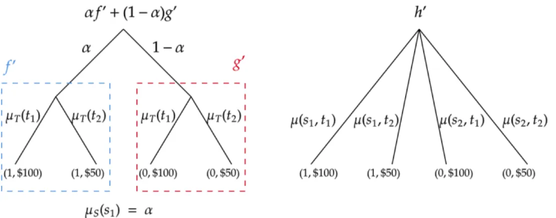
Next we consider acts f0, g0 and h0 =f0s1 g
0 as follows (see Figure 2):
fS0 = 1; fT0(t1) = $50 fT0(t2) = $100
gS0 = 0; g0T(t1) = $50 g0T(t2) = $100
h0S(s1) = 1 h0S(s2) = 0; h0T(t1) = $50 h0T(t2) = $100
In Figure 2, the DM’s evaluation of h0 is described by the right panel and her evaluation of αf0+ (1−α)g0 is described by the left panel. In particular, αf0+ (1−α)g0 is a two stage lottery and its probability α,1−α in the first stage is objective. In other words, we use of our objective randomization device, which is statistically independent of the states of the world, to mimic the uncertainty in the S dimension. If µ is statistically independent, then the DM will be indifferent betweenαf0+ (1−α)g0 and h0 since she does not care whether the
Figure 2: Intuition for Statistical Independence
probability in the first stage is objective or subjective. We believe this characterization will not work with Savage style acts because the objective randomization device is not assumed.
6
Ambiguity over Marginals and Correlations
Ellsberg (1961) famously suggested a thought experiment where many people would prefer to bet on a box with objective odds than either color in a box whose proportions are ambiguous. A huge literature has been developed to model ambiguity. Recent experimental evidence by Epstein and Halevy (2019) suggests the importance of modeling ambiguity about correlation. In this section, we illustrate how our framework can be used to distinguish between ambiguity over marginals and over correlations. We propose a universal axiom that can be imposed to a wide range of existing ambiguity aversion models to excluding ambiguities within each small world.
Axiom 13. (Marginal Certainty Independence)
For all f, g, h∈ F |S and α∈(0,1), f g ⇐⇒ αf + (1−α)hαg+ (1−α)h; For all f, g, h∈ F |T and α∈(0,1), f g ⇐⇒ αf + (1−α)hαg+ (1−α)h;
The Marginal Certainty Independence (MCI) axiom requires the Independence axiom to hold within the set of S−certain acts and the set of T−certain acts. If we weaken the Independence axiom with the MCI axiom, then we can obtain the SEU representations on
4(F |S),4(F |T) respectively, which suggests that the DM have unique marginal beliefs overS, T. In other words, this axiom implies there is no ambiguity over the marginal beliefs and all the ambiguity, if any, must be about the correlation between S, T.
For all the propositions below, when we say the expected utility function U : 4Z → R
is nontrivial, we mean its utility index u:Z →R is nontrivial in both dimensions. Proposition 2. (Maxmin Model with MCI)
over 4F is said to have a Maxmin Expected Utility (MEU) representation if there exists
a closed, convex set C ⊆ 4(S×T) and a non trivial expected utility U :4Z →R such that
is represented by V, V(Q) = min µ∈C X s,t µ(s, t)·U( K X k=1 αk[φ(fSk(s), fTk(t))])
Suppose has a MEU representation, then satisfies MCI if and only if for any µ, µ0 ∈ C,
µS =µ0S, µT =µ0T.
The MEU model was developed by Gilboa and Schmeidler (1989) to explain ambiguity aversion. In the MEU model, the DM has a set of priors over the states of the world and evaluates a prospect using the prior that gives the worst payoff. Under MCI, the set of priors must agree on their marginals.
Proposition 3. (Choquet Model with MCI)
over4F is said to have a Choquet Expected Utility (CEU) representation if there exists a
capacityνoverS×T and a nontrivial expected utilityU :4Z →Rsuch thatis represented
by V (where the integral is the Choquet integral),
V(Q) = Z S×T U( K X k=1 αk[φ(fSk(s), fTk(t))]) dν(s, t)
Suppose has a Choquet representation, then satisfies MCI if and only if the marginals
of the capacity νS, νT are probability measures.
In the CEU model by Schmeidler (1989), the DM’s belief over the states of the world is described by a capacity, in instead of a probability. The capacity is not necessarily additive and can be used to model behaviors in Ellsberg’s paradox. Under MCI, the marginal capacity inS, T must be additive, i.e., a probability.
Proposition 4. (Smooth Model with MCI)
over 4F is said to have a smooth ambiguity aversion representation if there exists a
probability measure M over 4(S×T), a nontrivial expected utility U : 4Z → R and a
strictly concave second order utility function Φ :R→R such that is represented by V,
V(Q) = K X k=1 αk Z 4(S×T) Φ[X s,t µ(s, t)·U(φ(fSk(s), fTk(t)))] dM(µ)
Suppose has a smooth representation, then satisfies the MCI if and only if for any
µ, µ0 ∈supp(M), µS =µ0S, µT =µ0T.
In the smooth model, the DM has a second order belief, i.e., a probability distributionM
over beliefs µs over the states of the world. Given M, each act will be a compound lottery. The smooth ambiguity model does not assume the DM evaluates the compound lotteries in the same way as their one shot reductions 8. In particular, the concavity of Φ explains
ambiguity aversion behavior. The smooth model was proposed by Klibanoff, Marinacci, and Mukerji (2005). Similar models with different preference domains were characterized in Nau (2006), Ergin and Gul (2009) and Seo (2009). Among these models, the domain used by Seo (2009) was closest to ours as the preference is defined on lotteries over acts. Under MCI, the beliefs in the support of the second order belief M must agree on their marginals.
8The idea of modeling ambiguity aversion by relaxing the reduction of compounding lotteries first
References
Anscombe, Francis J. and Robert J. Aumann (1963). “A definition of subjective probability”.
The Annals of Mathematical Statistics.
Chew, Soo Hong and Jacob S. Sagi (2008). “Small worlds: Modeling attitudes toward sources of uncertainty”. Journal of Economic Theory.
Ellsberg, Daniel (1961). “Risk, ambiguity, and the Savage axioms”. The Quarterly Journal
of Economics.
Epstein, Larry G and Yoram Halevy (2019). “Ambiguous Correlation”. The Review of
Eco-nomic Studies.
Ergin, Haluk and Faruk Gul (2009). “A theory of subjective compound lotteries”. Journal
of Economic Theory.
Ergin, Haluk and Todd Sarver (2015). “Hidden actions and preferences for timing of resolu-tion of uncertainty: Timing of resoluresolu-tion of uncertainty”. Theoretical Economics.
Fishburn, Peter C. (1982). The Foundations of Expected Utility.Kluwer Boston, Inc.
Gilboa, Itzhak and David Schmeidler (1989). “Maxmin expected utility with non-unique prior”. Journal of Mathematical Economics.
Klibanoff, Peter, Massimo Marinacci, and Sujoy Mukerji (2005). “A smooth model of decision making under ambiguity”. Econometrica.
Kreps, David (1988). Notes on the Theory of Choice. Westview press.
Nau, Robert F. (2006). “Uncertainty Aversion with Second-Order Utilities and Probabili-ties”. Management Science.
Savage, Leonard J. (1954). The Foundations of Statistics. John Wiley & Sons.
Schmeidler, David (1989). “Subjective Probability and Expected Utility without Additivity”.
Econometrica.
Segal, Uzi (1987). “The Ellsberg paradox and risk aversion: An anticipated utility approach”.
International Economic Review.
— (1990). “Two-Stage Lotteries without the Reduction Axiom”.Econometrica. Seo, Kyoungwon (2009). “Ambiguity and Second-Order Belief”. Econometrica.
7
Appendix
7.1
Technical Lemmas
Lemma 1. (Uniqueness of Linear Function)
Let R be a preference relation over U ⊆RK, where U is a convex set containing the origin
0K ∈
RK and span(U) =RK. Suppose there exists µ∈RK withPKk=1µ
k = 1 such that R is
represented by V: for any r∈RK,
V(r) = K X k=1 µk·rk =µr Then µ is unique.
Proof. Suppose µis not unique, so we have anotherµ0 6=µand PK
k=1µ
0k= 1 such that R is
represented by V0(r) = µ0r.
We first claim there exists x ∈ RK such that µx = 0 but µ0x 6= 0. To prove the
claim, suppose it is not true. So for any x ∈ RK, µx = 0 =⇒ µ0x 6= 0. For any
i, j ∈ {1,2, ..., K}, i 6= j, consider xij ∈ RK such that xiij = µj, x j
ij = −µi, xkij = 0 for all k 6=i, j. Clearly,µxij = 0 and this impliesµ0xij, which impliesµ0iµj =µ0jµi. For anyµi = 0,
we can choose someµj 6= 0 to obtain µ0i = 0. Symmetrically, for anyµ0i = 0, we can choose
some µ0j 6= 0 to obtain µi = 0. We hence conclude for anyk, µk = 0 ⇐⇒ µ0k = 0. For the
rest of nonzero µks, µ0iµj =µ0jµi and the definition of µ, µ0 together implies µk =µ0k. But all these yields µ=µ0, a contradiction.
Let {b1, b2, ..., bK} ⊂ U be a basis of RK. The existence of such as basis is guaranteed sincespan(U) = RK. Consider the vectory= 1
K+1
PK
k=1bk, which is the convex combination
of {b1, b2, ..., bK} and 0K with equal weights. Note that y ∈ U since U is a convex set
containing 0K. We claim there exists ∈ (0,1] such that (1 − )y + x ∈ U. To see
this, suppose x = PK k=1α kb k. Let PK k=1 | α k |= α and we pick = 1 α(K+1)+1. Then (1− )y+ x = PK k=1βkbk, where βk = α+α k
α(K+1)+1. Note that for all k, β
k ≥ 0 by the
definition of α. Also note that PK
k=1β k = αK+PKk=1αk α(K+1)+1 ≤ αK+PK k=1|αk| α(K+1)+1 = α(K+1) α(K+1)+1 < 0. So
(1−)y+x is a convex combination of {b1, b2, ..., bK} and 0K and thus belong to U.
Finally, since µ((1−)y+x)) = (1−)µy+µx=µy, y is indifferent to (1−)y+x
according to µ. But (1−)µ0y+µ0x=6 µ0y, soy is not indifferent to (1−)y+x according toµ0. This yields a contradiction to µ, µ0 both representing R.
Lemma 2. (Violations of Additive Separability)
there exists zS, z0S ∈ ZS, zT, zT0 ∈ZT such that P = 12(zS, zT) +12(z0S, z0T)6∼ Q= 12(z 0 S, zT) + 1 2(zS, z 0 T).
Proof. Suppose the statement is not true, then the Axiom 7* in the Theorem 2 of Chapter
6 in Fishburn (1982) holds. But in our context, this axiom is equivalent to the Additive Separability Axiom.
7.2
Proof of Theorem
1
Proof. The necessity part is straightforward to verify and we prove the sufficiency. Note
that the reduction axiom allows us to define a preference relation ˙ over φ(4F) such that
φ(Q) ˙φ(P) if and only ifQP. To save notation, we will useover φ(4F) instead of ˙. We first restrict on constant lotteries φ(Q), i.e., φ(Q)(s, t) = φ(Q)(s0, t0) for all s, t (it is clear that this requirement is satisfied if and only if Q is a lottery over constant acts). By Lemma 1, these lotteries will be 4Z. The restricted on 4Z satisfies weak order, continuity and independence axioms, which are required for the Expected Utility Theorem (e.g., see Kreps (1988)). Sooverq∈ 4Zis represented byU, whereU(q) =P
jq(z
j)·u(zj)
and u is unique up to positive affine transformation. Fix this u. By the Non-triviality and Monotonicity Axiom, u cannot be constant valued and so as U.
Given an arbitrary Q=PK k=1α
kfk ∈ 4F, we can define a mapping π :φ(4F)→
RN M such that the nmth coordinate ofπ(φ(Q)), denoted as π(φ(Q))nm, is given by:
π(φ(Q))nm = K X k=1 αkU(φ(fSk(sn), fTk(tm))) =U( K X k=1 αkφ(fSk(sn), fTk(tm))) =U(φ(Q)(sn, tm))
The second equality follows since U is an expected utility. We claim the image of π,
π(φ(4F)) is a convex subset of RN M. Let π(φ(Q)), π(φ(P)) ∈ π(φ(4F)), α ∈ (0,1) and
φ(L) = αφ(P) + (1−α)φ(Q) (φ(L) exists because φ(4F) is convex). It is sufficient to show
απ(φ(P)) + (1−α)π(φ(Q)) =π(φ(L)). For any n, m, (απ(φ(P)) + (1−α)π(φ(Q)))nm =απ(φ(P))nm+ (1−α)π(φ(Q))nm =α( KP X k=1 α(P)kU(φ(fSk(sn), fTk(tm))))+ (1−α)( JQ X j=1 α(Q)jU(φ(fSj(sn), fTj(tm)))) =U(α( KP X k=1 α(P)kφ(fSk(sn), fTk(tm)))+
(1−α)( JQ X j=1 α(Q)jφ(fSj(sn), fTj(tm))))) by the definition ofφ(L) =U( IL X i=1 α(L)iφ(fSi(sn), fTi(tm))) = π(φ(L))nm
We define a binary relation R over π(φ(4F) such that π(φ(Q))Rπ(φ(P)) if and only if
φ(Q) φ(P), and let R be its strict part. To check R is well defined, it remains to verify that if π(φ(Q)) = π(φ(P)), then φ(Q) ∼ φ(P). Suppose φ(Q) φ(P), there must exist
sn, tm such that φ(Q)(sn, tm) φ(P)(sn, tm) since otherwise, it violates the Monotonicity
Axiom. But this contradicts U(φ(Q)(sn, tm)) = π(φ(Q))nm =π(φ(P))nm=U(φ(P)(sn, tm))
since U represents lotteries over constant acts.
We show R defined on the mixture space π(φ(4F)) satisfies all the conditions required for the Mixture Space Theorem. It is clear that R is a weak order since is a weak order. We next show R satisfies the independence, i.e., for all φ(P), φ(Q), φ(L) ∈ φ(4F) and
α∈(0,1),π(φ(P))Rπ(φ(Q)) ⇐⇒ απ(φ(P)) + (1−α)π(φ(L)) R π(φ(Q)) + (1−α)π(φ(L)). Let HP = αP + (1 − α)L, HQ = αQ + (1 −α)L. Since we have proved π(φ(HP)) =
απ(φ(P))+(1−α)π(φ(L)), π(φ(HQ)) =απ(φ(Q))+(1−α)π(φ(L)), we haveαπ(φ(P))+(1−
α)π(φ(L)) R π(φ(Q)) + (1−α)π(φ(L)) ⇐⇒ π(φ(HP))Rπ(φ(HQ)) ⇐⇒ HP HQ ⇐⇒ P Q, where the last ⇐⇒ comes from the Independence Axiom. Finally, we show R
satisfies continuity, i.e., for any π(φ(P)) R π(φ(Q)) R π(φ(L)), there exists α, β ∈ (0,1) such that απ(φ(P)) + (1−α)π(φ(L)) R π(φ(Q)) R βπ(φ(P)) + (1−β)π(φ(L)). By the Continuity Axiom, there exists α, β ∈ (0,1) and φ(Hα) = αφ(P) + (1−α)φ(L), φ(Hβ) = βφ(P) + (1−β)φ(L) such that Hα Q Hβ. But since π(φ(Hα)) = απ(φ(P)) + (1− α)π(φ(L)), π(Hβ) = βπ(φ(P)) + (1−β)π(φ(L)), the desirable α, β are found.
Now we can apply the Mixture Space Theorem to R over the mixture space π(φ(4F)), so there exists an linear function V :π(φ(4F))→ R that represents R. Let V(π(φ(Q)) =
P
nmwnm ·π(φ(Q))
nm. By the Monotonicity Axiom, w
nm ≥ 0 for all n, m. By the
Non-triviality Axiom, there exists n, msuch that wnm >0, so we could normalize the coefficients
to µ(sn, tm) = wnm/Pnmwnm. Substituting the expression of π(φ(Q))nm yields the
repre-sentation (1).
It remains to prove that the marginal beliefs are unique. We prove the case for S, and the proof for T is symmetric. Suppose there are µ, U (or V) and µ0, U (or V0) both representing (note that since the U is unique up to positive affine transformation, we can without loss of generality to assume the same U). Let s ∈ S be arbitrary. We first need to show µS(s) = 0 ⇐⇒ µS(s0) = 0. Consider any two acts f, g such that f = g
implies f ∼ g by the representation, which implies µ0S(s) = 0. This is because oth-erwise, by the Non-triviality axiom, there will exist zS, zT zS, zT and so by the
rep-resentation f g, a contradiction. Finally, we prove that for any s, s0 ∈ S such that
µS(s), µS(s0)6= 0 (and by the previous step, µ0S(s), µ
0
S(s
0)6= 0), we must haveµ
S(s)/µS(s0) = µ0S(s)/µ0S(s0) = γ > 0, which is sufficient to establish the uniqueness of the marginal be-liefs. Suppose δ+ γ = µ(s)/µ(s0) > µ0(s)/µ0(s0) = γ. Consider the acts f, g such that
f = g except for fS(s) 6= gS(s), fS(s0) =6 gS(s0) and for all t ∈ T, fT(t) = gT(t) = zT
for some zT ∈ ZT. Then by the representation, V(f)− V(g) = µS(s)[U(φ(fS(s), zT)− U(φ(gS(s), zT)] +µS(s0)[U(φ(fS(s0), zT)−U(φ(gS(s0), zT)], so f g ⇐⇒ µS(s)/µS(s0) ≥
(−1)[U(φ(fS(s0), zT)−U(φ(gS(s0), zT)]/[U(φ(fS(s), zT)−U(φ(gS(s), zT)] (the inequality
pre-serves because we can always choose fS(s), gS(s), zT appropriately so that the denominator
is positive). A similar condition can be derived for V0, µ0, with the LHS of the inequality replaced by µ0S(s)/µ0S(s0). If we pick the f, g such that the RHS is ∈(γ, γ+). Then by V,
f g, but by V0, g f, a contradiction.
7.3
Proof of Theorem
2
Proof. The necessity part is easy to check and we prove the sufficiency part. In the proof of
the sufficiency part of the Theorem 1, we show over q ∈ 4Z is represented by U, where
U(q) = P
jq(zj)·u(zj) and u is unique up to positive affine transformation. The Additive
Separability Axiom implies the Axiom A7* in Theorem 2 of Chapter 6 in Fishburn (1982) and hence there exists uS, uT such that u(zj) = uS(z
j
S) +uT(z j
T) and uS, uT are unique up
to affine transformation with the same scalar. The remaining of the proof is the same as the proof of Theorem 1.
It remains to prove the statement about µ. Given the additively separable u, we can rewrite V as follows: V(Q) = K X k=1 αk[X n,m µ(sn, tm)·U(φ(fSk(sn), fTk(tm)))] = K X k=1 αk[X n,m µ(sn, tm)· X zS∈ZS fSk(sn)(zS)·uS(zS) + X zT∈ZT fTk(tm)(zT)·uT(zT)] = K X k=1 αk[X n µS(sn)· X zS∈ZS fSk(sn)(zS)·uS(zS) +X m µT(tm)· X zT∈ZT fTk(tn)(zT)·uT(zT) ]
7.4
Proof of Theorem
3
Proof. The equivalence between 1 and 2 is established by Theorem 2. We first show 2
=⇒ 3. Let fT, fT0 ∈ FT be arbitrary. Let has an SEU representation with additive
separability (U, µ). Note that under the SEU with additive separability, fT fS f
0 T if and only if (fS, fT)(fS0, f 0 T) (with f 0
S =fS) if and only if V(f)≥V(f0), i.e.,
X m µT(tm)· X zT∈ZT fT(tn)(zT)·uT(zT) +X n µS(sn)· X zS∈ZS fS(sn)(zS)·uS(zS) X m µT(tm)· X zT∈ZT fT0(tn)(zT)·uT(zT) +X n µS(sn)· X zS∈ZS fS0(sn)(zS)·uS(zS) ⇐⇒ X m µT(tm)· X zT∈ZT fT(tn)(zT)·uT(zT) ≥X m µT(tm)· X zT∈ZT fT0(tn)(zT)·uT(zT)
The first inequality comes from the additive separability and the representationV. The last line follows since the second term on both sides of the inequality only depends onfS, fS0 and fS =fS0. But clearly, the last inequality does not depend on the choice of fS and thus the
statement 3 follows.
Now we prove 3 =⇒ 2. We first show that 3 =⇒ the Axiom A7* in Theorem 2 of Chapter 6 in Fishburn (1982), which is translated using our terminology as follows:
Axiom 7*: Let P, Q ∈ 4F be lotteries over constant acts so φ(P), φ(Q) ∈ 4Z. If
φ(P)(z), φ(Q)(z)∈ {0,12,1}for all z ∈Z and φ(P)S =φ(Q)S, φ(P)T =φ(Q)T, thenP ∼Q.
We only need to prove for the following case: for any zS, zS0 ∈ ZS, zT, zT0 ∈ ZT, P =
1 2(zS, zT) + 1 2(z 0 S, z 0 T) ∼Q = 1 2(z 0
S, zT) + 12(zS, zT0 ). This is because for the rest of the cases,
the conditions in the Axiom 7* simply imply P = Q. To prove this case, note that the statement 3 =⇒ (zS, zT)∼ (zS0, zT) and (z0S, z
0
T)∼ (zS, zT0 ). Then the SEU representation
(1) immediately implies P ∼Q.
By the Theorem 2 of Chapter 6 in Fishburn (1982), the Axiom 7* implies the additively separable u as desired.
The proof for the statement 4 is symmetric to the proof for the statement 3.
7.5
Proof of Theorem
4
Proof. Since over 4F has an SEU representation (U, µ), over 4Fst also has an SEU
representation representation. f = ((pS, p0S)s,(pT, p0T)t)∈ 4Fst is evaluated by V(f) =µ(s, t)U(φ(pS, pT)) +µ(S\s, t)U(φ(p0S, pT))+ µ(s, T \t)U(φ(pS, pT0 )) +µ(S\s, T \t)U(φ(p 0 S, p 0 T))
Following similar strategy as in the proof of Theorem 1, we can define a preference relation
R over π(φ(4Fst) such that π(φ(Q))Rπ(φ(P)) if and only if Q P for any P, Q∈ 4Fst.
Note that each elementπ(φ(Q))∈π(φ(4Fst) can be identified as an element in
R4 because by construction πnm(φ(Q)) =πij(φ(Q)) ifs
n, si ∈S\s, tm, tj ∈T \t. In particular, for the f above, π(φ(f)) can be identified by
(U(φ(pS, pT)), U(φ(p0S, pT)), U(φ(pS, p0T)), U(φ(p 0 S, p 0 T))∈R 4
Thus V is a linear function representing a preference relation R over π(φ(4Fst), which
is identified as a subset of R4. If we can show the linear representation V above is unique then we are done, since µ(s, t) is then unique for arbitrary s, t. By Lemma 1, it is sufficient to show that π(φ(4Fst) is convex, contains the zero vector, and spans
R. The convexity follows by construction. Because U in the SEU representation is unique up to positive affine transformation, we can choose aU such thatU contains the zero vector inR4 by considering
a constant act and shifting uniformly to the origin. It thus remains to prove π(φ(4Fst) spans
R4. Let U = {(U(φ(pS, pT)), U(φ(pS, p0T)), U(φ(p 0 S, pT)), U(φ(p0S, p 0 T))∈R 4 :p S, p0S ∈ 4ZS, pT, p0T ∈ 4ZT}
It is sufficient to prove span(U) = R4 because π(φ(4Fst) is the convex hull of U.
To save notations, we will usea, bto denote elements in4ZS andx, y to denote elements
in4ZT and will write U(φ(pS, pT)) as U(a, x) for a=pS, x=pT. These notations are used
exclusive for this proof. We prove by contradiction. Suppose span(U) 6= R4, then there existsA= (A1, A2, A3, A4)∈R4 such thatA 6= 04 and A·r =P4
k=1A
k·rk= 0 for all r∈ U.
By the Non-triviality Axiom, there exists a, b ∈ 4ZS, x ∈ 4ZT such that U(a, x) > U(b, x). So U(a, x), U(b, x) cannot both equal to zero and say U(a, x) 6= 0. Consider r = (U(a, x), U(a, x), U(a, x), U(a, x)), thenA·r = 0 =⇒ P4
k=1A
k = 0.
By Lemma2, there existsa, b∈ 4ZS, x, y ∈ 4ZT such thatU(a, x) +U(b, y)6=U(b, x) + U(a, y), sayU(a, x)+U(b, y)> U(b, x)+U(a, y). Letr1 = (U(a, x), U(a, y), U(b, x), U(b, y)), r2 = (U(b, y), U(b, x), U(a, y), U(a, x)). Then A·r1+A·r2 = 0 yields (U(a, x) +U(b, y))(A1+A4) + (U(b, x) +U(a, y))(A2+A3) = 0 =⇒(U(a, x) +U(b, y)−(U(b, x) +U(a, y)))(A1+A4) = 0 since 4 X k=1 Ak = 0 =⇒A1+A4 = 0 =⇒ A2+A3 = 0