chapter Geography, hydrography and climate

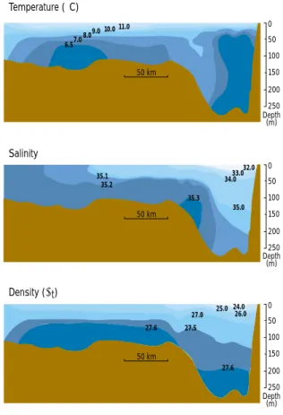
Geography, hydrography

and climate

2

GEOGRAPHY

2.1

Introduction

This chapter defines the principal geographical characteristics of the Greater North Sea. Its aim is to set the scene for the more detailed descriptions of the physical, chemical, and biological characteristics of the area and the impact man’s activities have had, and are having, upon them. For various reasons, certain areas (here called ‘focus areas’) have been given special attention.

2.2

Definition of the region

The Greater North Sea, as defined in chapter one, is situated on the continental shelf of north-west Europe. It opens into the Atlantic Ocean to the north and, via the Channel to the south-west, and into the Baltic Sea to the east, and is divided into a number of loosely defined areas. The open North Sea is often divided into the relatively shallow southern North Sea (including e.g. the Southern Bight and the German Bight), the central North Sea, the northern North Sea, the Norwegian Trench and the Skagerrak. The shallow Kattegat is seen as a transition zone between the Baltic and the North Sea. The Greater North Sea (including its estuaries and fjords) has a surface area of about 750 000 km2_{and a}

volume of about 94 000 km3_.

2.3

Bottom topography

The bottom topography is important in relation to its effect on water circulation and vertical mixing. Flows tend to be concentrated in areas where slopes are steepest, with the current flowing along the contours. The depth of the North Sea (Figure 2.1)increases towards the Atlantic Ocean to about 200 m at the edge of the continental shelf. The Norwegian Trench, which has a sill depth (saddle point) of 270 m off the west coast of Norway and a maximum depth of 700 m in the Skagerrak, plays a major role in steering large inflows of Atlantic water into the North Sea.

The Channel is relatively shallow, and from a depth of about 30 m in the Strait of Dover deepens gradually to about 100 m in the west. Seabed topography shows evidence of river valley systems that were carved into the seabed during glacial periods when the sea level was lower.

1 2

3 4 5 6 7 8 9 10

11

12 13 14 15 16 17

18 19 20

21

22

23 24 25

1. Skagerrak 2. Norwegian Trench 3. Inner Oslofjord 4. Sandefjord 5. Drammensfjord 6. Grenlandsfjord 7. Kristiansandsfjord 8. Saudafjord 9. Bergensfjord 10. Sørfjord/Hardangerfjord 11. Kattegat

12. Elbe 13. Weser 14. Jade 15. Wadden Sea 16. Oyster Ground 17. Frisian Front 18. Dutch coastal zone 19. Scheldt estuary 20. Flemish Banks 21. Seine estuary 22. Rade de Brest 23. Thames estuary 24. Humber estuary 25. Firth of Forth 0

20 50

100 200

500 1000

In the area between The Netherlands and Great Britain, extending northwards from the Channel to the Frisian Front (45 m), average depths are between 20 and 30 m. On the north-west side of the Dutch part of the continental shelf lies the shallow area of the Dogger Bank where depths can be less than 20 m. This bank has a significant impact on the circulation in the southern North Sea and is an important fishing area.

Many estuaries and fjords flow into the North Sea (Figure 2.1). Fjords are often considered as a special type of estuary, some being quite deep with a shallower sill at the mouth.

2.4

Geology and sediments

The North Sea shelf area is an ancient continental drift depression with a general north-south axis. This depression is overlain by sedimentary deposits several kilometres thick originating from the surrounding land masses, and some of their strata contain large amounts of liquid and gaseous hydrocarbons, which are intensively exploited.

During the glacial era, multiple invasions of

Scandinavian and Scottish mountain glaciers spread over the North Sea causing large sea level changes and supplies of additional sediment into the North Sea basin. It also shaped the general style of the present underwater topography, for instance, elevations such as the Dogger-Fisher Bank and depressions like the Oyster Ground, the submerged part of the Elbe valley, Devil’s Hole, Fladen Ground and the Norwegian Trench.

Sea levels rose from the end of the last glaciation until about 6 000 years ago, but since that time there have been only minor variations. The resulting hydrographic circula-tion, as well as the wave and tidal regime, created the sediment dynamics and the sediment distribution pattern seen today. Mainly sand and gravel deposits occur in the shallower areas and fine-grained muddy sediments accumulate in many of the depressions (Figure 2.2).

Tidal flats like the Wadden Sea and the Wash receive their sediments directly or indirectly from rivers and from adjacent North Sea areas. The suspended particulate matter settles to form either sandy or muddy sediments according to its composition and the predominant local hydrodynamic conditions.

2.5

Description of the coastal margin

The coastlines of the Greater North Sea display a large variety of landscapes arising from differences in geology and vertical tectonic movements. The disappearance of the weight of ice after glaciation has led to the vertical uplift of northern coastlines. The coastlines of Norway and northern Scotland are mountainous with many rocky

islands, and are often dissected by deep fjords. Most of the Swedish and Norwegian mainland is sheltered from the open ocean by a ‘continuous’ archipelago.

The coasts of northern England and Scotland feature cliffs of various sizes, some with pebble beaches, but also intersected by river valleys. The east coast of England is characterised by estuaries such as those of the Humber and Thames, and by further expanses of sand and mud flats in areas such as the Wash. Along the Channel the coastline of south-east England is dominated by low cliffs and flooded river valleys. From east to west along the French coast of the Channel are maritime plains and estuaries, cliffs, and the rocky shore of Brittany.

From the Strait of Dover to the Danish west coast, sandy beaches and dunes prevail, with numerous estuaries (e.g. of the Scheldt, Rhine, Meuse, Weser and Elbe) and the tidal inlets and islands of the Wadden Sea. This area displays signs of slow subsidence over a geological time scale. In Denmark large lagoon-like areas exist behind long sandy beaches.

The natural coastline of the Southern Bight has been changed considerably by human intervention such as the development of towns and harbours, land reclamation projects, and coastal protection structures as well as important ports and industries at river mouths and estuaries.

Northern North Sea (chiefly

Fladen Ground)

NW of Dogger Bank

Oyster Ground Devils Hole

Elbe Rinne

Mud and sandy mud Sand

Coarse sand and gravel The

Wash

Figure 2.2 Sediment types. Named locations are areas of mud and sandy mud. Source: after Eisma (1981).

2.6

Estuaries, fjords and wetlands

Estuarine and wetland habitats occur at the transition between coast and the open sea. These shallow tidal areas have a naturally high level of productivity that, in some cases, is enhanced by an anthropogenic supply of nutrients carried by rivers. The richness of the benthic life supports high numbers of resident, overwintering, and migratory waterfowl. These areas are also important as nurseries for juvenile fish, and the intertidal shoals are attractive resting sites for seals.

However, these same habitats can suffer from the accumulation of contaminants due to net sedimentation of particles from upstream sources and the sea (see Chapter 4). Ecologically important estuaries and wetlands are found in the Limfjord, the Wadden Sea, the Wash, the Dutch Delta coast, and the Channel estuaries along the coasts of France and England.

The archipelago and the fjords along the Swedish coast in the Skagerrak and northern Kattegat are very sensitive to eutrophication and other effects of human activities. Water exchange with the open sea is restricted in several places by narrow straits and shallow sills in combination with weak tides. This region is also subject to considerable environ-mental pressure due to increasing recreational use. In typical Norwegian fjords with significant water exchange to the open sea, increased oxygen consumption in the 1980s, which remained high in the 1990s, seems to a large extent to be the result of increased eutrophication of the Skagerrak. (Aure et al., 1996).

2.7

Catchment area

River systems that discharge into the Greater North Sea

(Figure 2.1) have a total catchment area of about 850 000 km2_{, and the annual input of fresh water from}

these river systems is of the order of 300 km3_{(Table 2.1).}

The annual run-off, carrying anthropogenic contaminants to the sea from land based sources, is however highly variable, and this is important for the transport of contami-nants. Melt water from Norway and Sweden constitutes about one third of the total run-off. The rivers Elbe, Weser, Rhine, Meuse, Scheldt, Seine, Thames and Humber are the most important in the catchment area.

However, the dominating source of fresh water to the North Sea is the rivers discharging into the Baltic Sea. Its catchment area is about 1 650 000 km2_{. The net fresh}

water supply to the Baltic is about 470 km3_{/yr. This water}

leaves the Baltic with a salinity of about 10 and has a profound influence on the hydrography and water movements in the eastern parts of the North Sea. The inflow from the Baltic is an additional source of contami-nants and nutrients to the North Sea (HELCOM, 1996).

2.8

Focus Areas

Many areas in the Greater North Sea region may consist of a typical and valuable habitat for marine life, be under (anthropogenic) stress or be of strategic or economic importance, and as such deserve special attention. A number of such ‘focus areas’ have been defined in this report for the above mentioned reasons, or because scientific research has resulted in a relatively large amount of information and, hence, understanding of the functioning of such an area. Selected focus areas which serve as examples of a variety of typical areas in the Greater North Sea, are described in Table 2.2and shown in Figure 2.1.

Table 2.1 Mean annual river run-off to the North Sea. Source: adapted from NSTF (1993).

Area Run-off Catchment area

(km3_{/yr) (km}2₎

Norwegian North Sea coast 58 – 70 45 500

Skagerrak and Kattegat coasts 58 – 70 102 200

Danish and German coasts

(including their Wadden Sea coasts) 32 219 900

Dutch and Belgian coasts

(including Dutch Wadden Sea, Rhine, Meuse and Scheldt) 91 – 97 221 400

English and French Channel coasts

(including Seine) 9 – 37 137 000

English east coast

(including Tyne, Tees, Humber, Thames) 32 74 500

Scottish coast

(including Forth) 16 41 000

Total North Sea region 296 – 354 841 500

Table 2.2 Focus areas with their characteristics (see also Figure 2.1).

Focus areas Description of the geographic and hydrographic characteristics

Skagerrak-Norwegian Trench The deep Norwegian Trench in the northeastern North Sea ends up in the even deeper Skagerrak. Due to this topography large amounts of Atlantic water flow into the area. This, together with the general anti-clockwise circulation of the North Sea, causes most of the water in the North Sea to pass through this area. Moreover all the water from the Baltic Sea passes through it. It also receives major riverine inputs from Norway and Sweden. Increased oxygen consumption in the water and large amounts of contaminants in the sediments are issues of concern. The residence time of the Skagerrak surface water is typically about a month, while the deepest water (500 – 700 m) may be stationary for several years.

Norwegian fjords:

inner Oslofjord, Sandefjordsfjord, These fjords have in common that most of them have a significant fresh water supply in their inner part Drammensfjord, Grenlandfjord, where also industry and cities are located. Their fine sediments are significantly contaminated. They have a Kristiansandsfjord, Saudafjord, typical estuarine circulation in the upper layers. Some of the fjords (or parts of the fjords) have a relatively Bergenfjord, Sørfjorden/ shallow sill. In the often deep basins landward of the sill the water is generally stagnant for one or several Hardanger fjord years, depending mainly on the sill topography, the strength of vertical mixing, and the hydrography outside

the fjords. The residence time of the surface water depends mainly on the length of the fjord and the freshwater discharge.

Kattegat The relatively shallow Kattegat has an estuarine-like circulation. The almost fresh water from the Baltic Sea overlays the saltier water from the Skagerrak, coming from the southern North Sea. The strong salinity stratification hinders vertical wind mixing of the deeper water where frequently oxygen depletion occurs. The residence time of the surface water is just a few weeks, and of the bottom water a few months.

Elbe and Weser estuaries, The Elbe and the Weser have river mouths which discharge huge volumes of (contaminated) fresh water into Jade Bay the southeastern corner of the North Sea and into the Wadden Sea.

The Jade Bay is a Wadden Sea-like tidal inshore basin connected to the open sea by a narrow channel. All three have important shipping lanes and are thus subject to intensive dredging and deepening. The Elbe and the Weser have a strong and stable vertical salinity stratification although tidal and wave activity can be very strong. In the Jade Bay small fresh water input and very strong tidal currents suppress the development of stratification.

Wadden Sea (including Ems- Extends along the North Sea coasts of The Netherlands, Germany and Denmark, from Den Helder to the Dollard) Skallingen peninsula near Esbjerg. It is a highly dynamic area of great ecological significance. With 500 km

it is the largest unbroken stretch of mudflats in the world.

According to the delimitation of the trilateral cooperation, the Wadden Sea covers about 13 000 km2_,

including some 1 000 km2_{islands, 350 km}2_{salt marshes, 8 000 km}2_{tidal areas (sub-tidal and inter-tidal}

flats) and some 3 000 km2_{of offshore area. The border to the North Sea is approximately the 10 m isobath.}

Most parts of the Wadden Sea are sheltered by barrier islands and contain smaller or wider area of intertidal flats.

The Wadden Sea hydrology is mainly determined by the daily tides. With each high tide an average of 15 km3_{of North Sea waters enters the Wadden Sea, thereby doubling the volume from 15 km}3_{to about}

30 km3_.

With the North Sea water also nutrients and suspended particular matter reach the Wadden Sea, through the tidal inlets. In the North of Holland there is also a structural loss of sand to the Wadden Sea. There is a structural loss of sand from the offshore area to the tidal area causing erosion of the foreshore and beaches of several islands.

Oyster Ground, Frisian Front In contrast with the shallower parts of the North Sea, which are well-mixed from surface to bottom throughout the year, this part of the North Sea (45 m) becomes statically stratified in Spring, after a period of sufficient isolation and the stratification generally lasts through the Summer. In this area the water depth exceeds the sum of the depth of a wind mixed near-surface layer (10 – 15 m) and that of a tidally mixed near-bottom layer (10 – 30 m).

Dutch Coastal Zone The coastal zone along the entire western and northern half of the Netherlands can be considered as one of the most densely populated areas in Europe. The coastal zone is protected from the sea by natural sand-dunes (254 km) and sea dikes (34 km), beach flats (38 km) and 27 km of boulevard, beach walls and the like. The width of the coastal dunes varies between less than 200 m and more than 6 km.

HYDROGRAPHY

2.9

Introduction

This chapter reviews the physical processes that have a direct influence on the ecology of the Greater North Sea. Knowledge of these processes is required in order to link inputs of dissolved and particulate matter to their concen-trations and effects upon the ecosystem.

It also serves to distinguish between natural variability and man’s impact, and to predict the possible effects of climatic and other long-term changes/variability. It should be stressed that the functioning of the North Sea is highly dependent upon the variable water exchange with surrounding ocean areas. It is also worth noting that some important phenomena such as the resuspension of sediments and transport of matter from the southern North Sea towards the Skagerrak are highly driven by ‘events’, often related to extreme weather conditions.

2.10

Water mass characterisation

The water of the shallow North Sea consists of a varying mixture of North Atlantic water and freshwater run-off. The

salinity and temperature characteristics of different areas are strongly influenced by heat exchange with the atmosphere and local freshwater supply. The deeper waters of the North Sea consist of relatively pure water of Atlantic origin, but they too are partly influenced by surface heat exchange (especially winter cooling) and, in certain areas, slightly modified through mixing with less saline surface water.

Several water mass classifications exist for the North Sea, based on temperature and salinity distributions or on residual current patterns or stratification. The main water masses and their temperature and salinity ranges are summarised in Table 2.3and Figures 2.3and 2.4.

The circulation and distribution of these water masses is of the utmost importance in supporting biological productivity, transport and concentration of living (e.g. larvae) and non-living matter in the region.

2.10.1

Physical parameters:

salinity/temperature/light transmission

In coastal waters beyond estuaries and fjords, typical salinity ranges are 32 to 34.5, except in the Kattegat and parts of Skagerrak where the influence from the Baltic results in salinities in the ranges 10 – 25 and 25 – 34, respectively. In the open waters and especially in western

Dutch Coastal Zone (cont.) The upper shore face is a multi-barred system generated by normal wave action, while its lower part is dominated by storm sedimentation, down to the depth of about 16 m. At greater depths tidal currents play a significant role along with storm waves, keeping fine-grained sediment in suspension. Below the shore face in a water depth of 14 – 23 m a broad field of sand ridges, and in water depths greater than 20 m a large field of sand waves (height 2 – 10 m) is present.

Mixing of river water from Meuse and Rhine occurs only gradually and over long distances in a northward direction.

Scheldt estuary A well-mixed estuary with a yearly average upstream freshwater flow rate of 107 m3_{/sec. The total drainage}

area is 20 300 km2_{. The estuary consists of an alternation of transition zones: deep ebb and flood channels,}

large shallow water zones, tidal flats and dry shoals.

Flemish Banks A highly dynamic system of shallow, elongated sandbanks off the Belgian coast. The sediments consist of well-sorted fine to medium sands.

Seine Estuary It is a well-mixed estuary with a yearly average freshwater flow rate of 380 m2_{/sec. The total drainage area}

is 75 000 km2_{. The estuary is subject to large tidal differences (7 m). The principal physical and}

sedimentological phenomena are governed by this tidal regime. Rade de Brest This bay covers only 180 km2_{, but the catchment area covers 2800 km}2_.

UK estuaries UK estuaries vary considerably in their characteristics. This reflects the wide differences in the topography and geology of the catchment areas, in the extent of anthropogenic influence, and in the geographical features of the coastal areas. Generally freshwater flows are at the lower end of the range typical for estuaries feeding into the Greater North Sea. Conditions in UK estuaries are strongly influenced by large tidal ranges and water movements.

Oil and gas fields The oil and gas fields are located over most of the North Sea (cf. Section 3.10). Some substances discharged by the offshore oil and gas industry are typically found in the sediments of the Skagerrak and the Norwegian Trench, where these were earlier believed to deposit and accumulate very close to the

installations. During severe storms significant resuspension may occur in water depths even down to 100 m due to wave action.

parts of the North Sea, seasonal changes in sea surface salinity (around 35) are comparatively small.

Large annual changes can be seen in the regional distribution of sea surface salinity (SSS) (Figure 2.4), and long term salinity records of the North Sea (Figure 2.5b)also show significant variability. Relatively high salinities occurred in the 1920s, at the end of the 1960s, and from 1989-95, whereas salinities were very

CentralNorth Sea w

ater

SouthNorthS

ea wat

er

Conti

nental co

astalwater

Chan nel w

ater

S_c

ot_ti s_h

c_o a st_a l_w a_te

r

Baltic water

J

u

t

l

a

n

d

c

o

ast alw

ater D_ool eyCu rr

ent Atl a

nt ic wate r

N

o

r

w

e

g

i

a

n

c_o a st_al

wa_te

r

The width of arrows is indicative of the magnitude of volume transport. Red arrows indicate relatively pure Atlantic water. Atlantic water

(west) North North Sea water

Fair Isl_{e C} ur_r

en_t

Figure 2.3 Schematic diagram of general circulation in the North Sea. Source: after Turrell et al. (1992).

3° W 1° W 1° E 3° E 5° E 7° E 9° E 11° E

3° W 1° W 1° E 3° E 5° E 7° E 9° E 11° E

3° W 1° W 1° E 3° E 5° E 7° E 9° E 11° E

3° W 1° W 1° E 3° E 5° E 7° E 9° E 11° E 61° N

59° N

57° N

55° N

53° N

51° N

49° N

61° N

59° N

57° N

55° N

53° N

51° N

49° N

1993

January – March

Salinity

1989

January – March

Salinity

Figure 2.4 Surface salinity distribution for the winters of 1989 and 1993 as an example of interannual variability. Source of data: ICES. Table 2.3 Typical values for salinity and temperature of water

masses in the North Sea. Source: adapted from NSTF (1993).

Water mass Salinity Temperature (°C)

Atlantic water > 35 7 – 15

Atlantic water (deep) > 35 5.5 – 7.5

Channel water > 35 6 – 18

Baltic water 8.5 – 10 0 – 20

Northern North Sea water 34.9 – 35.3 6 – 16 Central North Sea water 34.75 – 35.0 5 – 10 Southern North Sea water 34 – 34.75 4 – 14

Scottish coastal water 33 – 34.5 5 – 15

Continental coastal water 31 – 34 0 – 20

Norwegian coastal water 32 – 34.5 3 – 18

Skagerrak water 32 – 35 3 – 17

Skagerrak coastal water 25 – 32 0 – 20

Kattegat surface water 15 – 25 0 – 20

low in the late 1970s and most of the 1980s. The high salinities are primarily caused by a combination of reduced freshwater input and vertical mixing, as well as increased influx of Atlantic water (see also section ‘Climate’).

North Sea sea surface temperatures (SST) show a strong yearly cycle, with amplitudes ranging from 8 °C in the Wadden Sea to less than 2 °C at the northern entrances (Figures 2.5a, 2.6a). The increasing amplitude towards the south-east is related to the greater proportion of low salinity coastal water and the reduced depth. The long-term annual mean

(Figure 2.6b)shows small differences in the North Sea area with a mean value of about 9.5 °C. The shape of the 11 °C isotherm indicates the inflow of warmer water from the English Channel into the North Sea. The lowest temperatures (Figure 2.6c)in the northern Atlantic inflow area have decreased in the 25 years period (from 1969 to 1993) by about 1 °C. The highest temperatures (Figure 2.6d)have increased in that area by about 1 °C, and in the northern North Sea by about 2 °C (Becker and Schulz, 1999). This increase has also been observed in the continental coastal zone. The ‘Cold Belt’ connected with the tidal mixing front off the East Frisian Islands – shown by the course of the 20 °C isotherm – is clearly

visible. In general, the North Sea SST seems to be rather stable (see section ‘Climate’). The long-term variability of the SST is closely correlated with the strength of the atmospheric circulation of the North Atlantic, the North Atlantic Oscillation (NAO).

Light transmission through the water column is mainly limited by the presence of suspended matter and plankton. The spatial and temporal variability in concen-trations of plankton and suspended matter results in high variability in light transmission. Figure 2.7illustrates the high turbidity associated with river outflow, high plankton concentrations and/or resuspension of bottom sediments. Such features are frequently observed in satellite images of ocean colour.

2.10.2

Stratification

In winter months, most areas of the North Sea outside the Norwegian Trench, the Skagerrak and the Kattegat are vertically well mixed. In late spring, as solar heat input increases, a thermocline (a pronounced vertical tempera-ture gradient) is established over large areas of the North Sea. The thermocline separates a heated and less dense surface layer from the rest of the water column where the winter temperature remains. The strength of the

1872 2

1882 1892 1902 1912 1922 1932 1942 1952 1962 1972 1982 1992 4 6 8 10 12 Year Month -2 o 2 4 6 8 10 12 14 16 18 20 ºC a

1873 1883 1893 1903 1913 1923 1933 1943 1953 1963 1973 1983 1993 Year 2 4 6 8 10 12 Month b 28 29 30 31 32 33 34 35 36 Salinity

Figure 2.5 Monthly mean sea surface (a) temperature and (b) salinity for the period 1873–1994 measured at Helgoland-Roads. Source of data: Becker et al. (1997).

2 3 4 5 6 7 7 4 (a) 10 11 (b) -1 -1 0 1 2 3 4 5 2 (c) 3 15 15 16 17 18 19 20 20 21 21 19 18 (d) Figure 2.6 The North Sea sea-surface temperature distribution in °C

(1969–93): (a) amplitude of the yearly cycle; (b) mean; (c) minima; (d) maxima. Source of data: Becker and Schulz (2000).

thermocline depends on the heat input and the turbulence generated by the tides and the wind. This is demonstrated in two temperature sections taken during summer, one 350 km long north-westward across the Dogger Bank from the island of Terschelling (Dutch Wadden Sea) (Figure 2.8)and one between Norway and Scotland, along 57° 17' N, in the northern North Sea, the latter also showing the salinity and density distribution (Figure 2.9). Figure 2.8demonstrates that the water is vertically well mixed along the continental coast, and also to a certain extent over the Dogger Bank.

The depth of the thermocline increases from May to September and differs regionally, in August/September being typically 50 m in the northern North Sea and 20 m in the western Channel. In autumn, the increasing number and severity of storms and seasonal cooling at the surface destroy the thermocline and mix the surface

and bottom layers. The shallow parts of the southern North Sea and the Channel remain well mixed throughout the year owing to strong tidal action. The Kattegat, Skagerrak, and Norwegian Trench region of the North Sea are strongly influenced by fresh water input, and, due to the low salinity in their upper layer, have a stable stratification all year round. The deep water in these areas is not mixed with the surface water. It is mainly renewed by subduction of saltier water origi-nating from other parts of the North Sea. The salinity stratification in these regions has large implications for their primary productivity. The spring bloom starts earlier here than in other areas where stratification due to the heating must precede the bloom. To some extent, the same applies to areas off the mouths of large conti-nental rivers.

2.10.3

Fronts

Fronts or frontal zones mark the boundaries between water masses and are a common feature in the North Sea (Figure 2.10). Fronts are important because they may restrict horizontal dispersion and because there is enhanced biological activity in these regions. They can 0 – 0.5

0.5 – 1 1 – 2 2 – 5 > 5 mg/l

Figure 2.7 Distribution of depth and time averaged concentration of suspended particulate matter in the southern North Sea. Source of data: projects NERC-NSP (UK, 1988–9), TUVAS (Germany, 1989–92) and KUSTOS (Germany, 1994–6).

0 10 20 30 40 50 60 70 80

325 300 275 250 225 200 175 150 125 100 75 50 25 0

depth (m) Dogger Bank 16 14 13 7 10 8 15 17 14 14 9 11 14 17 18 17

distance from the shore at Tershelling (km)

Figure 2.8 Vertical temperature section in °C north-northwest from Terschelling (The Netherlands) taken on 26 July 1989 and showing stratification. 0 50 100 150 200 250 0 50 100 150 200 250 0 50 100 150 200 250 Depth (m) Depth (m) Depth (m) 50 km 50 km 50 km

Temperature (°C)

Salinity

Density (σ_t) 6.57.0

8.09.0 10.0 11.0 32.0 34.033.0 35.0 35.1 35.2 35.3 24.0 25.0 26.0 27.0 27.6 27.6 27.5

Figure 2.9 Mean summer vertical temperature, salinity and density sections between Norway and Scotland along 57° 17’ N.

also mark areas where surface water is subducted to form deeper water. Three types of front are present in the North Sea: tidal fronts, upwelling fronts and salinity fronts.

Tidal fronts mark the offshore limit of regions where tide induced mixing is sufficient to keep the water column mixed in competition with the heating of the surface layer. These fronts develop in summer in the western and southern parts of the North Sea where tidal currents are sufficiently strong.

Upwelling fronts form along coasts in stratified areas when the wind forces the surface water away from the coast, thus allowing deep water to surface along the coast. The formation of such fronts are common in the Kattegat, Skagerrak and along the Norwegian coast.

Salinity fronts form where low salinity water meets water of a higher salinity. Prominent salinity fronts are the Belt front which separates the outflowing Baltic surface water from the Kattegat surface water, the Skagerrak front separating the Kattegat surface water from the Skagerrak surface water and the front on the offshore side of the Norwegian coastal current (Figure 2.11). Fronts can have currents, meanders and eddies associated with them.

In many near-shore regions of the North Sea, strong tidal currents are oriented parallel to the coast. In areas such as the Rhine/Meuse outflow, for example, river water spreads along the Dutch coastline. This water overlies the denser, more saline sea water, and a pattern of estuarine circulation is established perpen-dicular to the coast. The concentrations of any

contaminants contained in these riverine waters can be significantly higher close to the coast, even at some distance from the estuary concerned. Abrupt changes in topography as well as unusual weather conditions can cause currents to deviate from this longshore alignment.

2.11

Circulation and volume transport

2.11.1

Circulation

The mean currents of the North Sea form a cyclonic circu-lation (Figure 2.3). The bulk of the transport in this circulation is concentrated to the northern part of the North Sea due to major water exchange with the

Norwegian Sea. The main inflow occurs along the western slope of the Norwegian Trench. Considerable inflows also take place east of the Shetland Islands and between Shetland and the Orkney Islands. Less than 10% enters through the Channel. All of these inflows are compen-sated by an outflow mainly along the Norwegian coast.

Westerly winds enhance the cyclonic circulation whereas winds from the east weaken the circulation (Dooley and Furnes, 1981). The circulation can occasion-ally reverse into an anti cyclonic direction. Observations show that the short-term variations of the horizontal Front

Stratified water Transition zone Mixed water Thermal fronts are deduced from satellite (infared) images; transition zones are calculated from the stratification parameter.

Figure 2.10 Transition zones between mixed and stratified water in the North Sea. Source: Becker (1990).

Yellow represents Atlantic water (T>7°C), dark blue represents coastal water (T< 3 °C). Clouds appear as black areas over the ocean. White arrows represent daily mean current vectors at 25m or 50m from three moorings.

Figure 2.11 An example of circulation patterns and fronts in the northern North Sea: NOAA satellite infrared images obtained for February 1986. Source: Johannessen et al. (1989).

transport in the Norwegian Trench are of the same order of magnitude as its mean value (Furnes and Saelen, 1977). In the rest of the North Sea, however, the wind-forced variations of the horizontal transport are one order of magnitude larger than its mean.

It seems as if most of the water in the different inflows from the north-west are guided eastwards (the Dooley Current) to the Norwegian trench by the topography along the 100 m depth contour. Only a small part flows

southward along the coast of Scotland and England. To demonstrate the variability in current pattern and magnitude, mean winter circulation (January-March) at 10 m depth was modelled for a year with a typically high (1990) and a year with a typically low (1985) inflow of Atlantic Water (Figure 2.12). This clearly demonstrates the much stronger currents all over the North Sea in 1990 compared to 1985. Much of the schematic circulation pattern from Figure 2.3is also revealed in the 1990 model results. While significant inflows of Atlantic Water occurred in 1990, both from the north and through the Channel (resulting in the highest salinities ever measured (Heath

et al., 1991; Ellet and Turrell, 1992)), there was a tendency in 1985 for outflow through the Channel and relatively weak inflows to the north. These drastic differences from year to year (mainly caused by differences in atmospheric forcing) explain some of the large scale differences in the salinities shown in Figure 2.4.

A part of the northern inflow in the Norwegian Trench crosses the trench north of the sill (saddle point) off

western Norway and returns northward (Furnes et al., 1986). However, before it leaves the North Sea, most of the water probably passes through the Skagerrak – with an average cyclonic ‘counter clockwise’ circulation – before leaving along the Norwegian coast. The water in the deepest part of the Skagerrak is renewed by cascades of dense water formed during cold winters over the more shallow parts west of the trench in the northern North Sea (Ljøen and Svansson, 1972).

In recent years, concern about algal blooms as the cause of serious problems for fish farming has led to a special interest in the inflow of the nutrient-rich water from continental rivers to the Skagerrak/Kattegat. Strong inflows occur in pulses, mainly during winters with strong southerly to westerly winds.

The residual flow in the Channel is to a large extent steered by the wind and tide. On average, this flow is from south-west to north-east, feeding a relatively narrow and saline core of Atlantic water through the Strait of Dover. The mean transport eastwards into the North Sea is confirmed by the evidence seen in the dispersion of radionuclides discharged by the Cap de la Hague nuclear reprocessing plant (Figure 2.13).

2.11.2

Bottom water movement

In the tidally well-mixed waters of the western and southern regions of the North Sea, large-scale movements are generally independent of depth

1990 (10 cm/s)

1985 (10 cm/s) 62° N

12°W 8°W 4°W 0°

62° N

56° N

52° N

12°W 8°W 4°W 0°

throughout the year. Elsewhere, the movement of North Sea bottom water at great depths has a very strong seasonal signal, with large areas becoming almost motionless during the summer. These areas are usually marked by depressed oxygen levels (to a minimum of about 65% saturation) and by temperatures similar to those of the preceding winter. Such a situation is typical in large areas of the central and northern North Sea at depths greater than about 70 m; an exception to this is the areas adjacent to bottom slopes where much of the water circulation is trapped. The situation is, however, usually very temporary as convection and mixing

processes in autumn cause a rapid renewal of these deep waters. The areas permanently stratified by salinity have a generally slow bottom water exchange. In the Kattegat, the bottom water is renewed in 1 – 4 months, the longest period during summer. This slow renewal, in combination with eutrophication, frequently leads to periods of low oxygen content. The slowest movement of bottom water occurs in central parts of the Skagerrak where depths exceed 700 m. Here, waters are normally replaced at a much slower rate (every 2 – 3 years), but rapid changes can occur when bottom water cascades into the Norwegian Trench in winter (Ljøen, 1981).

2.11.3

Volume transport and water balance

Because water fluxes can rarely be directly measured, water balances for the North Sea are mainly based upon model results. Due to differences between models in assumptions and forcings, different models often give different results. However, intercomparison exercises, such as during the EU NOWESP and NOMADS projects, indicate that a few of the larger models which include the surrounding waters of the North Sea seem to give quite similar results.

A compilation of literature results for residual flow through the Strait of Dover shows a range of 0.09 – 0.15 Sverdrup (1 Sverdrup = 106_m3_{/s) for flows induced by}

wind and tide (Boon et al., 1997) (Table 2.4). A recent study of transport and long-term residual circulation in the north-west European shelf using hydrodynamic models gave values of 0.01 and 0.06 Sverdrup through the Strait of Dover from 2 different models (Smith et al., 1996). In the same study, the range for net residual outflow through the northern North Sea between the Shetland Islands and Norway (~ 61º N) was 0.39 – 0.96 Sverdrup, while the inflow between the Scottish mainland and the Shetland Islands ranged from 0.14 – 1.1 Sverdrup.

The amount of water leaving the North Sea along the Norwegian coast is estimated at 1.3 – 1.8 Sverdrup (Otto

et al., 1990). The latest model results from the years 1955–98 indicate seasonal (1st – 4th quarter) average transports of: 1.5, 0.9, 1.1 and 1.4 Sverdrup, with a maximum of about 2.5 Sverdrup during the winters of 1990, 1991 and 1994. These estimated outflows that vary seasonally are in close balance with similar estimates of all the inflows to the North Sea, including the rivers. The net seasonal average inflow through the Channel was modelled to be: 0.05, -0.01, 0.02 and 0.05 Sverdrup for the same quarterly periods (Figure 2.14). The mean transport passing through the Skagerrak, estimated from observations, is 0.5 – 1.0 Sverdrup (Rodhe, 1987; Rydberg et al., 1996), of which 50% is in the surface waters. Recent modelling exercises indicate even higher transports especially during winter.

Estimating mean water transport in the North Sea from traditional measurements is made difficult by the large variability resulting from frequent changes in atmospheric forcing and changes in water density. Climatic variability also causes very large inter-annual variations in water transport. Numerical models have been used to cope with < 1

1 – 2 2 – 4 4 –6 6 – 8 8 – 10 10 – 12 12 – 14 Transit time, months

Cap de la Hague

UK

F

Figure 2.13 Dispersion of nuclear industry wastes in the Channel and the North Sea. Transit time (derived from radionuclide concentrations) for dissolved chemicals released at Cap de la Hague. Source: Breton et al. (1992).

Table 2.4 Residual flows through the Dover Strait (in Sverdrup) from literature data. Source: Boon et al. (1997).

Tide only Tide + Average wind Remarks Source

0.115 0.155 M2 tide Prandle (1978)

0.050 0.090 Based on Cs-tracer data, wind shear stress = 0.07 Pa Prandle (1984)

0.037 0.149 Averaged wind speed is SW 8 m/s, wind shear stress = 0.13 Pa Salomon (1993a)

0.038 0.114 Averaged wind over period 1983-1991 Salomon (1993b)

this large spatial and temporal variability. Figure 2.15a shows a 44 year (1955–98) time series of modelled inflow (mainly of Atlantic Water) to the northern North Sea during winter along an east-west section between Norway and the Orkney Islands (59° 17' N). The inter-annual variability was typically between 1.7 and 2.3 Sverdrup. However, in the period 1988–95 (except 1991), inflows were signifi-cantly higher indicating quite different atmospheric conditions. The latter has also been revealed in extreme wave height measurements during this last decade. The predominant flow through the Dover Strait is from west to east, but models also indicate that during spring net flux may be close to zero.

A comparison between several models calculating flushing times of water in several subregions of the North Sea (Table 2.5)clearly demonstrates that the large scale models agree to a considerable extent, and that transport calculated from hydrographic and sporadic current obser-vations can be significantly underestimated. This is particularly the case for the central North Sea and the English coast where the ICES flushing time estimates are of the order of 10 times longer than the model results (Backhaus, 1984; Lenhart and Pohlmann, 1997).

The flushing time for the entire North Sea, including the Norwegian Trench, is estimated to be about 1 year, whereas it is only 4 months for the Norwegian Trench part (Otto et al., 1990). Recent modelling/observation studies of

137_{Cs discharges from Sellafield and atmospheric inputs}

resulting from the Chernobyl accident indicate flushing times of approximately 500 days for the North Sea.

Using 125_{Sb and} 137_{Cs as tracers, transit times from}

Cap de la Hague were estimated to be of the order of 2 – 4 months to the Strait of Dover and 6 – 8 months to the western German Bight (Figure 2.13). These transit times are short compared to the modelled flushing times in Table 2.5 and a flushing time for the whole North Sea of about one year.

Other results from simpler model experiments tend to give flushing times that are too long (or transports that are too weak). It should be noted that in some regions, the flushing times of deep water may be much longer than in near-surface water. For example, in the Skagerrak the flushing time is of the order of years for deep water and of months for surface water. This, together with the fact that large seasonal and inter-annual variations occur, indicates that such estimates of average flushing times must be used with care.

While these values may be useful for estimating average concentrations of widely dispersed material such as nutrients derived from the Atlantic, they may have little relevance for estimating peak concentrations in situations where the local circulation close to a specific contaminant

60° N

58° N

56° N

54° N

52° N

50° N

0° 5°E 10°E 15° E

0.5 0.9

1.5

0.01

0.015

0.06 Great Britain

ALL NORTH SEA RIVERS BALTIC FRESH WATER

Sweden Denmark

Norway

Figure 2.14 Major long term modelled mean (1955–98) influx and outflux volume (in Sverdrup) of the North Sea during winter.

0.30

0.20

0.10

0.00

-0.10

-0.20

56 58 60 62 64 66 68 70 72 74 76 78 80 82 84 86 88 90 92 94 96 98

4.00 3.50 3.00 2.50 2.00 1.50 1.00 0.50 0.00

56 58 60 62 64 66 68 70 72 74 76 78 80 82 84 86 88 90 92 94 96 98

Transport (Sverdrup)

a _b

monthly mean quarterly mean

Figure 2.15 Time series of modeled volume transports in the period 1955–99: (a) into the northern North Sea between Norway and Orkneys during winter (first quarter), (b) net into the North Sea through the English Channel during spring (second quarter). Source of data: Skogen and Svendsen.

source (e.g. coastal trapping) may be crucial. For short-term phenomena of the order of days, such as plankton blooms, peak concentrations may be more sensitive to vertical exchange rates and relatively independent of the horizontal circulation (Prandle, 1990).

2.11.4

Gyres/eddies

Satellite images of the sea surface temperature invariably indicate numerous vortex-like or rotary movements on a range of scales, known as gyres or eddies. Infrared satellite images in particular (Figure 2.11)show that eddies are a common feature throughout the North Sea. They are considered an important cause of the generally observed patchiness of biota and biological processes.

Eddies may be transient, generated along frontal boundaries, or stationary, generated by topographical features. Small eddies have been observed along the Flamborough Front, located off Flamborough Head on the east coast of England. A much larger topographically generated eddy may be found to the north of the Dooley Current. More transient but very energetic eddies (typically 50 km in diameter and 200 m in depth, with a maximum current speed of about 2 m/s) are frequently found along the frontal zone of the Norwegian Coastal Current (Figure 2.11). Their origin is uncertain, but they may be generated partly by topography and partly by the pulsating outflow from the Skagerrak.

2.12

Waves, tides and storm surges

2.12.1

Waves

During storms, the resuspension and vertical dispersion

of bottom sediments due to waves and currents is a process that affects most of the North Sea, except for the deepest areas of the Skagerrak and the Norwegian Trench. Understanding this process is clearly important to the development of realistic studies of the variability in contaminant concentrations and transport. It is also important to understand the processes of wave-current interactions that can produce abnormal waves, which are potentially dangerous for example, to shipping and offshore structures. In recent years, extreme-wave analysis for specific locations has also been relevant to site selection for fish farms.

Extensive measurements have been made to estimate the wave climate of the North Sea (Figure 2.16). Wave-spectrum models are operated routinely, also in conjunction with atmospheric forecasting models. Some statistical investigations show that almost all indicators representative of storminess indicate no worsening of the storm climate for the North Atlantic Ocean and the adjacent seas (von Storch, 1996). On the other hand, statistics on significant wave heights for the North-east Atlantic point to a steady increase of the order of about 2 – 3 cm/year over the last 30 years. The inconsistency of both findings may be related to the different time scales considered. Reliable wave measurements have been available only since about 1960, while the storm climate and storm surge time series are typically longer than 100 years. However, from 1960 to about 1990 the North Atlantic Oscillation has increased and so has the wind speed, as measured for example at the west coast of Norway (see Figures 2.17and 2.18). Therefore, the increase in wave heights might be a consequence of the variability in the strength of the zonal atmospheric circula-tion (Bacon and Carter, 1991; 1993). Large variacircula-tions in the mean wind direction over the North Sea have been

Table 2.5 Comparison of flushing time (days) calculations from three numerical models and derived from measurements. Source of data: Backhaus (1984), ICES (1983), Lenhart and Pohlmann (1997), Skogen et al. (1995).

Volume Model 1* Model 2 # _{Model 3} † _ICES

Subregion (km3_{) Minimum Maximum Mean Minimum Maximum (1 year, 1985) Mean}

1 6 345 21 50 38 35 48 43 142

2b 5 644 14 49 28 9 39 50 109

6 12 815 20 57 38 41 61 63 76

7a 6 190 19 68 40 32 49 89 –

7b 2 770 13 57 34 31 39 65 547

3a 3 176 18 73 36 13 41 54 –

3b 1 138 10 50 30 15 30 48 464

4 1 323 7 49 28 21 29 50 73

5a 602 10 56 33 10 § ₂₇ § ₃₂ § ₇₃ §

5b 404 2 29 11

8 – – – – – – 131 –

* Lenhart and Pohlmann (1997) #_{Backhaus (1984)}

†_{NORWECOM, Skogen et al. (1995)} §_{These models make no subdivision between subregions 5a and 5b.}

1 6 2a

2b 8

3a 7a

7b 5 10 4 9

observed (Furnes, 1992) and consequently increased fetch may also be a part of the explanation for the increased wave heights.

2.12.2

Tides

Tides in the North Sea result from the gravitational forces of the moon and sun acting on the Atlantic Ocean. The resulting oscillations propagate across the shelf edge, entering the North Sea both across the northern boundary and through the Channel. Semidiurnal tides (two per day) predominate at the latitudes concerned and are further

amplified in the North Sea by a degree of resonance with the configuration of the coasts and depth of the seabed (Vincent and Le Provost, 1988). Figure 2.19shows the amplitude and the phase of the tidal wave relative to the moon over Greenwich.

Tidal currents (Figure 2.20)are the most energetic feature in the North Sea, stirring the entire water column in most of the southern North Sea and the Channel. In addition to its predominant oscillatory nature, this cyclonic propagation of tidal energy from the ocean also forces a net residual circulation in the same direction. Although much smaller (typically 1–3 cm/s compared with the 100

100

100

100 100 75 75 75

75

75

50

75

75 100

125

125 125

150

150 150

150

175

175 200 200

200 300

300 450 250

300

225 250 275

50-year max. surge height, cm Observation site

50-year max. wave height, m Associated wave period

32

30

28 26

24

22 20

14 14

14 12 8 8

16 18

18 seconds 19 seconds 20 seconds

17 seconds

16 seconds

15 seconds

14 seconds 13 seconds

(a) (b)

Figure 2.16 Estimated 50-year extreme maxima in the North Sea: (a) surge height based on models and observations at indicated sites; (b) wave height: distribution and associated wave period. Source of data: (a) Flather (1987); (b) UK Department of Energy (1989).

6 4 2 0 -2

-6 -4

1864 1886 1908 1930 1952 1974 1996

NAO index

Figure 2.17 Time series of the winter (December to March) NAO index and 5-year running mean (thick line) in the period 1864–1997. Source: adapted from Hurrel (1995).

oscillatory tidal currents exceeding 1 m/s), the resulting net currents are persistent and account for approximately 50% of the water transport in the western North Sea.

Along the coasts, tidal currents are oriented parallel to the coast and the exchanges between coastal and offshore waters are limited. For example, riverine waters and the associated suspended particulate matter (SPM) remain close to the French coast, and move slowly northward through the Strait of Dover into the Southern Bight (Dupont et al., 1991). In certain cases the frontal region between the coastal and offshore waters is much reduced during neap tides compared to spring tides, causing significant variability in the exchange of SPM between coastal and offshore waters.

In stratified waters, the tides can generate internal waves that propagate along the interface between the two layers. These waves can have important biological effects, as a result of enhanced vertical mixing where such waves break as well as the oscillatory movement of biota into the euphotic zone via the often large vertical displacements involved.

A large tidal range is an important condition for economic tidal power generation. Tidal heights are greatly amplified in the bays along the French coast of the Channel where heights of 8 m and more are not uncommon. Estuaries in these regions are characterised by vast intertidal zones of both mud and sand, where highly mobile sediments tend to block river mouths.

Locally, extensive construction work and the

deepening of navigation channels to major ports may have a strong effect on tidal propagation. For instance, observa-tions from tide gauges in the rivers Elbe, Weser, and Ems reveal that the attenuation of tidal waves has decreased and that the travel time of tidal waves has shortened.

2.12.3

Storm surges

Storm surges can occur in the North Sea, especially along the Belgian, Dutch, German and Danish coasts

during severe storms. They sometimes cause extremely high water levels, especially when they coincide with spring tides.

Numerical models are operated routinely in conjunc-tion with atmospheric models and provide accurate predictions (± 30 cm in 90% of the cases) of flood levels. Another method relies on statistical methods and involves tracing and modelling systematic correlations within one or more series of water level measurements. These two techniques can also be used in tandem, while at the same time employing the latest data from the monitoring stations located at offshore platforms and coastal stations, in order to update the model or the predictions. This is called

0 1000 2000 3000 4000 5000

1950 1955 1960 1965 1970 1975 1980 1985 1990 1995 2000

Norway Utsira

Figure 2.18 Monthly mean cubed wind speed (in m3_{/s) from 6-hourly measurements on the Norwegian coast at Utsira (see inset).}

1m 1m 2m 2m 2m 2m 3m 3m 3m 4m 7m 7m 7m 5m 8m 4m 4m 8m 4m 4m 10m 11m 11m 7m 5m 5 m 6m 3m 3m 3m 1h 1h 12 h 11h 11h 10 h 10 h 10 h 10 h 0h 2h 3h 4h 4h 4h 5h 5h 5 h 6h 6h 6h 2h 3h 1h 7h 7h 8h 8h 9h 9h 9h

Figure 2.19 Mean spring tidal range (range lines in m) and co-tidal lines at time intervals referred to the time of the moon’s meridian passage at Greenwich.

assimilation and is used for example by the Dutch organi-sation for flood control (Philippart and Gebraad, 1997). The increase in storm surge levels is due to an increase in the annual mean sea level and not due to changes in the intensity of high-frequency atmospheric events (Annutsch and Huber, cited in von Storch, 1996). Over the last 100 years an increase in sea level of between 20 and 30 cm was observed for the Dutch coast and the German Bight respectively based on annual means.

2.13

Transport of solids

In the shallow parts of the North Sea, intensive sediment movements and associated sediment transport occur frequently, owing to wind-induced currents, tides, and/or wave action. Sea swell is an especially effective agent for resuspension. This leads to changes in seabed

topography and may also result in resuspension of conta-minants adsorbed to settled particulate matter and their transportation, and deposition elsewhere.

Due to the nature of the material and the quite different time scales involved, the transport and

sedimen-tation of suspended particulate matter and the erosion of fine sediments are difficult to distinguish and to monitor. The use of transport models is more and more common practice in the process of decision making, and in coastal zones in particular, the impact of dredging activities, land reclamation, new discharge locations, etc., is evaluated by running different scenarios of these numerical models. The development of coupled hydrodynamic and transport models has made it possible to simulate the areas of SPM deposition and fine sediment erosion in the North Sea. However, considerable effort is still required to properly validate such model results. Averaged simulations for 1979, 1985, and 1986 are shown in Figure 2.21. The deposition rates determined by this model can be compared with observed sediment accumulation data. There is satisfactory agreement between empirical and model results for the northern North Sea (Fladen Ground) and south of the Dogger Bank. However, for the

Skagerrak, the model predicts that the highest deposition rates should occur on the southern slope, whereas field measurements show that the highest rates are in the north-eastern sector (Pohlman and Puls, 1983). Table 2.6 gives details of the amounts of particulate material trans-ported annually in the North Sea. Particulate matter originating from external sources (such as adjacent seas, rivers, dumping, cliff erosion) contributes to a yearly average of about 24 x 106_{t deposited in the North Sea.}

CLIMATE

2.14

Meteorology

The North Sea is situated in temperate latitudes with a climate that is strongly influenced by the inflow of oceanic water from the Atlantic Ocean and by the large scale westerly air circulation which frequently contains low pressure systems. The extent of this influence varies over time, and the winter North Atlantic Oscillation (NAO) Index (a pressure gradient between Iceland and the Azores) governs the strength/persistence of westerly winds (Figure 2.17). The most extreme decadal change since the 1860s has occurred from about 1960 up to the present, with very weak westerly winds during the 1960s and very strong westerly winds during the early 1990s.

Although atmospheric circulation has intensified during the last decades, it is not obvious that this is the case on a time scale of 100 years. This relates to the severe weather experienced particularly during the early part of the 20th century (WASA Group, 1998), also indicated by the NAO Index (Figure 2.17).

The persistence/strength of the westerly winds has a significant effect on water transport and distribution, vertical mixing and surface heat flux. This atmospheric

0.25 0.5

0.75

1.0 1.5 2.0

3.0

2.0 3.0

3.0

3.0 5.0

4.0 5.0

3.5 3.0

5.0 4.0 5.0

3.0

Key: see numbers on the

succession in the central North Sea. Localised higher coastal values are also indicated with numbers. Figure 2.20 Contours of maximum tidal stream amplitudes in knots

circulation is also closely related to cloud cover and therefore the light conditions in the water. All this has been shown to especially strongly affect productivity and recruitment, growth and distribution of fish stocks (Svendsen et al., 1995).

Figure 2.18shows the monthly mean cubed wind speed, a measure of the energy input to the ocean from wind, from 6-hourly measurements taken since 1950 at an island west of Norway (Utsira). In addition to the well known large seasonal variability, very large variations have occurred in the wind field, and an increasing trend in the wind speed, which is in qualitative agreement with the NAO index, has been noted from the early 1960s until today (but broken by a calm period in the late 1970s). Large variations in mean wind direction over the North Sea have also been observed (Furnes, 1992). Their importance in driving the inflows to and outflows from the North Sea has been clearly demonstrated (see below and Figure 2.15).

As a result, the North Sea climate is characterised by large variations in wind direction and speed, a high level of cloud cover, and relatively high precipitation. Rainfall data (Figure 2.22)(Hardisty, 1990; Barrett et al., 1991; ICES, 1983) show precipitation ranging between 340 and 500 mm per year, and averaging 425 mm per year. High

levels of precipitation occur along the Norwegian coast (about 1 000 mm per year) as a result of wind-forced uplift of moist air against high, steep mountain ranges. There is roughly a balance between direct rainfall and evaporation.

2.15

Ocean climate variability

Only few really long temperature and salinity time series exist for the Greater North Sea. However, none of these series are without considerable gaps in observations. One of the longest series consists of the data from Helgoland in the inner German Bight. Observations began in the 1870s and have continued until the present day. Data gaps, especially between 1945 and 1960, were filled with corrected data from a nearby Light Vessel. Both time series (Figure 2.5)show a remarkable annual, inter-annual and decadal variability. The SST series show a weak positive trend which is in agreement with the global temperature increase of about 0.6 °C/100 yr. The salinity shows no significant trend over the 120 years of observa-tions, indicating a rather stable ratio between the advection of saline water from the North Atlantic into the North Sea and the continental run-off, here mainly from the Elbe and Weser drainage area.

0 – 20 20 – 60 60 – 200 200 – 600 > 600 0 – 20

20 – 60 60 – 200 200 – 600

Erosion g/m2

Deposition g/m2

Figure 2.21 Erosion and deposition of sediments in the North Sea. Computed annual erosion and deposition of fine sediments in the North Sea (average of three years: 1979, 1985, 1986).

Table 2.6 Supply, outflow and bottom deposition of suspended particulate matter in the North Sea (Eisma and Irion, 1988).

106_t/yr

Supply

North Atlantic ocean 10.4

Channel 22 – 30

Baltic 0.5

Rivers 4.8

Seafloor erosion ca. 9 – 13.5

Coastal erosion 2.2

Atmosphere 1.6

Primary production 1

Total supply ca. 51.5 – 64

Outflow ca. 11.4 – 14.3

Deposition

Estuaries 1.8

Wadden Sea and The Wash 5

Outer Silver Pit ca.1 – 4

Elbe Rinne ?

Oyster Ground ca. 2

German Bight 3 – 7.5

Kattegat 8

Skagerrak and Norwegian Trench ca. 17

Dumped on land 2.7

The main causes of long-term (season to 100 years) variability in the North Sea temperatures are fluctuations in surface heat exchange, wind field, inflow of Atlantic water, and freshwater input. Clearly, winter cooling has a strong effect on the water temperature of shallow regions of the North Sea, and in highly stratified areas of the Skagerrak and Kattegat where the brackish water freezes in cold years. Variable winter cooling may vary the minimum temperature of the deeper water of the northern North Sea by about 2 – 3 °C, which may be important for example for the Skagerrak bottom water renewal (Ljøen, 1981). The time series of temperature, salinity and oxygen at 600 m depth in the Skagerrak from 1952–99 illustrate the magnitude of these changes (Figure 2.23).

The variable heat input that occurs during summer is important in relation to the surface temperature, but it is relatively less important for deeper waters since the stability created during heating (thermocline) effectively prevents vertical heat exchange. Climatic changes in the North Sea can often be discerned in the temperature and salinity characteristics of bottom water masses (Svendsen and Magnusson, 1992).

It has been demonstrated by large amounts of hydro-graphic and meteorological data available for 1968–90 that the winter cloud cover is important in determining the heat content of the northern North Sea (Svendsen and Magnusson, 1992). The heat content is also strongly affected by large year-to-year variations in the inflow of relatively warm (during winter) Atlantic water, as was modelled for the years 1955–97 (see Figure 2.15). The influence of Atlantic water is important for general circula-tion in the northern North Sea and the Skagerrak. As Atlantic water is the main source of nutrients and the supply of plankton for the North Sea, this variable inflow from year to year, combined with a variable wind climate (causing an upward flux of nutrients) and heat content, is the main factor determining biological productivity in large areas of the North Sea. These climatic variables have been demonstrated to influence, directly or indirectly, the recruit-ment of several fish species in the North Sea (Svendsen

et al., 1995). It has also been demonstrated that the variable inflows directly affect the migration of adult fish into the northern North Sea (Iversen et al., 1998).

While the winters of 1989 and 1990 appear to have been the mildest for the North Sea in the last 50 years (perhaps even the last 130 years), 1977–9 and possibly 1942 were probably the coldest. The 1977–9 cold period was associated with very weak winds and a low influx of Atlantic water to the North Sea, and has, in turn, been associated with the well-known late 1970s salinity anomaly (Dicksonet al., 1988). This anomaly was a clear large-scale North Atlantic phenomenon that strongly affected all northern ocean areas, including their biology. Global models are now being developed with the objective of predicting ocean climate by means of sophisticated numerical simulations of circulation and heat exchange. The validity of such models will be demonstrated by the degree to which they can correctly simulate these extreme events.

Clearly, the extremely warm period in 1989–90 (remaining relatively warm up to 1995) is connected to the strong inflows of Atlantic water during the winters of this period (except 1991, Figure 2.15a). From continuous monthly mean modelled time series it has also been shown that the variability in transport has increased in the north which is in agreement with the increased strength and variability in wind speed shown in Figure 2.18.

Between the late 1930s and the mid-1980s, the general trend in the surface atmospheric temperature and the mean ocean temperature of the upper 30 m in Norwegian coastal waters was a decrease of about 2 °C. In deeper waters, no such clear trends have been observed. As a consequence of increasing concentrations of greenhouse gases in the atmosphere, radiation processes can be expected primarily to raise sea surface temperatures globally. However, the climate system, with its manifold components and positive and negative

< 200 mm

201 – 400 mm

401 – 600 mm

601 – 800 mm

801 – 1000 mm

1001 – 1500 mm

> 1500 mm

Nimbus-7 passive microwave imagery, calibrated by UK radar for 1978–87.

Temperature (

°

C)

34.8 34.9 35.0 35.1 35.2

35.3

_Salinity

4.5 5.0 5.5 6.0 6.5 7.0

7.5

_{Oxygen (mg/l)}

52 54 56 58 60 62 64 66 68 70 72 74 76 78 80 82 84 86 88 90 92 94 96 98

52 54 56 58 60 62 64 66 68 70 72 74 76 78 80 82 84 86 88 90 92 94 96 98

52 54 56 58 60 62 64 66 68 70 72 74 76 78 80 82 84 86 88 90 92 94 96 98

7.0

6.5

6.0

5.5

5.0

4.5

4.0

3.5

feedback mechanisms, cannot be predicted with certainty. As an example, the role of the oceans is, on the one hand, likely to delay overall temperature changes, but on the other, to enhance local scenarios because of possible changes in ocean circulation. It is assumed that north-western Europe will be an area of less rapid warming than more continental regions. At present, there are no strong indications of rapid warming except in the very deep waters of the Norwegian Sea due to reduced deep water formation.

The average rate of increase of Mean Sea Level (MSL) over the last century, as determined from tide gauge data, is of the order of 1 – 2 mm/yr at most stations. An example of the increased sea level from several stations in Europe is given in Figure 2.24. Weaker or even negative trends are observed in Scotland and Sweden, and larger increases have occurred around the German Bight, in the Wadden Sea and Dutch coastal zone, in south-eastern England, and at mid-Channel ports in England and France. The spatial pattern is similar to that determined from geological data averaged over several thousand years, indicating a tilting of the land masses.

The Intergovernmental Panel on Climate Change (IPCC) has reported that it is difficult to determine the possible regional effects of climate change (IPCC, 1996). However, in the period until the year 2100, their most probable estimates for the north-eastern Atlantic areas are a surface air temperature increase of about 1.5 °C, a sea level rise of about 50 cm and a general increase in storminess and rainfall. Since the 1960s the NAO has shown the largest increase since the beginning of measurements in the 1860s, and reached an all time decadal maximum around the early 1990s (Figure 2.17). However, proxy data (from the close correlation of winter tree growth with the winter NAO index) some thousand years old, indicates several occasions when similar increases have occurred, the most recent over the last 30 years. Also paleoclimatic data show that very rapid climate changes have occurred in the North Atlantic regions over time scales of 10 to 100 years. There is now considerable speculation as to whether climate changes will take place over the next few decades and, if so, in

what direction. There is as yet no real method for predicting the effects that climate change might have on the North Sea ecosystem. In order to better understand the mechanisms, it is very important, therefore, that long-term monitoring of key physical (e.g. temperature and salinity), chemical (e.g. dissolved CO₂and oxygen) and biological (e.g. plankton species) variables are continued under the auspices of the relevant intergovernmental organisations. The availability of such data will make it possible to detect trends above the noise due to the natural (short-term) variability of the ecosystem. This, in turn, will lead to more precise information on the ultimate effect of climate change on the North Sea ecosystem.

STOCKHOLM

ESBJERG

ABERDEEN

HOEK VAN HOLLAND

NEWLYN

BREST

CASCAIS

1800 1850 1900 1950 2000

50 cm

Figure 2.24 Representative long-term records of relative sea level along North-east Atlantic and Baltic Sea coastlines.